Static Electric Spring and Nonlinear Oscillations

doi:10.4236/jemaa.2010.22011 Published Online February 2010 (www.SciRP.org/journal/jemaa)

Static Electric-Spring and Nonlinear Oscillations

Haiduke Sarafian

University College, The Pennsylvania State University, York, USA. Email: [email protected]

Received October 13th_{, 2009; revised November 18}th_{, 2009; accepted November 25}th_{, 2009.}

ABSTRACT

The author designed a family of nonlinear static electric-springs. The nonlinear oscillations of a massively charged particle under the influence of one such spring are studied. The equation of motion of the spring-mass system is highly nonlinear. Utilizing Mathematica [1] the equation of motion is solved numerically. The kinematics of the particle namely, its position, velocity and acceleration as a function of time, are displayed in three separate phase diagrams. Energy of the oscillator is analyzed. The nonlinear motion of the charged particle is set into an actual three-dimensional setting and animated for a comprehensive understanding.

Keywords: Static Electric-Spring, Nonlinear Oscillator, Mathematica

1. Introduction

Analysis of the kinematics and dynamics of a mechanical spring-mass system is a classic physics problem [2]. In this analysis the spring is idealized; it is assumed the spring is mass-less and linear. The first assumption is “justified” when the mass of the object outweighs the spring. The linearity for a coiled-shaped spring for most of the time is enforced by not stretching the spring be-yond its plastic limit. Under these assumptions the equa-tion describing the moequa-tion of the object is a second order linear differential equation; it is trivially solved with analytic sinusoidal solutions. This scenario is modified slightly when a nonlinear mass-less spring is considered. For instance, some 90 years ago, Duffing [3] initiated the notion of the nonlinear vibrator. Accordingly, an equation is proposed to describe the state of one such oscillator. Duffing’s equation is given by, _{x   x x x}3_{f t( );}

where, in addition to the linear spring term, x, a cubic term, _x3_{, is used to characterize the non-linearity.}

Damping and the source of the forced oscillation terms are given by, x, and f(t), respectively. The notion of Duffing’s initiated nonlinear vibrator has found its appli-cations in a wide range of scientific fields. Reference [4] for instance has sections devoted to the description of the Duffing equation. The latter reference also contains a wealth of bibliographic listed related articles. Recently, an electronic website [5] posted an animated description of the Duffing related issues. However, neither these ref-erences nor the author’s thorough literature search could identify a source describing the oscillations of an ideal/

perfect mass-less mechanical vibrator. The article that “best” aligns with one such mechanical oscillation is a suggested experiment given in [6]. The authors of the latter reference have claimed their proposed experiment would produce data that is compatible with the descrip-tion of the Duffing equadescrip-tion. However, a careful analysis of their setup and suggested analysis reveals the mass of the elastic metal strip is ignored. This leads to expect disconnect between the data and the proposed theory.

side of it. On the other side of the ring because the field is reversed and reoriented, the particle decelerates and slides to a momentarily halt at a symmetrical opposite end. Since there is no loss of energy, continuous repeti-tion of the movement is warranted and results in steady oscillations. The electric-spring in addition to being mass- less is nonlinear as well. Therefore, without idealizing the setup we are proposing a design resulting in perfect nonlinear oscillations. As mentioned earlier, in general, the shape of the nonlinear electric field is a function of shape of the configuration of the charge distribution. Hence, by replacing the ring with different geometrical shapes such as a square, a rectangle, an ellipse, an n-tagon, and etc. one may fabricate limitless practical nonlinear electric-springs.

This article is composed of seven sections. Section 1 addresses the introduction and motivations, Section 2 outlines the objectives. Section 3 deals with the analysis. Section 4 addresses the energy issues of the oscillations, Section 5 embodies the 3D animation and the accompa-nied Mathematica code, Section 6 describes the extended design features and Section 7, the last section, shares the conclusions and closing remarks.

2. Objectives

We begin with a positively charged ring of radius R. As-suming the ring is made of a conductor; its charge distri-bution is uniform. Along the symmetry axis of the ring, the electric field, intuitively and justifiably is oriented along the axis heading outward from the center extending on both sides of the ring. The field along the axis due to the symmetry of the ring is distance dependent only. For any off-axis point the field depends on other coordinates as well. Apply the superposition principal to the electric field for a point along the symmetry axis trivially calcu-lates [7]:

3 2 2 2 ( )

( )

x E x kQ

R x 



(1)

We have assumed a right handed Cartesian coordinate system, and the ring is placed in the yz plane with the x

axis stretching from left to right. The x is the distance from the center of the ring, Q is the charge on the ring and the value of k=1/(40)9.0×109 _{in MKS units. A}

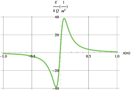
plot of E/(kQ) for a 10 cm ring size is shown in Figure 1.

EfieldRing[x_]= ₃

2 2 2 x

(R +x )

;

plotEfieldRing=Plot[EfieldRing[x]/.R10×10-2_,{x,-1,1},

PlotRangeAll,PlotStyle{Green,Thick},GridLines utomatic, AxesLabel{“x(m)”,”E/(k Q)(1/m2_)”}]

Equation (1) is an asymmetric/odd function with re-spect to x. Its plot displayed in Figure 1 shows the field for

Figure 1. Display of E/(k Q) for a ring of radius R=10 cm along the symmetry axis vs. distance x from the center of the ring

x<0 is negative. This means the vector field E on both sides of the ring orients itself away from the center of the ring. The value of the electric field and its variation vs. distance indeed may be viewed as the characteristic of the electric force that would act on a charged particle if it were placed on the symmetry axis. Now we envision placing a negatively charged particle on the axis. Under the influence of such a nonlinear force the particle attrac-tively accelerates toward the center of the ring. Accord-ing to Figure 1, the electric field and therefore the electric force are entirely nonlinear. Its strength and magnitude varies quite differently vs. the strength of an idealized linear mechanical spring. For instance, one of the pecu-liar characteristics of the field as depicted in Figure 1 is its hump; at a certain distance from the center of the ring it becomes extremum. The abscissa of the latter is a func-tion of the radius of the ring. These are:

dEfieldRing=D[EfieldRing[x],x]//Simplify;

Solve[dEfieldRing = = 0,x];{{x-(

2 R )},{x 2 R }}

decelerating it to a momentarily halt. The lack of friction preserves the energy of the particle, causing the move-ment to repeat itself endlessly. The particle therefore os-cillates; however, because of the non-linearity of the im-posed electric force the oscillation is nonlinear. The de-tailed analysis of the nonlinear oscillations along with related topics of interest follows.

3. Analysis

To form the equation describing the motion of the parti-cle we begin with Newton’s second law, F_net ma. The particle is characterized with {m,q}. At any given time the electric force is the only effective force acting on the particle, F_net F_q qE x( ) , where E(x) is subject to Equation (1). Newton’s law yields,

3

2 2 2

( )

( ) 0

( ( )) kQq x t x t

m

R x t

 



 (2)

The over-dot is defined as the derivative of the variable with respect to time, t. Equation (2) describes the motion of the particle. It is quite different from the classic equa-tion describing the linear oscillaequa-tions of a linear spring- mass system. It is a highly nonlinear differential equation. As we pointed out in the Introduction, historically, the Duffing equation is used as a pivotal equation describing the non-linear oscillations. A careful analysis of the force at hand reveals its masked correlation with the Duffing force. To unveil the correlation we expand the second term of Equation (2) about the center of the ring. Aside from the constant coefficient this gives:

Series[ ₃

2 2 2 x

(R +x )

,{x,0,8}]//PowerExpand

x/R3_{-(3 x}3_{)/(2 R}5_{)+(15 x}5_{)/(8 R}7_{)-(35 x}7_{)/(16 R}9_)+O[x]9

This shows our proposed mass-less electric-spring is an upgraded description of the Duffing force. The first two terms of the expanded function is known to describe a “soft” spring [5]; and that limits the scope of the Duffing force. Simply put, the author’s electric-spring is a superstructure version of the Duffing spring; i.e. its unexpanded function as it is used in Equation (2) embod-ies infinite odd powers of the compressed/elongated

elec-tric spring’s length; plus it describes an ideal/perfect

mass- less entity.

Now we go back to Equation (2). At the outset, it is known that the Duffing equation given in the introduction has no analytic solution. For our superstructure case too, we were not surprised failing to solve Equation (2) ana-lytically. We deploy Mathematica, but it also fails to solve symbolically. Lastly, we supply a set of practical initial conditions and by utilizing Mathematica we seek for a numeric solution. The code leading the numeric solution, along with the relevant computed kinematic quantities such as position, velocity and acceleration i.e. {x(t), v(t),a(t)}, respectively are given. The output is dis-played. For the ring and the particle we assumed {R,Q}= {10.×10-2 _{m,4.0 nC}, and {m,q}={10. mg, 3.0 nC},}

re-spectively,

values={k 9. 109_{,R10. 10}-2_{,Q4. 10}-9_{,m10. 10}-6_,

q3. 10-9_};

eqn=x”[t]+((k Q q )/m ₃

2 2 2

x[t]

(R +x[t] )

)/.values;

soleqn=NDSolve[{eqn 0,x[0]8(R/.values),x’[0]

0},x[t],{t,0,50}];

{positionx,velocityx,accx}={x[t]/.soleqn,D[x[t]/.soleqn, {t,1}],D[x[t]/.soleqn,{t,2}]};

plotx=Plot[positionx,{t,0,50},AxesLabel{“t,s”,”x,m”}, PlotStyleThick, GridLines->Automatic];plotv=Plot[ve- locityx,{t,0,50},AxesLabel{“t,s”,”v,m/s”},PlotStyle

Thick, GridLines->Automatic];

plota=Plot[accx,{t,0,50},AxesLabel{“t,s”,“a,m/s2_”},Pl

otStyleThick, GridLines->Automatic];

Show[GraphicsArray[{plotx,plotv,plota}],ImageSize

500]

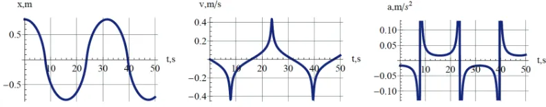
The far left graph of Figure 2 indeed confirms our speculated intuitive expected oscillations.

The particle oscillates about the origin, i.e. the center of the ring. A trained and experienced eye clearly would be able to distinguish the difference between the characteristic of this nonlinear oscillations vs. linear classic simple har-monic oscillations. From this plot alone one may deduce useful information such as period, which for the chosen utilized parameters is 32.0 s. The initial distance of the particle from the center of the ring is 8 R =0.8 m. It takes 8.0 s for the particle to make it to the center. At that

Figure 3. Plots of {x(t),v(t)}, {x(t),a(t)} and {v(t),a(t)} from left to right, respectively

instance, according to the center graph of Figure 2, the velocity of the particle is at maximum; its acceleration according to the far right graph of Figure 2 is at maxi-mum. From this instant moving forward, the particle con-tinues sliding to the left, while continually loosing speed. When the clock ticks 16.0 s its instantaneous speed plunges to zero; at that moment it reverses its motion speeds up, and accelerates toward the center of the ring.

To display the differences between the characteristics of the classic simple harmonic motion vs. our designed nonlinear oscillations, we display three phase diagrams. Utilizing Mathematica ParametricPlot we fold the time parameter and plot a set of three kinematic pairs: {x(t),v(t)}, {x(t),a(t)} and {v(t),a(t)}.

plotxv=ParametricPlot[Flatten[{positionx,velocityx}],{t, 0,50},AxesLabel{“x(m)”,“v(m/s)”},PlotStyleThick, GridLinesAutomatic,PlotRangeAll];

plotxa=ParametricPlot[Flatten[{positionx,accx}],{t,0,50} ,AxesLabel{“x(m)”,“a(m/s2_{)”},PlotStyleThick,Grid}

LinesAutomatic,PlotRangeAll];

plotva=ParametricPlot[Flatten[{velocityx,accx}],{t,0,50} ,AxesLabel{“v(m/s)”,“a(m/s2_{)”},PlotStyleThick,Gri}

dLinesAutomatic,PlotRangeAll];

Show[GraphicsArray[{plotxv,plotxa,plotva}],ImageSize

500]

As one may speculate, the shapes displayed in Figure 3 are sensitive to the chosen parameters {R,Q} and {m,q}. The interested reader may run the code for various pa-rameters.

4. Energy of the Nonlinear Oscillator

In the analysis of the classic linear harmonic oscillations one displays the interplay of the kinetic and potential energies of the oscillator vs. time, t. For a conservative setting i.e. when the friction forces are ignored, the sum of these two energies over the span of the oscillations remains constant. Utilizing the same assumption, a non- linear oscillator preserves its energy as well; however, the time dependent variation of its kinetic and the potential energies are quite different from the linear counter case. We utilize the solution of Equation (2). The potential and

kinetic energies of the oscillators are: PE=

2 _{( )} kQq R x t 2

and KE=1/2 mv(t)2_{, respectively.}

{PE,KE,totalEnergy}={

2 2

1 -kQq

R +positionx ,1/2 m

velocityx2_{,(1/2 m velocityx}2

2 2

1 -kQq

R +positionx )}

//.values;

Plot[{107 _PE,107 _KE,107 _{totalEnergy},{t,0,20},PlotStyle} {{Thick,GrayLevel[0.5]},{Thick,Black},{Thick,Dashi ng[{0.02}],GrayLevel[0.2]}},PlotRangeAll,AxesLabel

{“t,s”, “Energy,J”},GridLines Automatic]

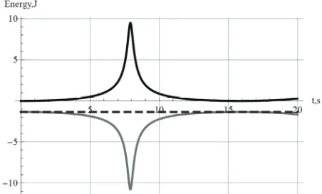
For the sake of displaying the energies with a mean-ingful scale the energies are magnified by a factor of 107_.

According to Figure 4 and as we discussed in the previ-ous section, the oscillator with an initial zero speed be-gins sliding toward the center of the ring. Since it is far-thest from the ring, its potential and kinetic energies are at minimum and zero values, respectively. These are shown by the far left tails of the curves in Figure 4. While the oscillator accelerates toward the ring, its potential energy decreases and the speeding particle gains kinetic energy. When the oscillator is at the center of the ring, its poten-tial energy is at minimum; conversely its kinetic energy is at maximum. At any given instance the sum of the values of the potential and the kinetic energies stays constant; the dashed horizontal line confirms the fact.

5. 3D Real-Life Animation and the Art Work

{{-1,1},{-1,1},{-1,1}},PlotStyle{Dashing[0.02],Thi ck}];

A sinusoidal time dependent function describes the oscil-lations of a classic linear oscillator. As an example we may envision the swinging movement of a simple pen-dulum under gravity’s pulls. How does a nonlinear oscil-lator swing? Applying the solution of Equation (2) and utilizing Mathematica’s animation feature we compose a code to bring the nonlinear oscillations to life. The ani-mation depicts a positively charged ring in red, a nega-tively charged particle in blue, and the electric field/force in green. The released particle from its initial positive position on the x-axis moves toward the ring. For the chosen ring size, the maximum value of the field/force occurs in the vicinity of its center; at

2

R

x  _{. The}

animation clearly shows the impact of the nonlinear field. i.e., when the particle makes it to the maximum field, the field jerks the particle and radically changes its move-ment.

plotlinez=ParametricPlot3D[{0,0,t},{t,-1,1},PlotRange

{{-1,1},{-1,1},{-1,1}},PlotStyle{Dashing[0.02],Thi ck}];

Show[{plot3d1,plot3d2,plotlinex,plotliney,plotlinez}]; EfieldRing3D=ParametricPlot3D[{x,0,1/40Evaluate[Ef- ieldRing[x]/.values]},{x,-1,1},PlotStyle{Green(*Gra- yLevel[0.5]*),Thick}];

Manipulate[Show[{plot3d1,plot3d2,plotlinex,plotliney, plotlinez,Graphics3D[{Blue,Sphere[{positionx[[1]]/.t  ,0,0},0.05]}],EfieldRing3D},FaceGrids{{0,0,1},{0,0, -1}},FaceGridsStyleDirective[Black,Dashed,Thickn- ess[0.003]]],{ ,0,50,0.1}] 

DynamicModule[{ =0},Show[{plot3d1,plot3d2,plotlin- ex,plotliney,plotlinez,Graphics3D[{Blue,Sphere[{positio- nx[[1]]/.t ,0,0},0.05`]}],EfieldRing3D},FaceGrids{ {0,0,1},{0,0,-1}},FaceGridsStyleDirective[Black,Das- hed,Thickness[0.003`]]]]

plot3d1=ParametricPlot3D[{0,x, _{1 x} 2 _{},{x,-1,1},Plot-}

Style{Red,Thick},PlotRange{-1,1},AxesLabel

{“x”,“y”,“z”}];

_{6. Extended Design Possibilities}

plot3d2=ParametricPlot3D[{0,x,- _{1 x} 2

},{x,-1,1},Plot-Style{Red,Thick},PlotRange{{-1,1},{-1,1},{-1,1}}, AxesLabel{“x”,“y”,“z”}];

Utilizing the concepts described in the previous section, one may readily fabricate limitless electric-springs. With-out deviating too far from what we have already described, we introduce a charged double-ring electric-spring. Show[{plot3d1,plot3d2}];

plotlinex=ParametricPlot3D[{t,0,0},{t,-1,1},PlotRange

For instance, by adjusting the values of the charge

densi-{{-1,1},{-1,1},{-1,1}},PlotStyleThick];

Figure 6. A snapshot of the motion of the negatively charged particle (the black ball), and the double-ring. The outer ring is positively charged, the inner ring is negatively charged, and each ring has its own linear charge densities. The electric field along the common ring axis is in light grey

Figure 7. Plots of {x(t),v(t)}, {x(t),a(t)} and {v(t),a(t)} are displayed in left, center and right diagrams, for the charged dou-ble-ring, respectively

ties of the rings, e.g. a positive density for the outer ring and a negative density for the inner ring, we were able to produce a double hump electric field. In Figure 6, the field is depicted in green. The positions of the humps are a func-tion of the rings’ radii. By choosing a set of appropriate radii one may set the abscissa of the humps at desired posi-tions. The field of the double-ring electric- spring shown in Figure 6 is distinctly different from the one shown in Fig-ure 1. Utilizing the former we form the equation describing the movement of a negatively charged particle. The equa-tion of moequa-tion is similar to Equaequa-tion (2). However, be-cause of the shape of the electric field the solution of the equation and therefore the description of the motion is dis-tinctly different from what we have shown in the previous section. We compose a Mathematica code and animate the motion. This is shown in Figure 6.

Applying the solution of the equation of motion we plot three phase diagrams similar to the ones displayed in Figure 3. These are shown in Figure 7.

Comparing Figure 7 with Figure 3, one clearly sees the drastic differences. The impact of the double-ring on the oscillations of the oscillator is significant. The most no-table impacts are displayed in the far left and the far right plots of Figure 7.

7. Conclusions and Remarks

has the desired characteristic. The magnitude of the field along the axis varies non-linearly with distance making the force that acts on the particle nonlinear as well. It is also shown how the design is modified. For instance the details of a coplanar charged double-ring is discussed and exhibits an interesting non-linearity behavior. A thorough literature search reveals no such practical designs have been proposed earlier. Furthermore, based on the afore-mentioned detailed discussions one realizes that the number of blue print electric-spring designs are limitless. Therefore, one may design springs to meet any practical needs. The available literature on the mechanical nonlin-ear physics phenomenon mostly is discussed from a purely theoretical view. In this article we have shown practical and applicable applications. We also would like to point out that in our study because of the slowness of the motion of the charged particle justifiably we ignored the effects of electromagnetic radiation of the oscillator.

REFERENCES

[1] S. Wolfram, “The Mathematica book,” 5th Ed., Cam-bridge University Publications, 2003.

[2] E.g. J. Marion, “Classical dynamics of particles and sys-tems,” 4th Ed., Harcourt College Publishers, 1995. [3] G. Duffing, “Erzwungene schwingungen bei

verander-licher eigen-frequenz,” F. Vieweg und Sohn, Braun-schweig, 1918.

[4] S. Strogatz, “Nonlinear dynamics and chaos,” Perseus Publishing, 1994.

[5] http://wow.scalped.orgy/article/Duffing_oscillator. [6] R. H. Ennis and G. C. McGuire, “Nonlinear physics with

Mathematica for scientists and engineers,” Published by Birdhouse, Hard Spring, Peg 605, 2001.