A Novel Spatial Clustering Algorithm Based on
Delaunay Triangulation
Xiankun Yang1,2, Weihong Cui1
1
Institute of Remote Sensing Application, Chinese Academy of Sciences, Beijing, China; 2Graduate University of Chinese Academy of Sciences, Beijing, China.
Email: [email protected].
Received August 17th, 2009; revised September 16th, 2009; accepted November 13th, 2009.
ABSTRACT
Exploratory data analysis is increasingly more necessary as larger spatial data is managed in electro-magnetic media. Spatial clustering is one of the very important spatial data mining techniques which is the discovery of interesting rela-tionships and characteristics that may exist implicitly in spatial databases. So far, a lot of spatial clustering algorithms have been proposed in many applications such as pattern recognition, data analysis, and image processing and so forth. However most of the well-known clustering algorithms have some drawbacks which will be presented later when ap-plied in large spatial databases. To overcome these limitations, in this paper we propose a robust spatial clustering algorithm named NSCABDT (Novel Spatial Clustering Algorithm Based on Delaunay Triangulation). Delaunay dia-gram is used for determining neighborhoods based on the neighborhood notion, spatial association rules and colloca-tions being defined. NSCABDT demonstrates several important advantages over the previous works. Firstly, it even discovers arbitrary shape of cluster distribution. Secondly, in order to execute NSCABDT, we do not need to know any priori nature of distribution. Third, like DBSCAN, Experiments show that NSCABDT does not require so much CPU processing time. Finally it handles efficiently outliers.
Keywords: Spatial Data Mining, Delaunay Triangulation, Spatial Clustering
1. Introduction
Data mining is a process to extract implicit, nontrivial, previously unknown and potentially useful information (such as knowledge rules, constraints, regularities) from data in databases [1,2]. The explosive growth in data and databases used in business managements, government administration, and scientific data analysis has created a need for tools that can automatically transform the proc-essed data into useful information and knowledge [3]. Spatial data mining as a subfield of data mining refers to the extraction from spatial databases of implicit knowl-edge, spatial relations or significant features or patterns that are not explicitly stored in spatial databases [4]. It is concerned with the discovery of spatial relationships and intrinsic relationships between spatial and non-spatial data. With the large amount of spatial data obtained from satellite images and geographic information systems (GIS), it is an inevitable task for humans to explore spa-tial data in detail. Spaspa-tial datasets and patterns are abun-dant in many application domains related to the Envi-ronmental Protection Agency, the National Institute of
standards and Technology, and the Department of Transportation. Challenges in spatial data mining arise from the following issues [3,5]. Firstly, classical data mining is designed to process numbers and categories. In contrast, spatial data is more complex and includes ex-tended objects such as points, lines and polygons. Sec-ondly, classical data mining works with explicit inputs, whereas, spatial predicates and attributes are often im-plicit. Finally, classical data mining treats each input independently of other inputs, while spatial patterns often exhibit continuity and high autocorrelation among nearby features.
A Novel Spatial Clustering Algorithm Based on Delaunay Triangulation 142
CLARANS. It classifies data into some groups, which together satisfy the following requirements: firstly, each group must contain at least one object; secondly, each object must belong to exactly on group. It is noticed that the second requirement can be relaxed in some fuzzy partitioning techniques. 2) Hierarchical clustering me- thods [7,8], such as DIANA [9] and BIRCH [8]. A hier-archical method creates a hierhier-archical decomposition of a given set of data objects. Hierarchical methods can be classified as agglomerative (bottom-up) or divisive (top- down), based on how the hierarchical decomposition is formed. 3) Density-based clustering methods. Their gen-eral idea is to continue growing a given cluster as long as the density (the number of objects or data points) in the “neighborhood” exceeds a threshold. Such a method is able to filter out noises (outliers) and discover clusters of arbitrary shape. Examples of density-based clustering methods include DBSCAN [10], OPTICS [11], GDB- SCAN [12] and DBRS [13]. 4) Grid-based clustering methods, such as STING [14] and WaveCluster [15]. Grid-based methods quantize the object space into a fi-nite number of cells that form a grid structure. All of the clustering operations are performed on the grid structure (i.e., on the quantized space). The main advantage of this approach is its fast processing time, which is typically independent of the number of data objects and dependent only on the number of cells in each dimension in the quantized space. 5) Model-based clustering methods. For example, COBWEB. It is clearly that no particular clus-tering method has been shown to be superior to all its competitors in all aspects. Typically, the problem is that clusters identified with one method cannot be detected by other methods [16]. This is because that many clustering methods need user-specified arguments or prior knowl-edge to produce their best results. Such information needs are supplied as density threshold values, merge/ split conditions, number of parts, prior probabilities, as-sumptions about the distribution of continuous attributes within classes, and/or kernel size for intensity testing, for example, grid size for raster-like clustering [17] and ra-dius for vector-like clustering [18]. This parame-ter-tuning is expensive and inefficient for huge data sets because it demands several trial and error steps. Clustering based on Delaunay triangulation is not a new and has been described in some papers [16, 19, 20, 21]. Kang et al [14] proposed a clustering algorithm that utilizes a Delaunay triangulation; however, there is a need in the algorithm to provide a global argument as a threshold to discriminate perimeter values or edges lengths. As a result, the algorithm is not able to detect local variations. The first non-parametric clustering algo-rithm based on the Delaunay diagram, called AMOEBA, has been proposed in Estivill-Castro and Lee [16]. It overcomes some of the problems of the static approaches that required a distance threshold to be specified, but still
fails to find relatively sparse clusters in certain situations. An upgraded version of AMOEBA, called AUTO-CLUST, has been proposed by the same authors in Estiv-ill-Castro and Lee [21].
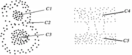
But these methods also have some drawbacks. For example, if two clusters are mixed or connected by bridges, this methods described above cannot detect all the two clusters as shown in Figure 1. In this paper we propose a robust spatial clustering algorithm named NSCABDT (Novel Spatial Clustering Algorithm Based on Delaunay Triangulation). NSCABDT uses the Delau-nay triangulation as analysis source, because DelauDelau-nay triangulation is a structure that is linear in the size of the data set and implicitly contains vast amounts of prox-imity information. That is to say, we can use the graph information of Delaunay triangulation and metric infor-mation to obtain remarkable robust clustering. In this study, we first construct a graph, and record the informa-tion of the graph as presented in Secinforma-tion 3. In the graph, vertices represent data points and edges connect pairs of points to model spatial proximity or interactions and all clustering operations are performed on the graph infor-mation.
The remainder of the paper is organized as follows: In Section 2, we will give an introduction to data preproc-essing for NSCABDT. And Section 3 presents the NSCABDT algorithm. Section 4 reports the experimental evaluation. Finally, Section 5 concludes the paper.
2. Definitions and Notions
2.1 Spatial Clustering methods
[image:2.595.311.538.572.668.2]Geographic data often show properties of spatial pendency and spatial heterogeneity [22]. Spatial de-pendency is a tendency of observations located close to one another in the geographical space to show a higher degree of similarity or dissimilarity (depending on the phenomenon under study). Closeness can be defined very generally—through distance, direction and/or topology. Spatial heterogeneity or inconsistency of the process with respect to its location is often visible, while many geographic
processes have a local character. Spatial dependency and heterogeneity can reflect the nature of the geographic process. Central to spatial data mining is clustering, which seeks to identify subsets of the data having similar characteristics. Two-Dimensional clustering is the non- trivial process of grouping geographically closer points into the cluster. Therefore, a model of spatial proximity for a discrete point-data set must pro-vide robust answers to which are the neighbors of a point
and how far the neighbors relative to the context of the entire data set
} , , {p1 pn
P
i p
P. A cluster is a group of objects, which are homogeneous among themselves. Clustering has been identified as one of the fundamental problems in the area of knowledge discovery and data mining, and it is of particular importance for spatial data sets. A dis-tinct characteristic of spatial clustering for data mining applications is the huge size of the data files involved [23]. As Tobler’s famous proposition [24] states: “Eve-rything is related to eve“Eve-rything else, but near things are more related than distant things.” Thus proximity is pretty critical to spatial analysis and in spatial settings; clustering criteria almost invariably makes use of some notions of proximity, usually based on the Euclidean metric, as it captures the essence of spatial autocorrela-tion and spatial associaautocorrela-tion [14].
2 2 2 2 2 1
1 ) ( ) ( )
( ) , ( jp ip j i j i j j x x x x x x Z X d
(1)
d(Xj, Zj)is the Euclidean metric. And
and are two dimensions
data objects.
) , , ,
(xi1 xi2 xip
)
2
) , , ,(xj1 xj2 xjp
p
(
p
We assume that is a set of
data items in the dimensional real space . A cluster is a collection of that is similar to one an-other within the same cluster and is dissimilar to the ob-jects in other clusters. A cluster of data obob-jects can be treated collectively as one group. We assume that is
a cluster of and is the collection
of , then:
} ,
, ,
{ 0 1 2 1
p p p pn
S m S } , , ,
{C1 C2 Ck
C
n
mk C S
i )
1
( k
Ci
jpiCj S
(2)
j
C Ø(
j
1
,
2
,...,
k
) (3)Ø ( ) (4)
j i C
C
i
,
j
1
,
2
,...,
j
;
i
j
If Zj is the clustering center of Cj(1 jk) , then:
k
j s C
j j j j Z p d J 1 ) ,
( (5)
where J should be minimal.
2.2 Delaunay Triangulations
In mathematics, and computational geometry, a Delau-nay triangulation for a set S of points in the plane is a triangulation D(S) such that no point in S is inside the circumcircle of any triangle in D(S). Delaunay triangula-tions maximize the minimum angle of all the angles of the triangles in the triangulation; they tend to avoid skinny triangles. The triangulation was invented by Boris Delaunay [25]. Delaunay triangulations have been widely used in a variety of applications in geographical informa-tion systems (GIS). Using Delaunay triangulainforma-tions, it is simpler to tackle the problems associated with spatial topology automated contouring, two-and-half dimen-sional (2.5-D) visualization, surface characterization and reconstructions, and site visibility analyses on terrain surfaces.
Given the set of data points in
the plane, the Voronoi region of is the locus of
points (not necessarily data points) which have as a
nearest neighbor; that is,{ .
Taken together, the n Voronoi regions of S form the Vo-ronoi diagram of S (also called the Dirichlet tessellation or the proximity map). The regions are (possibly un-bounded) convex polygons, and their interiors are dis-joint [23]. Based on Delaunay’s definition [25], the cir-cumcircle of a triangle formed by three points from the original point set is empty if it does not contain vertices other than the three that define it (other points are per-mitted only on the very perimeter, not inside).
} , , ,
{ 0 1 1
p p pn
S
S pi
i p , ( ) , ( , | 2 j i dx p
p x d i
j
)}
x
The Delaunay triangulation D(S) of S is a planar graph embedding defined as follows: the nodes of D(S) consist of the data points of S, and two nodes pi, pj are joined by an edge if the boundaries of the corresponding Voronoi regions share a line segment.
Delaunay triangulations capture in a very compact form the proximity relationships among the points of . They have many useful properties, the most relevant to our application being the following:
S
1) If pj is the nearest neighbor of pj from among the data points of S, then is an edge in D(S). That is to say, the 1-nearest-neighbor digraph is a subgraph of the Delaunay triangulation.
pi,pj
2) The number of edges in D(S) is at most 3n -6. 3) The average number of neighbors of a site in D(S) is less than six.
i
A Novel Spatial Clustering Algorithm Based on Delaunay Triangulation 144
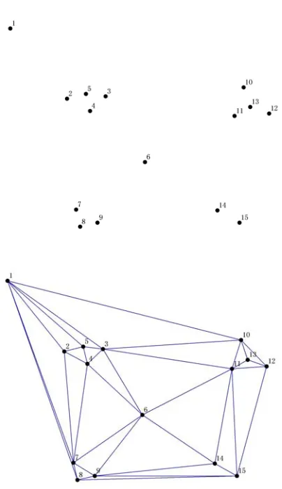
Figure 2. A data set (n=15) and its Delaunay triangulation
4) The Delaunay triangulation is the most well propor-tioned over all triangulations of S, in that the size of the minimum angle over all its triangles is the maximum possible.
5) If piand pj form a triangle in D(S), then the interior of this triangle contains no other point of S.
6) The triangulation D(S) can be robustly computed in time.
) log (n n O
7) The minimum spanning tree is a subgraph of the Delaunay triangulation, and, in fact, a single-linkage clustering (or dendrogram) can be found in
time from D(S).
) log (n n O
Figure 2 shows a set of 15 data points and its corsponding Delaunay triangulation. More information re-garding Delaunay triangulations and Voronoi diagrams can be found in other literature. From Figure 2, we can conclude that, in a proximity graph like Delaunay trian-gulation (Delaunay diagram); the points are connected by edges, if and only if they seem to be close by some proximity measure [26]. By applying to this rule, if two points are connected by a small enough Delaunay edge, the two points belong to the same cluster.
3. Initialization Using the Delaunay
Triangulations
3.1 Data Preprocessing
Given a set of data points in the
plane (as shown in Figure 2), .The triangula- tions were computed by Bowyer-Watson algorithm in time. In the creation process of Delaunay triangulation, we recorded node, edge and surface infor-mation of Delaunay triangulation for clustering later. This nodes, edges and surfaces information was stored in Oracle database. Oracle database includes numerous data structures to improve the speed of SQL queries. Taking advantage of the low cost of disk storage, Oracle in-cludes many new indexing algorithms that dramatically increase the speed with which Oracle queries are ser-viced. And, Oracle database includes so many statistical functions which include descriptive statistics, hypothesis testing, and correlations analysis, for distribution fit and so forth. The statistical functions in the database can be used in a variety of ways, for example, we can call Ora-cle’s DBMS_STAT_FUNCS functions to obtain basic cont, mean, max, min and standard deviation information of Delaunay triangulation edges. For Figure 2, we got three tables as follows:
} , , ,
{ 0 1 1
p p pn
S
15
n
) log (n n O
In the Table 1, the first column is the index of the points in S, the second column is X coordinate and the third column is Y coordinate respectively. The degree denotes the number of Delaunay edges which incident to a point. The “ClassType” column represents the category number after clustering process, and after clustering process if it is -1, we think the point is an outlier or noise.
In the Table 2, the second column is the index of the edge’s starting point, and the third column is the index of the edge’s end point. The length of edges is represented by the fourth column. In our algorithm, every edge is needed to be computed only once.
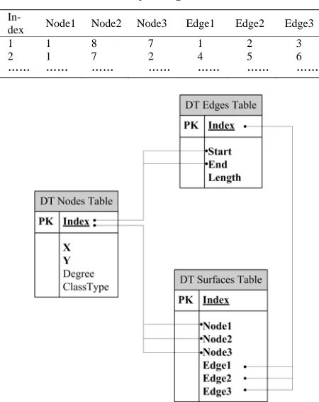
The chart illustrates the table structure and relation-ships of the three tables. The Delaunay triangulation node table contains all the spatial objects (points); the
Table 1. Delaunay triangulation nodes table
Index X Y Degree ClassType
1 3853964.924 -803305.9261 6 -1
2 3853985.696 -803331.6837 4 -1
3 3853998.714 -803330.2989 6 -1
4 3853994.005 -803335.8381 5 -1
5 3853992.066 -803329.7449 4 -1
6 3854013.393 -803354.3946 6 -1
7 3853989.297 -803371.0124 6 -1
8 3853990.128 -803377.6595 4 -1
9 3853996.221 -803375.7208 5 -1
10 3854049.121 -803327.2523 5 -1
11 3854045.52 -803337.4999 7 -1
12 3854058.538 -803336.669 4 -1
13 3854051.337 -803334.4533 3 -1
14 3854039.981 -803371.8433 4 -1
[image:4.595.311.535.553.719.2]Table 2. Delaunay triangulation edge table
Index Start End Length
1 1 8 76.03228669
2 8 7 6.69884313
3 7 1 69.50014083 4 1 7 69.50014083 5 7 2 39.49321264 6 2 1 33.08972562 7 1 2 33.08972562
8 2 5 6.65851675
9 5 1 36.11126413
10 1 5 36.11126413
[image:5.595.57.282.268.551.2]…… …… …… ……
Table 3. Delaunay triangulation surface table
In-dex Node1 Node2 Node3 Edge1 Edge2 Edge3
1 1 8 7 1 2 3
2 1 7 2 4 5 6
…… …… …… …… …… …… ……
Figure 3. Table structure and relations in the database
Delaunay triangulation edge table includes all the Delaunay edges and the relationships with the Delaunay triangula-tion node table. And the Delaunay triangulatriangula-tion surface table records all the Delaunay triangulation surfaces and the relationships with Delaunay triangulation nodes table as well as Delaunay edge table.
3.2 Some Definitions and Notions in NSCABDT Given a set of data points in the plane (as shown in Figure 2), after data preprocessing, we got the nodes, edges and surfaces information of the Delau-nay triangulation. Given a set of edges ,
for each edge
} , , ,
{ 0 1 1 p p pn
S
, {0 e
E e1,,en1}
) 1 0
( kn
ek inEis a record of Delaunay triangulation edge table. For each edge ekpi,pj,
) 1 0
( kn pi
i
p pj
is its starting point, and is its end point. Both and belong to . And denotes a set of edges which incident to .
j
p
) (pi
N i p S i p
Definition 1 (Local_Mean): We denote by mean ( ) the mean length of edges in N(pi).
) ( ) ( ) i ( _Mean Local ) i i ( d j d p
1p p i p S j e Len (6)
where denotes the degree of in graph theory; and denotes the length of the Delaunay edge
.
) (pi
d
) (ej
Len
j
e
Definition 2 (Global_Mean): We denote by mean the mean length of edges in E.
) ( ) E sum Len E ) (ej )
( _Mean S
) E ( 1 sum j Global ( sum (7)
where is the number of edges in E.
Definition 3 (Global_Sta_Dev): We denote by global standard deviation of the lengths of all edges. That is,
n e
S i
2 )) ) ( ) Len( Re Mean (p Global S Dev Sta Global n i
0( _ ( _ _ _ Local (8)Definition 4 (Relative_Mean): We let
denote the ratio of andGlobal .
That is,
) (pi Mean ) (S Mean _ lative _ ) i Mean (9) ) (S _ ) _
Relative Mean(pi)Local_Mean(pi Global Mean
Definition 5 (Positive Edge): If the length of a Delau-nay edge is less than the given criterion function , the edge is a positive edge. Positive edges and points incident to them form a new proximity graph and the newly created graph is subgraph of the Delaunay graph (Delaunay Triangulation).
) (pi
F
Definition 6 (Positive path): A path in current prox-imity graph where every edge in the path is a positive edge; and all the points connected by actives paths be-long to a cluster.
Finally, this edge analysis is captured in a criterion function . The cut-off value for edges incident in
A Novel Spatial Clustering Algorithm Based on Delaunay Triangulation 146
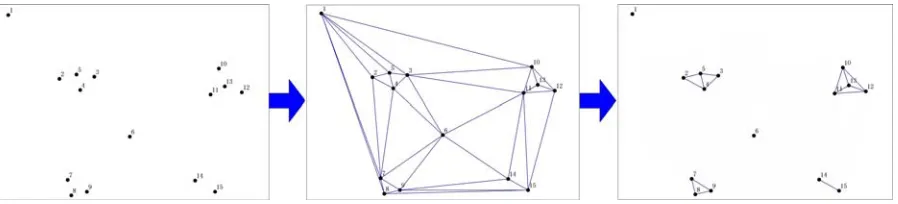
Figure 4. NSCABDT procedure
Definition 7 (Effective Region): For a point
p
in , we callS
} ,
, | | |
{x p x p S x R2
p
(11) The effective region of point p with respect to radius . As the union of the effective region of each point, we define the effective region of a random point set.
For a point set S, we call
p S
S p
(12)
The effective region of point set with respect to radius
S
.Definition 8 (γ – boundary): We define the boundary set as
)} ( {
\
,
V V V V V Dm
V (13)
where γ
>
1 is a constant and is the set of all points in the circle with the radius} | ||
{
x x Dm
. We call the γ – boundary of the point set S.
V
Definition 9 (γ – curve): The principal boundary of a random point set is the principal manifold of the point in the γ – boundary of a point set.
We also call this principal manifold extracted from point set S the γ – curve ofS.
If the edges which incident to are greater than or equal to , the edges are eliminated and the edges that are less than the criterion function survive. For each definition above, it is not necessary to iteratively calcu-late the results by programming; because we can get the results by using oracle statistical functions. For example, for Definition 1, a SQL statement can be created as fol-lows: SELECT avg(length) FROM edgetable WHERE start = , where “edgetable” is the table which restores the edges information of Delaunay triangulation.
i
p
) (pi
F
i
p
We now present the algorithm of NSCABDT:
Initialize the points of a data points set as being as-signed to no cluster; Initialize an empty data set ;
S C
1)Create Delaunay triangulation and record the in-formation of Delaunay triangulation in Oracle
da-tabase.
2)For each nodepiin Delaunay triangulation, extract
edges N(pi) incident to nodepivia SQL queries
and calculateLocal_Mean(pi)as well asF(pi). 3)For each edge
e
inN(pi), if ) ( ), the edgewill be deleted.
(e F pi
Len
4)After 3, ifd(pi)0, the node
p
iwill be deleted,otherwise, the node
p
iis added toC.5)Using the same method, iteratively calculate all the nodes which connect withpi.
6)Extract the boundary of the clusterCand eliminate the bridges.
7)If all the points have been not processed, end the process. Otherwise, initialize a new empty data setC, go to next un-processed node.
Phase 1 of NSCABDT is the construction of Delaunay triangulation. Then, recursively, all points in a connected component are reported as a cluster. Thus every edge is tested for the criterion function only once. After elimi-nating no-interesting edges and noises, only positive edges are remaining. According to the positive path, we can iteratively find all the points connected by positive paths and add the points to a cluster.
Obviously, it can be seen from the Figure 4 that it con-sists of two phases; the first phase is building Delaunay Triangulations from spatial objects. And on the second phase, we eliminate all edges in the way which we in-troduced above. And then, we got that point 1, point 6, point 14 and point 15 are outliers.
In order to eliminate the bridges between two different clusters, a detection of cluster boundary is executed; the algorithm is according to [5]. The boundary of a point set is extracted by the principal curve analysis. The principal curve analysis is a generalization of principal axis analy-sis, which is a standard method for data analysis in pat-tern recognition. For a cluster, if we can get two different boundaries, we think there are two smaller clusters in the point set, and bridges exist between the two smaller clusters. If an edge is not in the boundaries, the edge should be deleted.
different clusters is as follows:
1) For the collection of all edges E, get the median length via SQL queries. And set it as .
2) Get the effective region of random point setV . 3) Get boundaryof random point setV .
4) Get curveof random point setV.
Although, the construction of Delaunay triangulation using all points in S is a time-consuming process for a large number of points even if we use an optimal algo-rithm, we can use the information stored in the database instead of the construction of Delaunay triangulation again and we also can get the median length via SQL queries. Obviously, it is more efficient.
4. Experimental Results
We evaluate NSCABDT according the three major re-quirements for clustering algorithms on large spatial da-tabases as stated above. We compare NSCABDT with the clustering algorithm DBSCAN in terms of effectivity and efficiency. The evaluation is based on an implemen-tation of NSCABDT in .NET 2005. All the experiments were run on Windows Server 2003.
4.1 Discovery of Clusters with Arbitrary Shape
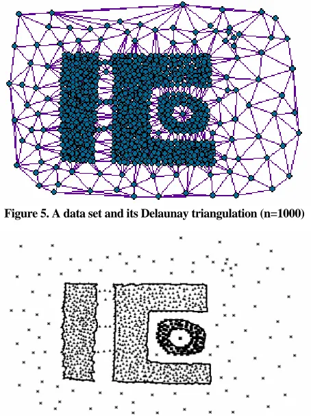
Clusters in spatial databases may be of arbitrary shape, e.g. spherical, drawn-out, linear, elongated etc. Further-more, the databases may contain noise [27]. We used visualization to evaluate the quality of the clusterings obtained by the NSCABDT. In order to create readable visualizations without using color, in these experiments we used small databases. Due to space limitation, we only present the results from one typical database which was generated as follows:
1)Draw three polygons of different shape (one of them with a hole) for three clusters.
2)Generate 500, 200 and 200 uniformly distributed points in each polygon respectively.
3)Insert 100 noise points into the database, which is depicted in Figure 5.
For NSCABDT, we set 10% noise for the sample da-tabase. NSCABDT discovers all clusters and detects the noise points from the sample database. The clustering result of NSCABDT on this database is shown in Figure 7. Different clusters are depicted using different symbols and noise is represented by crosses. This result shows that NSCABDT assigns nearly all points to the correct clusters.
4.1 Efficiency
[image:7.595.310.537.85.388.2]It has been proved that DBSCAN has better performan-cethan partitioning and hierarchical algorithms for spatial data mining, so we only compare our algorithm with DBSCAN [28]. In the following, we compare NSCA- BDT with DBSCAN with respect to efficiency on syn-
Figure 5. A data set and its Delaunay triangulation (n=1000)
Figure 6. Extract the boundary of the cluster and eliminate the bridges
Figure 7. Clustering by NSCABDT. Finally we got 3 clus-ters
[image:7.595.314.535.85.236.2]thetic databases. The run time and correct rate for NS- CABDT, DBSCAN on these test databases are listed in Table 4.
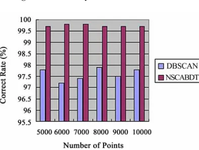
We generated some large synthetic test databases with 5000, 6000, 7000, 8000, 9000 and 10000 points to test the efficiency and scalability of DBSCAN and NSCA- BDT. We can conclude that NSCABDT is significantly slower than DBSCAN (see Figure 8), but the correct rate of NSCABDT is higher than DBSCAN (see Figure 9).
[image:7.595.318.531.424.559.2]A Novel Spatial Clustering Algorithm Based on Delaunay Triangulation 148
Table 4. Run time in seconds
Number of
Points 5000 6000 7000 8000 9000 10000
Correct rate
Run time
Correct rate
Run time
Correct rate
Run time
Correct rate
Run time
Correct rate
Run time
Correct rate
Run time
DBSCAN 97.8% 36.7 97.2% 52.8 97.4% 72.6 97.9% 93.7 97.5% 121.5 97.8% 154.6
NSCABDT 99.7% 48.2 99.8% 71.4 99.8% 93.8 99.7% 117.9 99.7% 151.3 99.7% 189.4
data, the parameters of DBSCAN is difficult to be fixed. If the parameters are not inappropriate, the correct rate will be very low. DBSCAN must continually ask for as-sistance from the user. The reliance of DBSCAN on user input can be eliminated using our approach.
5. Conclusions
The application of clustering algorithms to large spatial databases raises the following requirements [27]: 1) minimal number of input parameters, 2) discovery of clusters with arbitrary shape and 3) efficiency on large databases. The well-known clustering algorithms offer no solution to the combination of these requirements.
In this paper, we introduce the new clustering algo-rithm NSCABDT. Our notion of a cluster is based on the distance of the points of a cluster to their neighbors. The neighboring region formed in our algorithm reflects the neighbor’s distribution. Experimental results demon- strated that our clustering algorithm can provide signifi-cant improvement of accuracy of the cluster detecting, especially for objects with arbitrary and linear distribu-tion.
Figure 8. Efficiency: SCABDT VS DBSCAN
Figure 9. Correct rate: SCABDT VS DBSCAN
REFERENCES
[1] G. Piatetsky-Shapiro and W. J. Frawley. “Knowledge discovery in databases,” AAAI/MIN Press, 1999.
[2] U. Fayyad, G. Piatetsky-Shapiro, and P. Smyth. “The KDD process for extracting useful knowledge from vol-umes of data,” Communications of ACM, Vol. 39, 1996. [3] S. Shekhar, C. T. Lu, P. Zhang, and R. Liu, “Data mining
for selective visualization of large spatial datasets,” Proc-essing of 14th IEEE international conference on tools with artificial intelligence (ICTAI’02), 2002.
[4] J. Han and M. Kamber, “Data mining: Concepts and Techniques,” Academic Press, 2001.
[5] I. Atsushi and T. Ken, “Graph-based clustering of random point set,” Structural, Syntactic and Statistical Pattern Recognition, Springer Berlin, pp. 948–956, 2004.
[6] R. T. Ng and J. Han, “CLARANS: A method for cluster-ing objects for spatial data mincluster-ing,” IEEE Transactions on Knowledge and Data Engineering, Vol. 14, No. 5, pp. 1003–1016, 2002.
[7] S. Guha, R. Rastogi, and K. Shim, “CURE: An efficient clustering algorithm for large databases,” Proceedings of the 1998 ACM SIGMOD international conference on Management of data, ACM Press, pp. 73–84, 1998. [8] T. Zhang, R. Ramakrishnan, and M. Livny, “BIRCH: An
efficient data clustering method for very large databases,” Proceedings of the 1996 ACM SIGMOD international conference on Management of data, ACM Press, pp. 103–114, 1996.
[9] L. Kaufman and P. J. Rousseeuw, “Finding Groups in Data: An introduction to cluster analysis,” John Wiley & Sons, 1990.
[10] M. Ester, H. P. Kriegel, J. Sander, and X. Xu, “Density- based algorithm for discovering clusters in large spatial databases with noise,” Proceedings of the 1996 Knowl-edge Discovery and Data Mining (KDD’96) international conference, AAAI Press, pp. 226–231, 1996.
[11] M. Ankerst, M. M. Breunig, H. P. Kriegel, et al., “OP-TICS: Ordering points to identify the clustering struc-ture,” Proceedings of the International Conference on Management of Data (SIGMOD), ACM Press, pp. 49–60, 1999.
[12] J. Sander, M. Ester, H. P. Kriegel, and X. Xu, “Den-sity-Based Clustering in Spatial Databases: The algorithm GDBSCAN and its applications,” Data Mining and Knowledge Discovery, Vol. 2, No. 2, pp.169–194, 1998.
[image:8.595.74.271.557.706.2][14] R. P. Haining, “Spatial data analysis in the social and environmental sciences,” Cambridge University Press, 1990.
[15] J. Han and M. Kamber, “Data Mining: Concepts and techniques,” Second Edition, Morgan Kaufmann, 2006.
[16] V. Estivill-Castro and I. Lee, “AMOEBA: Hierarchical clustering based on spatial proximity using delaunay dia-gram,” Proceedings of the 9th international symposium on spatial data handling, pp. 7a. 26–7a. 41, 2000.
[17] E. Schikuta and M. Erhart, “The BANG-clustering sys-tem: Grid-based data analysis,” Proceedings of the 2nd international symposium IDA-97, Advances in intelligent data analysis, Springer-Verlag, pp. 513–524, 1997.
[18] S. Openshaw, “A mark 1 geographical analysis machine for the automated analysis of point data sets,” Interna-tional Journal of GIS, Vol. 1, No. 4, pp. 335–358, 1987.
[19] In-Soo Kang, Tae-wan Kim, and Ki-Joune Li, “A spatial data mining method by delaunay triangulation,” Proceed-ing of 5th ACM Workshop on Geographic Information Systems, Las Vegas, Nevada, pp. 35–39, 1997.
[20] C. Eldershaw and M. Hegland, “Cluster analysis using triangulation,” Computational Techniques and Applica-tions (CTAC97), World Scientific, Singapore, pp. 201– 208, 1997.
[21] V. Estivill-Castro and I. Lee, “AUTOCLUST: Automatic clustering via boundary extraction for mining massive point-data sets,” Proceedings of the 5th international
con-ference on geocomputation, 2000.
[22] H. J. Miller, “Geographic data mining and knowledge discovery,” Handbook of geographic information science. Malden, MA: Blackwell, pp. 149–159, 2009.
[23] V. Estivill-Castro and M. E. Houle., “Robust Distance- based clustering with applications to spatial data mining,” Algorithmica, Vol. 30, No. 2, pp. 216–242, 2001.
[24] W. R. Tobler, “A computer movie simulating urban growth in the Detroit region,” Economic Geography, Vol. 46, No. 2, pp. 234–240, 1970.
[25] B. Delaunay, “Sur la sphère vide, Izvestia Akademii Nauk SSSR, Otdelenie Matematicheskikh i Estestven- nykh Nauk,”pp. 793–800, 1934.
[26] G. Liotta, “Low degree algorithm for computing and checking gabriel graphs”, Report No. CS–96–28, De-partment of Computer Science in Brown University, Providence, 1996.
[27] X. Xu, M. Ester, H. Kriegel, and J. Sander, “A distribu-tion-based clustering algorithm for mining in large spatial databases,” Proceedings of the 14th International Con-ference on Data Engineering (ICDE’98), pp. 324–331, 1998.