Endogenous Price Flexibility and Optimal Monetary Policy

C

D

M

A

W

P

S

CASTLECLIFFE, SCHOOL OFECONOMICS& FINANCE, UNIVERSITY OFSTANDREWS, KY16 9AL

TEL: +44 (0)1334 462445 FAX: +44 (0)1334 462444 EMAIL: cdma@st-and.ac.uk

CDMA10/07

Endogenous Price Flexibility and Optimal

Monetary Policy

Ozge Senay

University of St Andrews

Alan Sutherland

†

University of St Andrews

and CEPR

FEBRUARY

2010

A

Much of the literature on optimal monetary policy uses models in which the degree of nominal price flexibility is exogenous. There are, however, good reasons to suppose that the degree of price flexibility adjusts endogenously to changes in monetary conditions. This paper extends the standard New Keynesian model to incorporate an endogenous degree of price flexibility. The model shows that endogenising the degree of price flexibility tends to shift optimal monetary policy towards complete inflation stabilisation, even when shocks take the form of cost-push disturbances. This contrasts with the standard result obtained in models with exogenous price flexibility, which show that optimal monetary policy should allow some degree of inflation volatility in order to stabilise the welfare-relevant output gap.

JEL Classification:E31, E52.

Keywords:Welfare, Endogenous Price Flexibility, Optimal Monetary Policy.

*_{School of Economics and Finance, University of St Andrews, St Andrews, KY16 9AL, UK. E-mail:} os12@st-and.ac.uk. Tel: +44 1334 462422 Fax: +44 1334 462444.

†_{School of Economics and Finance, University of St Andrews, St Andrews, KY16 9AL, UK and CEPR.}

1

Introduction

Much of the recent literature on optimal monetary policy uses models in which the degree

of nominal price flexibility is imposed exogenously (see for example Clarida, Gali and

Gertler (1999), Woodford (2003) and Benigno and Woodford (2005)). There are, however,

good theoretical and empirical reasons to suppose that the degree of price flexibility

adjusts endogenously to changes in economic conditions, including changes in monetary

policy. The ability of monetary policy to affect the real economy is closely linked to the

degree of price flexibility, so endogenous changes in price flexibility may in turn have

important effects on the design of welfare maximising monetary policy.

This paper extends the standard New Keynesian DSGE model to incorporate an

en-dogenous degree of priceflexibility and uses this model to analyse optimal monetary policy

in the face of stochastic shocks. The model is based on an adaptation of the Calvo (1983)

price setting structure. The key difference compared to the standard version of the Calvo

model is that we allow producers to choose the average frequency of price changes. We

assume that producers face costs of price adjustment which are increasing in the average

frequency of price changes and we allow producers optimally to choose the degree of price

flexibility based on the balance between the costs and benefits of price adjustment.

The model demonstrates the link between monetary policy and the equilibrium degree

of price flexibility. Monetary policy, by determining the volatility of macro variables,

affects the stochastic environment faced by producers. This has an impact on the benefits

of price flexibility for individual producers and thus affects the optimal degree of price

flexibility. For example, for a given cost of price adjustment, the greater is the volatility

of CPI inflation, the larger will be the benefits of priceflexibility for individual producers.

Producers will therefore tend to choose a greater frequency of price adjustment when the

volatility of CPI inflation is large. A monetary rule which allows volatility in CPI inflation

Having established a framework which captures the connection between monetary

policy and price flexibility, we re-examine one of the main results from the standard

literature on welfare maximising monetary policy. This result (analysed in detail by,

for instance, Woodford (2003)) is that, in the face of cost-push shocks, it is optimal

for monetary policy to allow some volatility in CPI inflation in order to stabilise the

“welfare-relevant output gap”. This result is obtained in models where the degree of

price flexibility is exogenous. How might this result be changed when the degree of price

flexibility is endogenised? Will endogenising the degree of priceflexibility make it optimal

for the monetary authority to raise or lower the volatility of inflation? On the one hand,

an increase in the volatility of inflation will tend to increase the equilibrium degree of

priceflexibility. This implies that output prices can more easily respond to shocks. But it

also reduces the ability of monetary policy to affect the real economy and thus reduce the

effectiveness of monetary policy in tackling the distortionary effects of cost-push shocks.

Our model shows that endogenising the degree of price flexibility tends to shift the

focus of optimal monetary policy towards a reduction in inflation volatility relative to

the case of exogenous price flexibility. Indeed, when the degree of price flexibility is

endogenous, it appears that optimal policy should completely stabilise CPI inflation in

the face of cost-push shocks. This is in sharp contrast to the standard result emphasised

in Woodford (2003) and Benigno and Woodford (2005). The essential point is that, lower

inflation volatility tends to reduce the equilibrium degree of price flexibility. This both

enhances the power of monetary policy and reduces the resource cost of price adjustment.

Besides demonstrating these results, this paper makes a technical modelling

contribu-tion by showing how to incorporate endogenous priceflexibility into an otherwise standard

New Keynesian model. Romer (1990), Devereux and Yetman (2002) and Yetman (2003)

have previously proposed adaptations of the Calvo model which are similar in nature

to the one described below. However, unlike Romer and Devereux and Yetman, we

widely used by the recent literature on optimal monetary policy. The optimal choice of

price flexibility in our model is based on an approximation of individual utility functions

derived directly from the microfoundations of the model. This contrasts with the Romer

and Devereux and Yetman approach, which is based on largely ad hoc macro models and

anad hoc approximation of the profit function. Note also that the main issue examined by

Romer (199) and Devereux and Yetman (2002) is the impact of a non-zero (but constant)

rate of inflation on the equilibrium degree of price flexibility. They do not consider the

impact of inflation volatility or output volatility on the equilibrium degree of price fl

exi-bility, nor do they analyse welfare maximising monetary policy in the face of stochastic

shocks.

In two further related papers Devereux and Yetman (2003, 2010) analyse exchange

rate pass-through using a version of the Calvo model which incorporates endogenous

price flexibility. These papers are particularly notable because they are amongst the

first to introduce this modification into a microfounded general equilibrium model (in

this case an open economy model). In technical terms, there are close parallels with our

modelling approach.1 _{However, Devereux and Yetman again base their analysis on an}

ad hoc approximation of the profit function. This contrasts with our approach, which is

directly based on the utility function of individual producers. Moreover, in order to solve

their model, Devereux and Yetman either assume that all shocks are i.i.d. (Devereux

and Yetman, 2003) or they make use of stochastic simulation techniques (Devereux and

Yetman, 2010). In contrast to this, we show that, for quite general cases, it is possible

to derive a closed-form representation for the relationship between producers’ utility and

the degree of price flexibility. This greatly facilitates the derivation of equilibrium in our

1_{The parallels with this paper are primarily technical. The research questions tackled by Devereux and}

Yetman (2003, 2010) are entirely focused on how priceflexibility affects exchange rate pass-through in

open economies. In contrast, we are analysing the implications of endogenous priceflexibility for optimal

model.

The model we describe clearly builds on the standard Calvo (1983) approach to price

stickiness and thus shares many of the benefits, as well as the drawbacks, of the Calvo

model. There are a number of other approaches to modelling endogenous priceflexibility,

but an important advantage of our approach is that it is based on, what has become, the

general workhorse model used throughout the monetary policy literature.

Other approaches to endogenising price flexibility include the models described by

Calmfors and Johansson (2006), Devereux (2006), Kiley (2000), Levin and Yun (2007)

and Senay and Sutherland (2006). A number of these contributions focus on the

impli-cations of endogenous price flexibility for the long run trade-off between inflation and

output, while others analyse the implication of endogenous price flexibility for the

prop-agation of monetary shocks and the causes and nature of business cycles. Only Calmfors

and Johansson (2006), Devereux (2006) and Senay and Sutherland (2006) consider the

in-teraction between endogenous priceflexibility and monetary policy choices. Calmfors and

Johansson (2006) analyse the stabilising properties of endogenising wage flexibility for a

small open economy joining a monetary union, while Devereux (2006) analyses the

impli-cations of exchange rate policy for the flexibility of prices in an open economy stochastic

general equilibrium model. In Senay and Sutherland (2006) we consider the impact of

exchange rate regime choice and price elasticity of international trade on the equilibrium

degree of price flexibility in an open economy general equilibrium model.2

2_{The degree of priceflexibility is, in a sense, also endogenous in models of state-dependent pricing. In}

these models prices may or may not adjust following a shock, depending on the size, duration and nature of

the shock, and the costs of price adjustment. This approach is considerably more difficult to implement in

a general equilibrium model suitable for analysing optimal monetary policy. Examples of state-dependent

pricing models include Devereux and Siu (2007), Dotsey, King and Wolman (1999), Dotsey and King

(2005) and Golosov and Lucas (2007). These contributions typically focus on the implications of state

dependent pricing for inflation and business cycle dynamics, as well as the propagation of monetary

This paper proceeds as follows. Section 2 describes the model. Section 3 explains

how we solve for the equilibrium level of price flexibility. Section 4 describes how the

equilibrium degree of priceflexibility is affected by different assumptions about the costs

of price adjustment and other key parameter in the model. Section 5 shows how welfare

and optimal monetary policy is affected by endogenising the degree of price flexibility.

Section 6 concludes the paper.

2

The Model

The model is a variation of the sticky-price general equilibrium structure which has become

standard in the recent literature on monetary policy. The model world consists of a single

country which is populated by farmers indexed on the unit interval. Each

yeoman-farmer consumes a basket of all goods produced in the economy and is also a monopoly

producer of a single differentiated product. In what follows, we refer to individual

yeoman-farmers as “producers” or “consumer-producers”.

Price setting follows the Calvo (1983) structure. In any given period, producer j is

allowed to change the price of good j with probability (1₋γ(j)).

The timing of events is as follows. In period0the monetary authority makes its choice

of monetary rule. Immediately following this policy decision, all producers are allowed to

make a first choice of price for trade in period 1 (and possibly beyond). Simultaneously,

all producers are also allowed the opportunity to make a once-and-for-all choice of

Calvo-price-adjustment probability (i.e. γ(j)). In each subsequent period, beginning with period

1, stochastic shocks are realised, individual producers receive their Calvo-price-adjustment

signal (which is determined by their individual choices of γ, i.e. γ(j)), those producers

which are allowed to adjust their prices do so, andfinally trade takes place.

The model economy is subject to stochastic shocks from three sources: labour supply,

2.1

Preferences

All producers have utility functions of the same form. The utility of

consumer-producer j is given by

Ut(j) =Et " _∞

X

s=t βs−t

µ C1−ρ

s (j)

1₋ρ − χKs

μ y μ s (j)

¶#

−A(γ(j)) (1)

whereC is a consumption index defined across goods, y(j)is the output of goodj andEt

is the expectations operator (conditional on time t information). K is a stochastic shock

to labour supply preferences which evolves as follows

logKt =δKlogKt−1+εK,t (2)

where 0 < δK < 1 and εK is symmetrically distributed over the interval [−ε, ε] with

E[εK] = 0 andV ar[εK] =σ2K.

The expected costs of adjusting prices are represented by the function A(γ(j)). The

form of this function is discussed in more detail below.

The consumption index C is defined as

Ct=

∙Z 1

0

ct(i)

φ−1

φ di

¸ φ φ−1

(3)

where φ >1, c(i)is consumption of goodi. The aggregate consumer price index is

Pt=

∙Z 1

0

pt(i)1−φdi ¸ 1

1−φ

(4)

The budget constraint of consumer-producer j is given by

Bt+Ct(j) =rtBt−1+pt(j)yt(j)/Pt+Rt (5)

where Bt represents holdings of risk-free real bonds at the end of periodt,rt is the gross

real rate of return on bonds and Rt is the payoffto a portfolio of state-contingent assets

The intertemporal dimension of consumption choices gives rise to the familiar

con-sumption Euler equation

C_t−ρ(j) =βrtEt £

C_t−₊₁ρ(j)¤ (6)

and individual demand for representative goodj is given by

ct(j) =Ct µ

pt(j) Pt

¶−φ

(7)

Perfect consumption risk sharing implies for alli andj

C_t−ρ(j) =C_t−ρ(i)

2.2

Government Spending Shocks

Government spending, Gt, is defined as a basket of individual goods with an aggregator

function similar to (3). Government demand for representative good j is therefore given

by

gt(j) =Gt µ

pt(j) Pt

¶−φ

(8)

Total demand for goodj is thus

yt(j) =ct(j) +gt(j) =Yt µ

pt(j) Pt

¶−φ

(9)

where aggregate output can be defined as

Yt=Ct+Gt (10)

Aggregate government spending is assumed to be a stochastic AR(1) process which evolves

as follows

Gt−G¯ =δG(Gt−1−G¯) +εG,t (11)

where G¯ is the steady state level of government spending, 0< δG<1andεG is

symmet-rically distributed over the interval [₋ε, ε] with E[εG] = 0 and V ar[εG] = σ2G. In what

2.3

Price Setting and Cost-push Shocks

In equilibrium, all producers will choose the same value of γ(j), which will be denoted

by γ. The determination of γ is discussed below. Thus, in any given period, proportion

(1₋γ) of producers are allowed to reset their prices. All producers who set their price

at time t choose the same price, denoted xt. The first-order condition for the choice of

prices implies the following

Et ( _∞

X

s=t

(βγ)s−t

" xζtYs CsρPs1−φ

− _(φφ −1)

χΛsKsYsμ Ps−φμ

#)

= 0 (12)

whereζ = 1₋φ(1₋μ)andΛis a stochastic shock to the mark-up which evolves as follows

logΛt=δΛlogΛt₋1+εΛ,t (13)

where 0 < δΛ < 1 and εΛ is symmetrically distributed over the interval [−ε, ε] with

E[εΛ] = 0 and V ar[εΛ] =σ2Λ. The first order condition can be re-written as follows

xζt = φχ

(φ₋1)

Bt Qt

(14)

where

Bt =Et ( _∞

X

s=t

(βγ)s−tΛsKsYsμP φμ s

)

Qt=Et ( _∞

X

s=t

(βγ)s−tYsCs−ρP φ−1

s )

It is possible to re-write the expression for the aggregate consumer price index as

follows

Pt= "

(1₋γ)

∞ X

s=0

γsx1t−−sφ # 1

1−φ

(15)

For the purposes of interpreting some of the results reported later, it proves useful to

consider the price that an individual producer would choose if prices could be reset every

period. This price is denotedpo

t and is given by the expression

po ζt = φχ

(φ₋1)ΛtKtY

μ−1

t P ζ tC

ρ

t (16)

2.4

Costs of Price Adjustment

Price flexibility is made endogenous in this model by allowing all producers to make a

once-and-for-all choice of the Calvo-price-adjustment probability in period zero.3 _When

making decisions with regard to price flexibility each producer acts as a Nash player.

Given that all producers are infinitesimally small, the choice of individual γ(j) is made

while assuming that the aggregate choice of γ is fixed. The equilibrium γ is assumed to

be the Nash equilibrium value (i.e. where the individual choice ofγ(j) coincides with the

aggregate γ).

Producers make their choice ofγ in order to maximise the discounted present value of

expected utility. From the point of view of the individual producer, the optimal γ is the

one which equates the marginal benefits of priceflexibility with the marginal costs of price

adjustment. The benefits of priceflexibility arise because a low value ofγ implies that the

individual price can more closely respond to shocks. The costs of price adjustment may

take the form of menu costs, information costs, decision making costs and other similar

costs. These costs of price adjustment are captured by the function A(γ(j)) in equation

(1). It is assumed that the cost of price adjustment is proportional to the expected number

of price changes per period, i.e. proportional to1₋γ(j). ThusA(γ(j))is of the following

form

A(γ(j)) = α

1₋β(1−γ(j)) (17)

where α > 0 and the factor 1/(1₋β) converts the per-period cost of price changes to

the present discounted value at time zero. It is important to note that the cost of price

flexibility is a function of the average rate of price adjustment, and is not linked to actual

3_{By restricting the choice ofγto period zero we avoid the need to track the distribution ofγ}0_{s across}

the population of producers as the economy evolves. Given that our main objective is to investigate how

the choice ofγresponds to the choice of monetary rule, and given that the choice of the monetary rule is

itself assumed to be a once-and-for-all decision, it is unlikely that much is lost by restricting the choice

price changes.

As is standard in the literature, individual producers are assumed to have access to

insurance markets which allow them to insure against the idiosyncratic income shocks

implied by the Calvo pricing structure.

2.5

Monetary Policy

Monetary policy is modelled in the form of a targeting rule. The monetary authority

is assumed to choose the monetary instrument (which is the nominal interest rate, it =

rtPt−1/Pt) in order to ensure that the following targeting relationship holds

log Pt

Pt−1

+ψlog Yt

Y∗ t

= 0 (18)

whereY∗

t is monetary authority’s target output level. We assume thatYt∗ is chosen to be the welfare maximising output level. This implies thatYt∗ is a function of labour supply,

government spending and cost-push disturbances. The determination of Y∗

t is specified in more detail below and follows the definition used in Benigno and Woodford (2005).

Thus the monetary authority follows a state-contingent inflation targeting policy where

ψ measures the degree to which inflation is allowed to vary in response to changes in the

welfare-relevant output gap. The analysis below focuses on the welfare implications of the

choice of ψ.A rule of this form is of particular interest because it is known to be optimal

in the context of a model analogous to the model outlined above but where the degree of

price flexibility is exogenously specified (see for instance Benigno and Woodford, 2005).

Note that it is not necessary to specify explicitly the form of the interest rate rule which

delivers the targeted outcome defined by (18).

3

Model Solution

It is not possible to derive an exact solution to the model described above. The model

which results when K = Λ = 1, G = ¯G and σ2

K = σ2Λ =σ2G = 0). In what follows a bar indicates the value of a variable at the non-stochastic steady state and a hat indicates the

log deviation from the non-stochastic equilibrium.4

Our objective is to solve for the Nash equilibrium value of γ. In order to do this it

is necessary to consider in detail the optimal choice of γ(j) at the level of the individual

producer. Before going into detail, however, we outline our general solution approach.

First note that, for a given value of aggregateγ it is possible to solve for the behaviour

of the aggregate economy. The behaviour of the aggregate economy is, by definition,

unaffected by the choices of an individual producer (because each

consumer-producer is assumed to be infinitesimally small). It is therefore possible to analyse the

choices of producerj while taking the behaviour of the aggregate economy as given. This

allows us to solve for the expected evolution of producer j’s output price as a function of

aggregate γ and γ(j). In turn, using the solutions for aggregate variables and producer

j’s output price, it is possible to solve for the utility of producer j for given values of γ

and γ(j).

It is thus possible to analyse producer j’s utility as a function of γ(j). In particular,

the utility maximising value of γ(j) can be identified for any given value of γ. In other

words, it is possible to plot the “best response function” of producer j to aggregate γ.

Using the best response function it is straightforward to identify Nash equilibria in the

choice ofγ. A Nash equilibrium is simply one where the utility maximising choice ofγ(j)

is equal to aggregate γ.

Below we show the detailed derivation of each stage of this solution process. We start

with the aggregate economy, then move on to producer j’s utility and prices. We are

then able to derive an explicit solution for producer j’s utility as a function of γ and

γ(j). We use a grid search technique to analyse the utility function and to plot the best

response function. This allows us to identify all possible Nash equilibria for each parameter

combination. We show the solution for aggregate prices and producer j’s prices for all

three types of shocks (labour supply, government spending and cost-push disturbances).

However, for the sake of simplicity we show the closed form solution for producer j’s

utility function for the case of cost-push shocks only. The extension to the other shocks

is straightforward.

3.1

The Aggregate Economy

For a given value of aggregateγ,the aggregate economy behaves exactly like the standard

New Keynesian model analysed by Benigno and Woodford (2005) (and many others). In

this section we summarise the equations of the aggregate model and derive first-order

accurate solutions for some of the key aggregate price variables. These solutions will then

be used in the derivation of a second-order accurate solution for the utility of producerj.

First-order approximation of equations (14) and (16) imply that the evolution of the

new contract price in period t, xˆt, is given by5

ˆ

xt= (1−βγ)(ˆpot −Pˆt) +βγEt[ˆxt+1] +O

¡ ε2¢

In turn, a first-order approximation of (15) implies that xˆt is related to consumer price

inflation as follows

ˆ

xt = γ

1₋γπt+O ¡

ε2¢

where πt = ˆPt−Pˆt−1. It is therefore possible to write a version of the New Keynesian

Phillips curve in the form

πt=

(1₋γ)(1₋βγ)

γ (ˆp o

t −Pˆt) +βEt[πt+1] +O

¡ ε2¢

Using (16) the optimal price expressed in real terms, pˆot−Pˆt,can be written as follows

ˆ

po_{t −}Pˆt=

1

ζ[ˆΛt+ ˆKt+ (μ−1) ˆYt+ρCˆt] +O ¡

ε2¢ (19)

5_{All log-deviations from the non-stochastic equilibrium are of the same order as the shocks, which (by}

assumption) are of maximum sizeε. When presenting an equation which is approximated up to ordern

which, after substituting for Yˆt usingYˆt= ˆCt+ ˆGt yields

ˆ

po_{t −}Pˆt=

1

ζ[ˆΛt+ ˆKt−ρGˆt+ (μ+ρ−1) ˆYt] +O ¡

ε2¢ (20)

It is useful to define the natural rate of output,YˆN

t ,to be theflexible price equilibrium output level. An expression forYˆN

t can be obtained from (16) by imposing the equilibrium condition pˆo

t = ˆPt, thus

ˆ

YtN =

1

(μ+ρ₋1)(−Λˆt−Kˆt+ρGˆt) +O

¡

ε2¢ (21)

Using (20) and (21) it is possible to write the real optimal price in terms of the “output

gap”

ˆ

po_{t −}Pˆt=

(μ+ρ₋1)

ζ ( ˆYt−Yˆ N t ) +O

¡

ε2¢ (22)

so the New Keynesian Phillips curve can be written in the form

πt=κ( ˆYt−YˆtN) +βEt[πt+1] +O

¡

ε2¢ (23)

where

κ= (1−γ)(1−βγ)

γ

(μ+ρ₋1)

ζ

The New Keynesian Phillips curve provides one of the key relationships which ties

down equilibrium in the macro economy. The second key relationship is provided by the

policy rule (18), which can be written in the form

πt+ψ( ˆYt−Yˆt∗) = 0 +O ¡

ε2¢ (24)

ˆ

Y∗

t is defined to be the welfare maximising output level, which following Benigno and Woodford (2005) is given by

ˆ

Y_t∗ =cΛΛˆt+cKKˆt+cGGˆt

where

cΛ = −

μΦ

cK =−

1 (μ+ρ₋1)

cG=

ρ[μ+ρ₋1₋ρΦ]

(μ+ρ₋1)[μ+ρ₋1 + (1₋ρ)Φ]

and where

Φ= 1₋ φ−1

φ

Using (22), (23) and (24) it is simple to show that the solution for pˆo

t − Pˆt can be written in the form

ˆ

po_{t −}Pˆt =pΛΛˆt+pKKˆt+pGGˆt+O ¡

ε2¢ (25)

where

pΛ =ΓΛ

1₋βδΛ

ζ , pK =ΓK

1₋βδK

ζ , pG=ΓG

1₋βδG ζ

and where

ΓΛ =

[1 +cΛ(μ+ρ−1)]ψ

κ+ψ(1₋βδΛ)

, ΓK =

[1 +cK(μ+ρ−1)]ψ κ+ψ(1₋βδK)

, ΓG =

[cG(μ+ρ−1)−ρ]ψ κ+ψ(1₋βδG)

(26)

Similarly, the solution for πt can be written in the form

πt=πΛΛˆt+πKKˆt+πGGˆt+O ¡

ε2¢ (27)

where

πΛ=ΓΛ

κ

μ+ρ₋1, πK =ΓK

κ

μ+ρ₋1, πG=ΓG

κ μ+ρ₋1

3.2

Utility of the Representative Producer

In order to derive the equilibrium value of γ it is necessary to consider the impact of the

choice of γ on the utility of a representative individual producer. The utility of producer

j at time zero (i.e. at the timeγ(j)is chosen) is given by

U0(j) =E0

∞ X

t=1

βt−1

∙

Ct1−ρ(j)

1₋ρ − χKt

μ y μ t (j)

¸

− ₁ α

The usual approach to analysing the optimal choice of a variable is to consider the

first order conditions with respect to that variable. In this case, however, the first

or-der condition of producer j’s utility maximisation problem with respect to γ(j) involves

(expectations of) derivatives which cannot be written explicitly and thus are difficult to

write even in approximated form. It is therefore easier to work directly with the utility

function of producer j, given in equation (28), and to approximate the utility function

directly. It is then possible to derive the first-order condition with respect to γ(j) using

the approximated utility function.

Before approximating the utility function there is one further complication. This is

introduced by the assumption that producers are fully insured against the consumption

risk caused by Calvo pricing uncertainty. This complication can be resolved by replacing

the true utility (28) function with the following expression

˜

U0(j) =E0

∞ X

t=1

βt−1

∙

Ct−ρ µ

yt(j)pt(j) Pt

¶

− χΛ_μtKtyμt (j) ¸

− ₁ α

−β(1−γ(j)) (29)

where the term representing the utility of consumption has been replaced by a term based

on producer j’s output, yt(j), valued using the stochastic discount factor (which is

com-mon to all households). The term representing the disutility of work effort has also been

modified to incorporate cost-push shocks (Λ). This expression has the same derivative

with respect to γ(j) as the true utility function but it pre-imposes the assumption that

all producers have the same marginal utility with respect to consumption.

Appendix A shows that a second-order approximation of (29) can be written in the

form

˜

U0(j)−U¯ =

(φ₋1)ζ

2 C¯ 1−ρ_E

0

∞ X

t=1

βt−1h₋(ˆpt(j)−Pˆt)2

+2(ˆpo_{t −}Pˆt)(ˆpt(j)−Pˆt) i

(30)

+tij− α

1₋β(1−γ(j)) +O ¡

ε3¢

where tij represents terms independent of producer j.6

We will evaluate and use (30) to analyse the optimal choice of γ(j) for producer j.

Before analysing this equation in more detail, it is useful to consider the general form of

(30) in order to understand the underlying links betweenγ(j)and producerj’s utility. The

choice of γ(j) most obviously affects utility via the costs of price adjustment. However,

γ(j)also affects utility via its impact on the evolution of producer j’s output price,pˆt(j).

Equation (30) shows that there are two routes by which the evolution of pˆt(j) affects

utility. Thefirst route arises via the termE0[(ˆpt(j)−Pˆt)2].This term effectively captures

the variance of pˆt(j) relative to the general price level. A higher variance of pˆt(j)−Pˆt

implies lower utility. Note that the variance of pˆt(j) − Pˆt depends on the difference

between the flexibility ofpˆt(j)and the flexibility ofPˆt. This is captured by the difference

between γ(j) and aggregate γ. This term is therefore likely to create a tendency for the

individual producer to prefer a value of γ(j) close to aggregate γ. The second route by

which the evolution of pˆt(j) affects utility arises via the term E0[(ˆpot −Pˆt)(ˆpt(j)−Pˆt)].

This term is effectively the covariance between the actual price charged by producerj and

the optimal price if producerj had complete freedom to choose a new price every period.

Not surprisingly, an increase in the covariance has a positive effect on utility. Also not

surprisingly, this covariance is negatively related to γ(j), i.e. the more rigid is pˆt(j) the

less correlated it can be with pˆot.7

The effect of γ(j) on utility is a combination of these three effects, i.e. it is a

com-bination of the effect on the costs of price adjustment, the variance of pˆt(j) −Pˆt and

the covariance between pˆt(j) and pˆot. An increase in γ(j) will reduce the costs of price

respect to γ(j). We are thus treating γ(j) in the same way as the parameters of the monetary policy

rule are treated in the monetary policy literature where policy rules are analysed using a second-order

approximation of aggregate utility.

7_{Note that Romer (1990) and Devereux and Yetman (2002) use an ad hoc profit function of the}

formK[ˆpt(j)−pˆot]

2

. This can be expanded to yieldK£pˆ2

t(j)−2ˆpotpˆt(j) + ˆpot2

¤

.If it is noted thatpˆo2

t is

independent of the actions of producerj this can be written asK£pˆ2

t(j)−2ˆpotpˆt(j)¤+tijwhich has the

adjustment and will thus increase utility, but it will also tend to reduce the covariance

betweenpˆt(j)andpˆot which tends to reduce utility. The effect of an increase inγ(j)on the

variance of pˆt(j)−Pˆt will depend on whetherγ(j) is greater than or less than aggregate

γ. The optimal γ(j) will obviously depend on the net outcome of the interaction of all

these three factors.

3.3

Producer

j

Prices

In order to analyse equation (30) in more detail it is necessary to derive equations which

describe the evolution of producers j’s price, i.e. pˆt(j). In particular it is necessary to

derive second-order accurate solutions for E0[(ˆpot −Pˆt)(ˆpt(j)−Pˆt)]andE0[(ˆpt(j)−Pˆt)2].

This requires first-order accurate solutions for the behaviour ofpˆt(j).

Since pˆt(j)depends onxˆt(j)(i.e. the optimal price chosen when producerj is allowed

to reset the price of good j) it is first necessary to solve for the first-order accurate

behaviour of xˆt(j). Appendix B shows that the first-order condition for producer j’s

pricing decision implies

ˆ

xt(j)−Pˆt= (1−βγ(j))(ˆpot−Pˆt) +βγ(j)Et[ˆxt+1(j)−Pˆt+1] +βγ(j)Et[πt+1] +O

¡

ε2¢ (31)

By combining this with (25) it is possible to show that

ˆ

xt(j)−Pˆt=xΛΛˆt+xKKˆt+xGGˆt+O ¡

ε2¢ (32)

where

xΛ=ΓΛ

(1₋βδΛ)(1−βγ(j))(μ+ρ−1) +κζβδΛγ(j)

(1₋βδΛγ(j))(μ+ρ−1)ζ

xK =ΓK

(1₋βδK)(1−βγ(j))(μ+ρ−1) +κζβδKγ(j)

(1₋βδKγ(j))(μ+ρ−1)ζ

xG=ΓG

(1₋βδG)(1−βγ(j))(μ+ρ−1) +κζβδGγ(j)

(1₋βδGγ(j))(μ+ρ−1)ζ

Equation (32) provides one of the required components in solving forE0[(ˆpot−Pˆt)(ˆpt(j)−

ˆ

To complete the solution forE0[(ˆpot−Pˆt)(ˆpt(j)−Pˆt)]andE0[(ˆpt(j)−Pˆt)2]it is useful

to decompose the expectations operator E0 into E0D, expectations across aggregate

dis-turbances, and EC

0, expectations across the Calvo pricing signal for producer j, where

E0[.] =E0D[E0C[.]].Since aggregate disturbances and aggregate variables are independent

from the Calvo pricing signal for producerj, we may write

E0[(ˆpot −Pˆt)(ˆpt(j)−Pˆt)] =E0D[(ˆp

o

t −Pˆt)E0C[ˆpt(j)−Pˆt]]

This makes clear that it is necessary to obtain a solution for the first-order accurate

behaviour of EC

0[ˆpt(j)−Pˆt].8 Appendix B shows that the first-order accurate behaviour of E0C[ˆpt(j)−Pˆt] is governed by the following

E0C[ˆpt(j)−Pˆt] =γ(j)E0C[ˆpt−1(j)−Pˆt−1] + (1−γ(j))(ˆxt(j)−Pˆt)−γ(j)πt+O ¡

ε2¢ (33)

This can be solved and combined with (25) and (32) to yield a second-order accurate

expression forE0[(ˆpot −Pˆt)(ˆpt(j)−Pˆt)].

In a similar way Appendix B shows that the second-order behaviour ofE0[(ˆpt(j)−Pˆt)2]

is governed by the following

E0[(ˆpt(j)−Pˆt)2] = γ(j)E0[(ˆpt−1(j)−Pˆt−1)2] +γ(j)E0[π2t]

−2γ(j)E₀D[πtE0C(ˆpt−1(j)−Pˆt−1)] (34)

+(1₋γ(j))E0[(ˆxt(j)−Pˆt)2] +O ¡

ε3¢

which can be solved in combination with (25) and (32) to yield a second-order accurate

expression forE0[(ˆpt(j)−Pˆt)2].

3.4

Closed Form Solution for Utility

Using equations (25), (27), (32), (33) and (34) we can derive a closed-form solution for

the utility of producer j. For the sake of simplicity we focus on the case where the only

8_{To be clear,E}C

0[ˆpt(j)−Pˆt]is the expected value ofpˆt(j)−Pˆtconditional on particular realised values

source of shocks is the cost-push disturbance, Λ.Extending the expression to incorporate

the other two shocks is straightforward. The resulting expression is

˜

U0(j)−U¯ = −

ζ(φ₋1) ¯C1−ρ_∆σ2 Λ

2(1₋β)(1₋βδ2)(1₋βδγ(j))(1₋βγ(j))

+tij₋ α

1₋β(1−γ(j)) +O ¡

ε3¢ (35)

where

∆ = (1₋βδΛγ(j))(1−γ(j))x2Λ+ (1 +βδΛγ(j))γ(j)π2Λ

−2βδΛγ(j)(1−γ(j))xΛπΛ−2(1−βγ(j))[(1−γ(j))xΛpΛ−γ(j)πΛpΛ]

Equation (35) shows the dependence of producer j’s utility on aggregate γ and γ(j).

This expression therefore allows us to identify producer j’s optimal choice ofγ(j) for any

given value of γ.

In principle it would be possible to analyse the optimal choice of γ(j) by examining

the derivatives of (35). The resulting expressions are however very complex. Furthermore,

because the choice ofγ(j)must lie in the[0,1]range (since it is a probability) the optimal

choice of γ(j) may be a corner solution rather than an interior solution. It is therefore

easier to analyse (35) by means of a numerical grid search technique. This is the most

reliable way to identify the global maximising value of γ(j) within the [0,1] range for

each γ in the [0,1] range. We use this grid search technique to plot the best response

function for each parameter combination. In turn, this allows us to identify all possible

Nash equilibria for each parameter combination.9

9_{Devereux and Yetman (2003) derive a closed-form solution for their model which plays a similar role}

to (35). However, their expression is only valid for the case of i.i.d. shocks. Our expression (35) is valid

for the general case of autoregressive shocks. But note that our model differs from the Devereux and

Yetman model in many respects, so our expression (35) does not encompass the equivalent expression in

Discount factor β = 0.99

Elasticity of substitution for individual goods φ= 8.00

Work effort preference parameter μ= 1.50

Elasticity of intertemporal substitution ρ= 1

Price adjustment costs α= 0.00055

Cost-push shocks δΛ = 0.9, σΛ = 0.01

Policy parameter ψ= 0.05

Table 1: Parameter Values

3.5

Calibration

We analyse the model using a wide range of parameter values, but as a benchmark we

choose the set of values shown in Table 1. Most of the values chosen are quite standard

and require no explanation. The only parameter which requires some discussion is α, i.e.

the coefficient in the function determining the costs of price adjustment. The function

A(γ(j))in principle captures a wide range of costs associated with price adjustment. Not

all these costs are directly measurable, so there is no simple empirical basis on which

to select a value for α. As a starting point, for the purposes of illustration, the value

of α is set at 0.00055 in the benchmark case. In equilibrium this implies prices are

adjusted at an average rate of once every four quarters (i.e. γ = 0.75) so aggregate price

adjustment costs are0.01375per cent of GDP in equilibrium. This total aggregate cost is

not implausibly high, given the potentially wide range of costs incorporated in A(γ(j)),

but it is acknowledged that a more satisfactory basis needs to be found for calibratingα.

In order to test the sensitivity of the main results we consider a wide range of alternative

4

The Equilibrium Degree of Price Flexibility

This section presents numerical results which illustrate the general nature and

proper-ties of equilibrium in the model described above. We also discuss the implications for

equilibriumγ of variations in the main parameters of the model.

Figure 1 illustrates some of the main features of equilibrium in the benchmark case (i.e.

the parameter set in Table 1) and a number of simple variations around that benchmark

case. Figure 1 plots the optimal value of γ(j) against values of aggregate γ. In other

words it shows the “best response function” of producer j against aggregate γ. The

benchmark case is illustrated with the plot marked with circles. This plot is nearly

horizontal, implying that the optimal value ofγ(j)is little affected by aggregateγ,and it

intersects the450just once. This point of intersection represents a single Nash equilibrium

where γ(j) =γ _≈0.75.

The position of the best response function, and its shape, are contingent on the values

of other parameters of the model. A change in the value of any parameter implies a change

in the best response function and a change in the equilibrium value of γ. Figure 1 shows

four other examples of best response function - each based on a different value of α, the

parameter which determines price adjustment costs. The general pattern that emerges

from the cases illustrated in Figure 1 is that an increase in α shifts the best response

function upwards, and thus leads to an increase in the equilibrium value of γ, while a

reduction inα shifts the best response function downwards and thus leads to a reduction

in the equilibrium value of γ. The intuition for this result is simple - an increase in the

cost of price adjustment implies that it is optimal to reduce the degree of price flexibility

(i.e. increaseγ), while a reduction in the cost of price adjustment has the opposite effect.

Figure 1 also illustrates a number of other potentially important features of the best

response function. In one of the cases shown (whereα= 0.005) the best response function

equilibrium is a corner solution at γ = 1, i.e. completely fixed prices. In other words,

when the costs of price adjustment are sufficiently high, producers optimally choose to

avoid price adjustment entirely. The next lower plot shown in Figure 1, whereα= 0.0015,

illustrates another possibility. In this case the best response function intersects the 450

line in two places. There are thus two Nash equilibria. At the other extreme, when α

is very low, it is possible to find an equilibrium where prices are completely, or almost

completelyflexible, i.e. equilibrium γ is close to zero.10

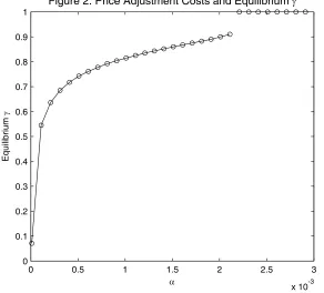
Figure 2 illustrates the relationship between equilibrium γ and the costs of price

ad-justment,α, in more detail. Thisfigure shows that equilibriumγ rises rapidly at low levels

of α,but the rate of increase then falls and equilibrium γ is relatively insensitive to αfor

values ofαgreater than 0.0005. Notice that, for values ofα greater than (approximately)

0.00022there is no Nash equilibrium within the zero-one interval. For this range ofα the

Nash equilibrium is a corner solution at γ = 1.

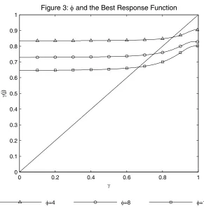
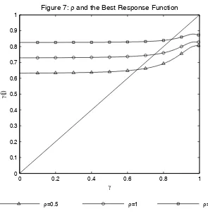
Figures 3 - 8 illustrate the effects of varying φ, the elasticity of substitution between

goods, μ, the elasticity of utility with respect to work effort, and ρ, the intertemporal

elasticity of substitution. In each case we show the impact of varying each parameter on

the best response function, and we also plot the resulting equilibrium value of γ. These

plots show that, at least for the range of parameters used here, the equilibrium γ is

relatively insensitive to variations inφ,μ andρ.

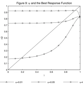
Finally, Figures 9 and 10 show the effects of varying the parameter of the monetary

policy rule,ψ. This parameter measures the degree to which policy is aimed at stabilising

inflation relative to stabilising the welfare-relevant output gap, Yˆ ₋Yˆ∗_{. The higher isψ}

the more monetary policy is aimed at stabilising the output gap, while a lower value of

10_{For some extreme parameter combinations it is possible to find knife-edge cases where the utility}

function of producerj has two peaks yielding equal utility levels. In these knife-edge cases there appears

to be no Nash equilibrium where all producers choose the sameγ(j).There may be equilibria where the

set of producers divides into two groups, each group setting a different value ofγ (corresponding to the

ψ implies that monetary policy is aimed at stabilising inflation. ψ = 0 implies complete

inflation stabilisation. Figures 9 and 10 show that the best response function of producer

j and the equilibriumγ are quite sensitive to the choice of ψ. A higher value of ψ shifts

the best response function downwards and therefore reduces the equilibrium value of γ.

In other words, the more policy focuses on stabilisation of the output gap, the greater

is equilibrium price flexibility. Conversely, the more monetary policy focuses on inflation

stabilisation, the greater will be price stickiness.

The intuition behind this result is relatively straightforward. If the monetary authority

is stabilising aggregate inflation it is by definition stabilising the desired price, pˆot. This

can be seen very clearly from equations (25), (26) and (27) which show the impact of

shocks on inflation and the desired price. These equations show that the lower is the

value of ψ, the more stable is pˆo

t. If the desired price is very stable then the incentive to incur the costs of priceflexibility are much reduced, hence producers choose a high value

of γ, i.e. more price stickiness. In the extreme case where ψ = 0 (i.e. perfect inflation

stabilisation) the equilibrium value of γ is unity, implying perfect price rigidity.

Equations (25), (26) and (27) also show that a high value of ψ (i.e. a monetary rule

which allowsfluctuations in inflation in order to achieve some stabilisation of the output

gap) will necessarily cause fluctuations in the desired price, pˆot. This raises the incentive

for producers to incur the costs of priceflexibility and therefore choose a lower value ofγ.

Figure 10 shows that, beyond a certain value of ψ (in this case approximately 0.43) the

equilibrium value of γ is zero, implying perfectlyflexible prices.

5

Welfare and Optimal Policy

We now consider the welfare implications of endogenous price flexibility. In particular

we consider the implications for the welfare maximising choice of the policy parameter,

monetary policy parameter, ψ, is set) is defined as

Ω=E0

∞ X

t=1

βt−1 ½Z 1

0

µ

Ct1−ρ(j)

1₋ρ − Kt

μ y μ t (j)

¶ dj

¾

− ₁ α

−β(1−γ) (36)

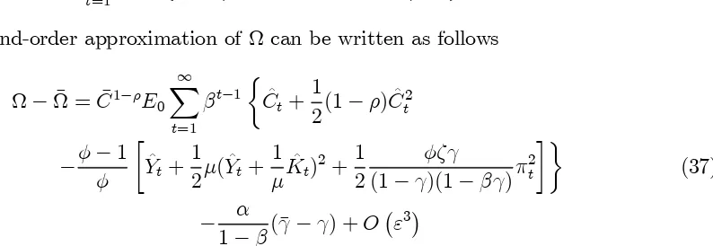
and a second-order approximation of Ω can be written as follows

Ω−Ω¯ = ¯C1−ρE0

∞ X

t=1

βt−1 ½

ˆ

Ct+

1

2(1−ρ) ˆC 2

t

−φ−_φ 1

∙ ˆ

Yt+

1

2μ( ˆYt+ 1

μKˆt)

2₊1 2

φζγ

(1₋γ)(1₋βγ)π 2

t ¸¾

(37)

−₁ α

−β(¯γ−γ) +O ¡

ε3¢

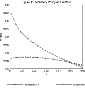
Figure 11 plots welfare against a range of values forψ.Thisfigure shows the behaviour

of welfare for the case of endogenous price flexibility. As a point of comparison, it also

shows a plot of welfare for the case where price flexibility is exogenouslyfixed at a given

level. In this example we setγ = 0.75.The exogenousγ case corresponds to the standard

model widely analysed in the literature on optimal monetary policy (see e.g. Benigno and

Woodford (2005)) and it is therefore a natural point of comparison.

The welfare plot for the exogenousγ case shows that the optimal value ofψis

approx-imately0.012. This implies that it is optimal for monetary policy to allow some volatility

in inflation in order to achieve some stabilisation of the welfare-relevant output gap. This

corresponds to the result emphasised by Benigno and Woodford (2005). This result is

quite standard and is analysed and explained in detail by Benigno and Woodford (2005).

In essence, cost-push shocks of the type assumed in this model, are distortionary and

imply that the flexible price equilibrium is sub-optimal. In a sticky price environment it

is therefore not optimal for monetary policy to reproduce the flexible price equilibrium.

Sticky prices give monetary policy some degree of leverage which can be used to stabilise

output around the welfare maximising level. This requires some volatility in inflation.

In terms of the policy rule of the form assumed in this model, it is optimal for ψ to be

The second plot in Figure 11 shows welfare when price flexibility is endogenous. The

parameter values and the relationship between ψ and the equilibrium value of γ are as

shown in Figure 10 (although the range of values of ψ shown in Figure 11 is narrower

than in Figure 10). It is immediately clear from Figure 11 that, in the endogenous price

flexibility case, welfare appears to increase monotonically asψdecreases towards zero. In

other words, when price flexibility is endogenous, it appears to be optimal to engage in

strict inflation stabilisation. This is in complete contrast to the case of exogenous price

flexibility, as analysed by Woodford (2003) and Benigno and Woodford (2005), where it

is optimal to allow some variability in inflation.

The contrast between the two cases arises for two reasons. Firstly, as ψ is reduced,

the rise in the equilibrium value of γ reduces the resource cost of price flexibility (i.e.

fewer price changes imply lower costs). Secondly, the rise in the equilibrium value of

γ implies that monetary policy becomes a more effective policy tool (because the real

effects of monetary policy depend on the presence of nominal rigidities and these become

more significant asγ increases). Therefore, asγ increases, monetary policy becomes more

effective in dealing with the distortions caused by cost-push shocks. This is reflected in a

higher level of welfare as ψ decreases andγ increases.

This result represents a significant departure compared to the literature based on

exogenous price flexibility. That literature has emphasised that complete inflation

stabil-isation is not optimal in the face of cost-push shocks. The comparison shown in Figure

11 implies that this result may be overturned when price flexibility is endogenised.

Of course, Figure 11 is based on just one set of parameter values. Nevertheless,

experiments (not reported) testing the sensitivity of this basic qualitative result indicate

that it is robust across a wide range of values for key parameters, such as φ, μand ρ.

The results described above focus entirely on the implications of cost-push shocks.

Woodford (2003) and Benigno and Woodford (2005), using models with exogenous price

terms of their implications for optimal monetary policy. This similarity carries over into

our model, so extending our results to consider shocks toGadd no significant new insights.

Extending our analysis to consider labour supply shocks (i.e. shocks to K in our model)

also adds little. Woodford (2003) and Benigno and Woodford (2005), using models of

exogenous priceflexibility, show that optimal monetary policy should completely stabilise

inflation in the face of labour supply shocks (i.e. policy should replicate the flexible price

equilibrium). In that case, our model of endogenous priceflexibility simply predicts that

prices will be completely rigid. This has no impact on the nature of optimal monetary

policy in the face of labour supply shocks.

6

Conclusion

This paper takes a standard sticky-price general equilibrium model and incorporates a

simple mechanism which endogenises the degree of nominal price flexibility. We show

how the degree of price flexibility is determined within the model and analyse the effects

of key parameter values on the equilibrium degree of priceflexibility. The analysis shows

that the equilibrium degree of price flexibility is sensitive to changes in monetary policy.

The more weight monetary policy places on the stabilisation of the output-gap, the more

flexible prices become. Conversely, the more weight monetary policy places on inflation

stabilisation, the more inflexible prices become. The paper also analyses welfare

maximis-ing monetary policy when the degree of price flexibility is endogenous. This is compared

to welfare maximising monetary policy in the case of exogenous priceflexibility. We show

that endogenising the degree of price flexibility tends to shift optimal monetary policy

towards complete inflation stabilisation, even when shocks take the form of cost-push

disturbances. This contrasts with the standard result obtained in models with exogenous

price flexibility, which show that optimal monetary policy should allow some degree of

Appendix A: Approximation of Producer

j

’s Utility

A second-order approximation of (29) is derived as follows. First substitute for yt(j) to

yield

˜

U0(j) = E0

∞ X

t=1

βt−1 "

Ct−ρYt µ

pt(j) Pt

¶1−φ

− χΛtKt

μ Y μ t

µ pt(j)

Pt

¶−φμ#

−₁ α

−β(1−γ(j)) (38)

which can be written as

˜

U0(j) = E0

∞ X

t=1

βt−1 "

α1,t µ

pt(j) Pt

¶1−φ

−α2,t µ

pt(j) Pt

¶−φμ#

− α

1₋β(1−γ(j)) (39)

where

α1,t =Ct−ρYt andα2,t=

χΛtKtYtμ μ

This form of the utility function isolates terms which depend on γ(j). A second order

approximation of (39) implies

˜

U0(j)−U¯ = C¯1−ρE0

∞ X

t=1

βt−1

∙ ˆ

α1,t− φ₋1

φμ αˆ2,t

−(φ−₂1)ζ(ˆpt(j)−Pˆt)2+

1 2αˆ

2 1,t−

φ₋1 2φμ αˆ

2 2,t

−(φ₋1)ˆα1,t(ˆpt(j)−Pˆt) + (φ−1)ˆα2,t(ˆpt(j)−Pˆt) i

(40)

−₁ α

−β(1−γ(j)) +O ¡

ε3¢

which can be simplified to

˜

U0(j)−U¯ = −

(φ₋1) 2 C¯

1−ρ_E

0

∞ X

t=1

βt−1hζ(ˆpt(j)−Pˆt)2

−2(ˆα2,t−αˆ1,t)(ˆpt(j)−Pˆt) i

(41)

+tij₋ α

1₋β(1−γ(j)) +O ¡

where tij represents terms independent of producer j. Note that

ˆ

α2,t−αˆ1,t = ˆΛt+ ˆKt+μYˆt+ρCˆt−Yˆt+O ¡

ε2¢

which, from (19) implies

ˆ

α2,t−αˆ1,t =ζ(ˆpot−Pˆt) +O ¡

ε2¢

so

˜

U0(j)−U¯ =

(φ₋1)ζ

2 C¯ 1−ρ_E

0

∞ X

t=1

βt−1h₋(ˆpt(j)−Pˆt)2

+2(ˆpo_{t −}Pˆt)(ˆpt(j)−Pˆt) i

(42)

+tij₋ α

1₋β(¯γ−γ(j)) +O ¡

ε3¢

which is equation (30) in the main text.

Appendix B: Expected Dynamics of Producer

j

’s Price

The first-order condition for price setting for producer j has the same form as (14) and

therefore implies

ˆ

xt(j) = (1−βγ(j))ˆpot +βγ(j)Et[ˆxt+1(j)] +O

¡ ε2¢

or

ˆ

xt(j)−Pˆt= (1−βγ(j))ˆpot −Pˆt+βγ(j)Et[ˆxt+1(j)−Pˆt] +O ¡

ε2¢ (43)

Using the relationship

Et[ˆxt+1(j)−Pˆt] =Et[ˆxt+1(j)−Pˆt+1] +Et[πt+1]

equation (43) can be written as

ˆ

xt(j)−Pˆt = (1−βγ(j))(ˆpot −Pˆt) +βγ(j)Et[ˆxt+1(j)−Pˆt+1] +βγ(j)Et[πt+1] +O

which is equation (31) in the main text.

The Calvo pricing process implies thatEC

0[ˆpt(j)−Pˆt]evolves according to the following equation

E₀C[ˆpt(j)−Pˆt] =γ(j)E0C[ˆpt−1(j)−Pˆt] + (1−γ(j))(ˆxt(j)−Pˆt) +O ¡

ε2¢ (44)

Using the relationship

E₀C[ˆpt−1(j)−Pˆt] =E0C[ˆpt−1(j)−Pˆt−1]−πt

equation (44) can be written as

E0C[ˆpt(j)−Pˆt] =γ(j)E0C[ˆpt−1(j)−Pˆt−1] + (1−γ(j))(ˆxt(j)−Pˆt)−γ(j)πt+O ¡

ε2¢

which is equation (33) in the main text.

An equation for the evolution of E0[(ˆpt(j)−Pˆt)2]can be derived in a similar way. First

note that the Calvo pricing process implies that

E0[(ˆpt(j)−Pˆt)2] =γ(j)E0[(ˆpt−1(j)−Pˆt)2] + (1−γ(j))E0[(ˆxt(j)−Pˆt)2] +O ¡

ε3¢ (45)

Using the relationships

E0[(ˆpt−1(j)−Pˆt)2] =E0[(ˆpt−1(j)−Pˆt−1)2] +E0[π2t]−2E0[πt(ˆpt−1(j)−Pˆt−1)]

and

E0[πt(ˆpt−1(j)−Pˆt−1)] =E0D[πtE0C(ˆpt−1(j)−Pˆt−1)]

equation (45) can be written as

E0[(ˆpt(j)−Pˆt)2] = γ(j)E0[(ˆpt−1(j)−Pˆt−1)2] +γ(j)E0[π2t]

−2γ(j)E0D[πtE0C(ˆpt₋1(j)−Pˆt₋1)]

+(1₋γ(j))E0[(ˆxt(j)−Pˆt)2] +O ¡

ε3¢

References

[1] Benigno, P. and M. Woodford (2005) “Inflation Stabilization and Welfare: The Case

of a Distorted Steady State”Journal of the European Economic Association,3,

1185-1236.

[2] Calmfors, L. and A. Johansson (2006) “Nominal Wage Flexibility, Wage Indexation,

and Monetary Union” Economic Journal, 116, 283-308.

[3] Calvo, G. A. (1983) “Staggered Prices in a Utility-Maximising Framework”Journal

of Monetary Economics, 12, 383-398.

[4] Clarida, R. H., J. Gali and M. Gertler (1999) “The Science of Monetary Policy: a

New Keynesian Perspective” Journal of Economic Literature, 37, 1661-1707.

[5] Devereux, M. B. (2006) “Exchange Rate Policy and Endogenous Price Flexibility”,

Journal of the European Economic Association, 4, 735—769.

[6] Devereux, M. B. and H. E. Siu (2007) “State Dependent Pricing and Business Cycle

Asymmetries”International Economic Review, 48, 281-310.

[7] Devereux, M. B. and D. Yetman (2002) “Menu Costs and the Long Run

Output-Inflation Trade-off” Economic Letters, 76, 95-100.

[8] Devereux, M. B. and D. Yetman (2003)“Price-Setting and Exchange Rate

Pass-Through: Theory and Evidence” in Price Adjustment and Monetary Policy:

Pro-ceedings of a Conference Held by the Bank of Canada, Bank of Canada Publications,

347-371.

[9] Devereux, M. B. and D. Yetman (2010)“Price Adjustment and Exchange Rate

[10] Dotsey, M. and R. G. King (2005) “Implications of State-Dependent Pricing for

Dynamic Macroeconomic Models” Journal of Monetary Economics, 52, 213-242.

[11] Dotsey, M., R. G. King and A. L. Wolman (1999) “State Dependent Pricing and

the General Equilibrium Dynamics of Money and Output” Quarterly Journal of

Economics, 114, 655-690.

[12] Golosov, M. and R. E. Lucas (2007) “Menu Costs and Phillips Curves” Journal of

Political Economy, 115, 171-199.

[13] Levin, A. and T. Yun (2007) “Reconsidering the Natural Rate Hypothesis in a New

Keynesian Framework” Journal of Monetary Economics, 54, 1344-1365.

[14] Kiley, M. T. (2000) “Endogenous Price Stickiness and Business Cycle Persistence”

Journal of Money, Credit and Banking, 32, 28-53.

[15] Romer, D. (1990) “Staggered Price Setting with Endogenous Frequency of

Adjust-ment”Economics Letters, 32, 205-210.

[16] Senay, O. and A. Sutherland (2006) “Can Endogenous Changes on Price Flexibility

Alter the Relative Welfare Performance of Exchange Rate Regimes?” inNBER

Inter-national Seminar on Macroeconomics 2004 R. H. Clarida, J. F. Frankel, F. Giavazzi

and K. D. West (eds.), MIT Press, 371-400.

[17] Woodford, M. (2003) Interest and Prices: Foundations of a Theory of Monetary

Policy Princeton University Press.

[18] Yetman, J. (2003) “Fixed Prices versus Predetermined Prices and the Equilibrium

0 0.2 0.4 0.6 0.8 1 0

0.1 0.2 0.3 0.4 0.5 0.6 0.7 0.8 0.9 1

Figure 1: Price Adjustment Costs and the Best Response Function

γ

γ

(j)

α=0.00001 α=0.0001 α=0.00055 α=0.0015 α=0.005

0 0.5 1 1.5 2 2.5 3

x 10-3 0

0.1 0.2 0.3 0.4 0.5 0.6 0.7 0.8 0.9

1 Figure 2: Price Adjustment Costs and Equilibrium γ

α

Equilibr

ium

0 0.2 0.4 0.6 0.8 1 0

0.1 0.2 0.3 0.4 0.5 0.6 0.7 0.8 0.9

1 Figure 3: φ and the Best Response Function

γ

γ

(j)

φ=4 φ=8 φ=12

4 6 8 10 12 14

0 0.1 0.2 0.3 0.4 0.5 0.6 0.7 0.8 0.9

1 Figure 4: φ and Equilibrium γ

φ

Equilibr

ium

0 0.2 0.4 0.6 0.8 1 0

0.1 0.2 0.3 0.4 0.5 0.6 0.7 0.8 0.9

1 Figure 5: μ and the Best Response Function

γ

γ

(j)

μ=1 μ=1.5 μ=3

1 1.5 2 2.5 3 3.5 4 4.5 5 0

0.1 0.2 0.3 0.4 0.5 0.6 0.7 0.8 0.9

1 Figure 6: μ and Equilibrium γ

μ

Equilibr

ium

0 0.2 0.4 0.6 0.8 1 0

0.1 0.2 0.3 0.4 0.5 0.6 0.7 0.8 0.9

1 Figure 7: ρ and the Best Response Function

γ

γ

(j)

ρ=0.5 ρ=1 ρ=2

0.5 1 1.5 2 2.5 3 3.5 4 4.5 5 0

0.1 0.2 0.3 0.4 0.5 0.6 0.7 0.8 0.9

1 Figure 8: ρ and Equilibrium γ

ρ

Equilibr

ium

0 0.2 0.4 0.6 0.8 1 0

0.1 0.2 0.3 0.4 0.5 0.6 0.7 0.8 0.9

1 Figure 9: ψ and the Best Response Function

γ

γ

(j)

ψ=0.01 ψ=0.05 ψ=0.3

0 0.1 0.2 0.3 0.4 0.5 0

0.1 0.2 0.3 0.4 0.5 0.6 0.7 0.8 0.9

1 Figure 10: ψ and Equilibrium γ

ψ

Equilibr

ium

0 0.01 0.02 0.03 0.04 0.05 0.06 0.02

0.025 0.03 0.035 0.04 0.045 0.05 0.055

0.06 Figure 11: Monetary Policy and Wefare

Welfar

e

ψ

www.st-and.ac.uk/cdma

ABOUT THECDMA

The Centre for Dynamic Macroeconomic Analysis was established by a direct grant from the University of St Andrews in 2003. The Centre funds PhD students and facilitates a programme of research centred on macroeconomic theory and policy. The Centre has research interests in areas such as: characterising the key stylised facts of the business cycle; constructing theoretical models that can match these business cycles; using theoretical models to understand the normative and positive aspects of the macroeconomic policymakers' stabilisation problem, in both open and closed economies; understanding the conduct of monetary/macroeconomic policy in the UK and other countries; analyzing the impact of globalization and policy reform on the macroeconomy; and analyzing the impact of financial factors on the long-run growth of the UK economy, from both an historical and a theoretical perspective. The Centre also has interests in developing numerical techniques for analyzing dynamic stochastic general equilibrium models. Its affiliated members are Faculty members at St Andrews and elsewhere with interests in the broad area of dynamic macroeconomics. Its international Advisory Board comprises a group of leading macroeconomists and, ex officio, the University's Principal.

Affiliated Members of the School

Dr Fabio Aricò. Dr Arnab Bhattacharjee. Dr Tatiana Damjanovic. Dr Vladislav Damjanovic. Prof George Evans. Dr Gonzalo Forgue-Puccio. Dr. Michal Horvath Dr Laurence Lasselle. Dr Peter Macmillan. Prof Rod McCrorie. Prof Kaushik Mitra. Dr. Elisa Newby

Prof Charles Nolan (Director). Dr Geetha Selvaretnam. Dr Ozge Senay. Dr Gary Shea. Prof Alan Sutherland. Dr Kannika Thampanishvong. Dr Christoph Thoenissen. Dr Alex Trew.

Senior Research Fellow

Prof Andrew Hughes Hallett, Professor of Economics, Vanderbilt University.

Research Affiliates

Prof Keith Blackburn, Manchester University. Prof David Cobham, Heriot-Watt University. Dr Luisa Corrado, Università degli Studi di Roma. Prof Huw Dixon, Cardiff University.

Dr Anthony Garratt, Birkbeck College London. Dr Sugata Ghosh, Brunel University.

Dr Aditya Goenka, Essex University. Dr Michal Horvath, University of Oxford. Prof Campbell Leith, Glasgow University. Prof Paul Levine, University of Surrey. Dr Richard Mash, New College, Oxford.

Dr Gulcin Ozkan, York University.

Prof Joe Pearlman, London Metropolitan University. Prof Neil Rankin, Warwick University.

Prof Lucio Sarno, Warwick University.

Prof Eric Schaling, South African Reserve Bank and Tilburg University.

Prof Peter N. Smith, York University. Dr Frank Smets, European Central Bank. Prof Robert Sollis, Newcastle University. Prof Peter Tinsley, Birkbeck College, London. Dr Mark Weder, University of Adelaide.

Research Associates

Mr Nikola Bokan. Mr Farid Boumediene. Miss Jinyu Chen. Mr Johannes Geissler. Mr Ansgar Rannenberg. Mr Qi Sun.

Advisory Board

Prof Sumru Altug, Koç University. Prof V V Chari, Minnesota University. Prof John Driffill, Birkbeck College London.

Dr Sean Holly, Director of the Department of Applied Economics, Cambridge University.

Prof Seppo Honkapohja, Bank of Finland and Cambridge University.

Dr Brian Lang, Principal of St Andrews University. Prof Anton Muscatelli, Heriot-Watt University. Prof Charles Nolan, St Andrews University.

Prof Peter Sinclair, Birmingham University and Bank of England.

Prof Stephen J Turnovsky, Washington University. Dr Martin Weale, CBE, Director of the National

www.st-and.ac.uk/cdma RECENTWORKINGPAPERS FROM THE

CENTRE FORDYNAMICMACROECONOMICANALYSIS

Number Title Author(s)

CDMA08/03 Exchange rate dynamics, asset market structure and the role of the trade elasticity

Christoph Thoenissen (St Andrews)

CDMA08/04 Linear-Quadratic Approximation to Unconditionally Optimal Policy: The Distorted Steady-State

Tatiana Damjanovic (St Andrews), Vladislav Damjanovic (St Andrews) and Charles Nolan (St Andrews) CDMA08/05 Does Government Spending Optimally

Crowd in Private Consumption? Michal Horvath (St Andrews)

CDMA08/06 Long-Term Growth and Short-Term

Volatility: The Labour Market Nexus Barbara Annicchiarico (Rome), LuisaCorrado (Cambridge and Rome) and Alessandra Pelloni (Rome)

CDMA08/07 Seigniorage-maximizing inflation Tatiana Damjanovic (St Andrews) and Charles Nolan (St Andrews)

CDMA08/08 Productivity, Preferences and UIP deviations in an Open Economy Business Cycle Model

Arnab Bhattacharjee (St Andrews), Jagjit S. Chadha (Canterbury) and Qi Sun (St Andrews)

CDMA08/09 Infrastructure Finance and Industrial

Takeoff in the United Kingdom Alex Trew (St Andrews)

CDMA08/10 Financial Shocks and the US Business

Cycle Charles Nolan (St Andrews) andChristoph Thoenissen (St Andrews)

CDMA09/01 Technological Change and the Roaring

Twenties: A Neoclassical Perspective Sharon Harrison (Columbia) MarkWeder (Adeleide)

CDMA09/02 A Model of Near-Rational Exuberance George Evans (Oregon and St Andrews), Seppo Honkapohja (Bank of Finland and Cambridge) and James Bullard (St Louis Fed) CDMA09/03 Shocks, Monetary Policy and

Institutions: Explaining Unemployment Persistence in “Europe” and the United States

Ansgar Rannenberg (St Andrews)

CDMA09/04 Contracting Institutions and Growth Alex Trew (St Andrews)