State Dependent Choice
∗
Paola Manzini
†University of St Andrews and IZA
Marco Mariotti
‡Queen Mary University of London
April 2015
Abstract
We propose a theory of choices that are influenced by the psychological state of the agent. The central hypothesis is that the psychological state controls theurgency of the attributes sought by the decision maker in the available alternatives. While state dependent choice is less restricted than rational choice, our model does have empirical content, expressed by simple ‘revealed preference’ type of constraints on observable choice data. We demonstrate the applicability of simple versions of the framework to economic contexts. We show in particular that it can explain widely researched anomalies in the labour supply of taxi drivers.
JEL codes:D01.
Keywords:Bounded rationality, procedural rationality, utility maximization, choice behavior.
∗This paper radically revises and supersedes a previous paper entitled ‘Moody Choice’. We are grateful for helpful comments to two anonymous referees, the Editor in charge Clemens Puppe, Attila Ambrus, Sophie Bade, Nick Baigent, Vince Crawford, Stephan Dickert, Yorgos Gerasimou, Andreas Gloeckner, Steffen Huck, Silvia Milano, Mauro Papi, Daniel Sgroi, Chris Tyson, Lin Zhang as well as several seminar audiences. We’ve had numerous inspiring discussions with Michael Mandler on related topics. Financial support through ESRC grant RES-000-22-3474 is gratefully acknowledged.
†School of Economics and Finance, University of St. Andrews, Castlecliffe, The Scores, St. Andrews
KY16 9AL, Scotland, U.K. (e-mail: [email protected]).
‡School of Economics and Finance, Queen Mary University of London, Mile End Road, London E1
1
Introduction
In this paper we propose a theory of choices that are influenced by the psychological state in which the decision is taken. We wish to avoid as much as possible to commit to any specific psychological phenomenon. To do so, we imagine that an agent makes decisions by looking at the alternatives as carriers of attributes, or properties. This is fairly standard and is consistent with the Lancaster [36] tradition of consumer theory, with modern approaches to empirical demand analysis (e.g. Berry, Levinsohn and Pakes [6]) and with other abstract modern theories of choice (e.g. Dietrich and List [15]).
What gives leverage to our theory is the assumption that properties are looked at sequentially by the agent. For example, when searching for a restaurant, the agent may first check only the restaurants that are nearby, then focus on the French ones among these, then see whether there is any nearby French with acceptable prices, and so on. In general, following a list of desirable properties, the agent progressively eliminates at each stage alternatives that do not possess the relevant property, until a set of ac-ceptable alternatives is found.1 This is a case of ‘sequentially rationalisable choice’ (Manzini and Mariotti [41]) and we showed in Mandler, Manzini and Mariotti [40] (henceforth MMM) that the decisions resulting from this type of procedure are indis-tinguishable from those of a standard utility maximising agent. In other words, MMM cannot explain any violation of the Weak Axiom of Revealed Preference (WARP). Thus, while it has the methodological value of providing a procedural foundation for utility maximisation, the MMM model does not go beyond the standard model in terms of the phenomena it can explain. In this paper, we extend the explanatory power of the MMM model by dropping the assumption that the order in which the properties are applied is fixed. So, to continue with the restaurant example, we allow the agent to consider as the most urgent property sometimes price, sometimes the type of cuisine, and sometimes the location, as well as to have sometimes more drive for one type of cuisine and sometimes for others. Or, we allow an investor to sometimes look first at the safety features of an investment and some other times (perhaps in an irrationally exuberant mood) to consider the maximum return as the most important property. In this way, while obtaining a theory that is not vacuous, we are able to capture inter-esting types of ‘non-standard’ behaviour that are determined by a psychological state,
1See Mandler, Manzini and Mariotti [40] for a discussion of the psychological foundations of this
modelled as the relative urgency of the properties sought by the agent. Furthermore, the theory becomes sufficiently flexible to be applied to economics settings in a fruit-ful way, explaining some observed anomalies that are difficult to accommodate in the standard utility maximisation model.
That the psychological state of the agent has an effect on the cognitive process un-derlying choice is intuitive and is an increasingly accepted feature of economic models. For example, the relationship between ‘mood’ and choice is documented in an impres-sively large body of empirical evidence from psychology and economics.2 In the large literature on menu choice (Kreps [34]; Dekel, Lipman and Rustichini [14]), an agent anticipates being in one of different preference determining states. And there exist several models of the effects on choice of specific psychological states, such as ‘antic-ipatory feelings’ (Caplin and Leahy [8]). In the MMM model the cognitive process underlying choice is summarised by the order in which properties are applied. There-fore, if it is granted that psychological states do matter, it is natural to take the order of the relevant properties as a variable rather than a fixed element of the model.
One of our main aims is to arrive at a general, flexible framework to incorporate the effects of the disparate psychological factors affecting choice, with a view to teasing out the empirical restrictions entailed by the dependence on these factorsper se(that is, in-dependently of the specificity of the factor). One ‘natural’ approach might appear that of using a state dependent utility function. However, one difficulty of this approach is that it has an empty empirical content when states depend on choice menus (see section 6). For this reason, while still avoiding to commit to a specific interpretation of what a psychological state is, we use the richer primitives of the MMM model rather than the behaviourally equivalent utility maximisation model. By doing so, we ob-tain a framework in which behaviour always presents systematic patterns even when subject to psychological influences. Such patterns can be identified by means of direct observation of choice data, through tests that are simple variations of standard tests in revealed preference theory.
We callmindsetthe set of properties considered in general by the agent, ‘the things that make the agent tick’. A glutton would have to change his mindset/personality, not just the contingent factors affecting choice, to start paying attention to the fat content of his diet. A foolhardy agent will always ignore the safety aspects of his options. While the mindset is fixed throughout all choices, how the relevant properties are ranked
2A sample of publications is: Capra [10], Erber et al. [19], Ifcher and Shaghaghi [26] Isen [27], Kahn
with respect to one another can vary. We call the order in which properties are con-sidered astate. This methodology allows us to describe an agent with a recognisable identity (in the form of a fixed set of values) who makes different choices in different conditions: an alternative with the property that is top in a state might be selected in that state, but discarded in a state that prioritises different properties that this alterna-tive does not possess.
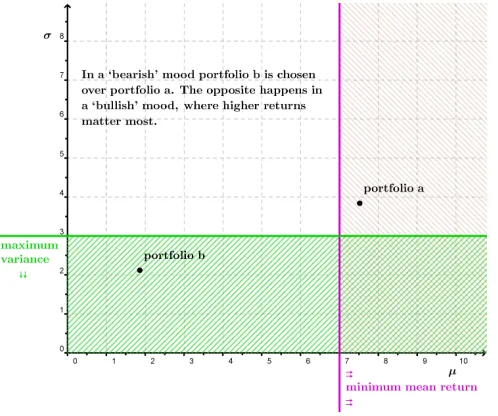
[image:4.612.94.343.328.536.2]To give a flavour of how the model works, the investor depicted in Figure 1 can be in two states, bearish or bullish. His mindset consists of just two ‘threshold’ proper-ties: minimum acceptable return and maximum acceptable risk. In a bearish state, the investor puts risk limitation at the forefront and selects portfolio b, which is the only one of the two to have the relevant property, while in a bullish state she looks first for a minimum return, selecting portfolioa.
Figure 1:Bulls and bears
This cognitive process under-lying choice extends to situa-tions with more numerous and more complex properties.
How are states determined? We consider two models that capture two distinct plausible possibilities. In the first model, a state ismenu driven, that is, trig-gered by the menu under con-sideration. This is a most natural situation in consumer choice, as sellers may and do manipulate menus to their advantage (e.g. using “asymmetric dominance” effects), but it may occur in other contexts too. For example, if an agent finds it costly to contemplate a menu before selecting an alternative from it (e.g. Ergin and Sarver [20]), menus with different con-templation costs may induce different states.
for risk and hence makes the ‘high return property’ the more urgent one. The environ-mental state model assumes that, as in most cases outside controlled experiments, we cannot observe the state of an agent making a choice.
We show that the model in which states are menu driven is equivalent to choice data satisfying a single property (Togetherness). An interesting aspect of this property is that it is intermediate in strength between two textbook properties: it is weaker than the Weak Axiom of Revealed Preference (WARP) and stronger than Sen’s property β
(section 3). Concretely, think of a competitive consumer choosing from budgets. To-getherness says that all those bundles that are acceptable at some budget either remain (if still available) all acceptable or become all unacceptable following a price/income change. Togetherness implies in particular that an agent who reveals himself willing to engage in asequence of trades, say leading from x toy, is also willing to engage in a direct trade between x and y. So in particular a welfare planner can still use such ‘revealed indifferences’ as a guidance, as he would with a standard agent.
The second model, where states are environment driven, admits multiple obser-vations of choice from the same menu, made in different states. We show that the set of possible choice observations (in all possible states) fails Independence of Irrele-vant Alternatives and other consistency properties, yet is again fully characterised by a single property (state dependent WARP, or sd-WARP) that is intermediate between two standard properties: it is weaker than WARP and stronger than Sen’s Propertyα.
Once again, consider a competitive consumer. sd-WARP states in that context that if a bundle is always (i.e. in any state) rejected at some prices and income(p,M), then it is always rejected at any other budget for which allthe bundles demanded (in some state) at(p,M)are affordable (section 4).
An advantage of the axiomatic approach is that it automatically generates a recipe for direct empirical tests of the theory. Secondly, it permits simple and sharp be-havioural distinctions between our theory and other axiomatic theories of psycholog-ically driven choice, even using a very limited range of menus and observations. In this vein, we show how to distinguish between our model and a model of indecisive
behaviour (section 6.3).
Though abstract, our framework is workable and can yield novel economic in-sights. In section 5 we specialise the models to use them in a specific economic settings. We look at a long-standing debate on labour supply responses by workers who (like taxi-drivers) can choose their supply in a non-lumpy way.3Even a very stripped down
version of the model (that postulates ‘target-driven’ behaviour as suggested in the em-pirical literature) can accommodate the ‘anomaly’ of negative wage elasticities. The new key insight we provide lies in the asymmetry between income targets, which can be ‘unrealistic’, and leisure targets, which have a physical bound (there are so many hours in a day). This interplay means in the model that workers can display a whole range of wage elasticities depending on the magnitude of wage changes and inde-pendently of any role of expectations (which conversely play a key role in reference-dependent explanations). This application also yields two novel empirically testable predictions. Similar simplifications of the theory can be easily applied to saving deci-sions and consumer theory.
2
Mindset and states
Fix a finite set of alternativesX. Given the collectionΣ of all nonempty subsets ofX, a choice function is a correspondence c that associates with each A ∈ Σ (a menu) a nonempty set c(A) ⊆ A, the agent’s observed selection from A. To build a model of state dependent choice, we begin by assuming, as in Mandler, Manzini and Mariotti [40] (MMM), that the agent makes choices by sequentially going through a checklist of ‘properties’ of alternatives (properties are intended as synonymous with ‘attributes’). At each step, he discards the alternatives that lack the relevant property. In spite of it being procedural (it is a particular case of procedures such as sequential rationalis-ability as in Manzini and Mariotti [41] and those in Apesteguia and Ballester [4]), this decision model is shown in MMM to be equivalent to ordinary preference maximisa-tion: an agent has a checklist if and only if he maximises a preference relation. Any checklist corresponds to a preference, and vice versa. However the checklist model has richer primitives than ordinary preference maximisation. This feature permits to dis-tinguish, unlike a preference, between the more stable traits of the agent’s personality (mindset), and the more variable aspects (states).
We identify a property with the set of alternatives that possess that property. So formally a property is a subset P ⊆ X, and we say that x has property P whenever
x ∈ P. E.g. the property ‘sweet’ consists of all the objects in X which are sweet. A
mindsetΓ⊆2X\∅is a set of mutually distinct properties. A mindsetΓisnestedif for
allP,Q∈ Γwe have eitherP ⊆QorQ ⊆P. Given a mindsetΓ, astateis a strict linear order<ofΓ.
which a choice is made is not necessarily observable: only the resulting choice is.
3
The state is determined by the menu
In our first model the state is triggered by the menu. Multiple choices from a menu are allowed, and they are interpreted as being made always in the same state (the one triggered by the menu itself). Given a mindset Γ and a menu A ∈ Σ, denote by <A
the state induced by A (which we refer to as ‘a state for A’). Denote by P0A the first property in state<A(the<A −least element ofΓ).4
A menu checklist is a pair Γ,{<A}A∈Σ
of a mindset and a collection of states, one for each menu. Given A ∈ Σ and a menu checklist Γ,{<A}A∈Σ
, we can define inductively a series of ’survivor sets’:
SA
P0A,<A =A
and
For allP ∈ Γ\P0A: SA(P,<A) =
\
Q<AP
SA(Q,<A)∩P if \
Q<AP
SA(Q,<A)∩P6=∅
\
Q<AP
SA(Q,<A) otherwise
That is, when facing the menu A, the agent’s state for that menu identifies the order of the properties in the checklist. The agent scans the checklist, and when considering each property he only retains the alternatives which have that property, if any. Other-wise he retains all the alternatives that have survived until that stage. Then the agent moves to next stage. When convenient we omit denoting the linear order in the sets
SA(P,<A)and simply writeSA(P).
Definition 1 A choice function c on Σ is a menu driven state dependent choice if there exists a menu checklist Γ,{<A}A∈Σ
such that for all A∈ Σ, for some property P ∈ Γ,
SA(P) = SA(Q)for all Q ∈ Γwith P <A Q
c(A) = SA(P) (1)
4While in this paper we confine ourselves to finite sets, the definitions are written so as to
In words, a menu driven state dependent choice is such that all those alternatives that are chosen from a menu are in the ‘last’ survival set constructed on the basis of the relevant state for that menu.
While each menu triggers a different order in which the various properties are con-sidered, MMM consider checklists that are independent of the menu. A choice function
c onΣhas a checklist(Γ,<)if it is a menu driven state dependent choice with menu checklist Γ,{<A}A∈Σsuch that<A=<B=<for allA,B ∈ Σ. It turns out that a
check-list expresses the standard notion of rationality in economics, preference maximisation. A choice functionc maximises a preference if there exists a weak order5 %on Xsuch that, for allA∈ Σ,c(A) = {x : x%yfor ally ∈ A}:
Proposition 1 (MMM, [40]): A choice function c has a checklist if and only if it maximises a preference.6
A choice function may be a menu driven state dependent choice even if it has no checklist (see appendix 1). In light of the above proposition, this means that the model we propose can explain behaviour that is not preference maximising. The following example illustrates:
Example 1 A consumer enters an ‘exuberant’ state when he faces large menus or menus com-posed entirely of luxury items, but is in a thrifty state when a thrifty item is available in a small menu. As a consequence he will for instance choose an expensive food item from a hefty restaurant list, and a modest entree from a shorter one. Formally, let X = {x,y,z}, where x and y are luxury items, z is thrifty, and only the grand menu is large. So
c(X) =c({x,y}) = {x,y} and c({x,z}) =c({y,z}) ={z}
The choice function c cannot maximise any weak order (c(X) = {x,y} would imply x % z while c({x,z}) = {z} would imply z x) and therefore by Proposition 1 it cannot have a checklist. Nevertheless it is a menu driven state dependent choice with the menu checklist
({{x,y},{z}},<A)and states{x,y} <A {z} for A ∈ {X,{x,y}}and{z} <A {x,y}for A∈ {{x,z},{y,z}}.
We also make at this stage an observation that may appear surprising: in spite of the fact that each checklist corresponds to a preference, it isnotnecessarily the case that
5A weak order is a a complete transitive relation.
6This result is proved in MMM in greater generality than for the domain considered here. The
an agent who maximises a menu dependent preference is captured by a menu driven state dependent choice. This implies that the model does have empirical restrictions (unlike the model of menu dependent preferences). Details are in section 6.
3.1
Menu driven state dependence may not manifest itself in
be-haviour
State variations are not necessarily expressed in observable choice behaviour. In par-ticular, a necessary condition for state changes to be observable is that the properties cannot be ranked as more or less permissive, i.e., they arenot nested.
Example 2 There are two properties you look at when selecting from a restaurant menu: ‘rec-ommended by a friend’ and cheapness (all dishes are sufficiently appealing). The rice dish (r) has been recommended by a friend, while steak (s) and tacos (t) have not been recommended. Rice and tacos are cheap and steak is not. In a trusting state (the recommendation first springs to mind) rice is selected over both tacos and steak, and tacos are selected over fish. But evidently in a conservative state (cheapness first), you would make exactly the same choices! (Rice and tacos survive the first cheapness test and then rice is selected on the basis of the recommendation). Formally,
c({r,s,t}) =c({s,r}) =c({r,t}) =r and c({s,t}) =t
and the data are explained by the mindset{{r},{r,t}}both in the state{r} <A {r,t} for all A and in the ‘opposite’ state{r,t}<A {r}for all A.
This fact holds in general: when the mindset is nested, the state does not affect choice, an agent affected by states behaves exactly like one that is not (but has the same mindset).
Proposition 2 Let c be a menu driven state dependent choice with nested mindset. Then c maximises a preference.
keeps all of them. In the next stage he revises the satisfaction threshold. There is no need to specify the revision rule, precisely because the properties are nested. The best alternatives in a menu will never be eliminated: if, when considering a propertyP, the set of survivors from the previous stages contains some alternatives that are inP, then the best alternatives must be among them. The state, in this interpretation, manifests itself in the initial propertyt1and the revision rule adopted: sometimes the agent will
start with ambitious targets, and sometimes with more modest ones; sometimes he will react to the lack of satisfactory alternatives by radically revising down the target, and sometimes he will hold firm. This agent is procedural as well as subject to state changes but his choice behaviour never appears to an external observer to be swayed by this instability!
[image:10.612.97.341.361.552.2]But the invariance of choice to state changes does not necessarily rest on nested states. In specific economic settings there are natural non-nested properties that - at least within a parameter range - generate choice invariance.
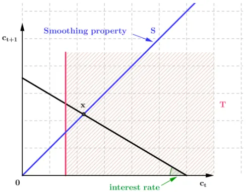
Figure 2:State dependent intertemporal consumption
In Figure 2 a saver in the standard consumption today and tomorrow (ct,ct+1) space
con-siders first two properties: in-tertemporal consumption smooth-ing (S, the 450line) and satisfac-tion of immediate urges (all con-sumption patterns to the right of the vertical line, the set T). For the interest rate indicated (and all those sufficiently close to it), choice is invariant to whether S
is applied beforeT or viceversa, and is always the pointx.
3.2
The observable behavioural implications of menu driven state
dependence
Once we step aside of the special cases studied in the previous section, however, menu driven state dependence does effect choices that cannot be rationalised in a standard manner.
Example 3 Rice (r) and tacos (t) are both choosable when steak (s) is also available, but rice alone is chosen over tacos when these are the only two available dishes. Formally
c({r,s,t}) ={r,t} and c({r,t}) = {r}
The choice from {r,t} implies that, if there existed a menu checklist for c, then its mindset would contain a property P which ‘separates’ r and t, i.e. r∈ P and t∈/ P. But then, whatever the state, such a property would sooner or later also separate r and t in{r,s,t}, contradicting r,t∈ c({r,s,t}).
The reasoning in the above example suggests a necessary property:
Togetherness: If an alternative xis rejected from a menu from which another alterna-tiveyis chosen, thenxcannot be chosen whenyis chosen. Formally, for all A,B ∈ Σ:
[x∈ A\c(A),y∈ c(A),y ∈ c(B)]⇒ x∈/ c(B).
This property is equivalent to saying that if xand yare both chosen from a menu, then from any other menu x and y are either both chosen or both rejected, hence the name Togetherness. It is intermediate in strength between two classical revealed pref-erence properties: the Weak Axiom of Revealed Prefpref-erence (WARP) and property β.
These are defined as follows:
WARP: If an alternative x is rejected from a menu from which another alternative y
is chosen, then x cannot be chosen when y is available. Formally: For all A,B ∈ Σ:
[x∈ A\c(A),y∈ c(A),y ∈ B] ⇒x ∈/ c(B).
Propertyβ: If an alternativexis rejected from a menu from which another alternative
y is chosen, then x cannot be chosen from a smaller menu from which y is chosen. Formally, for allA,B ∈ Σ: [B⊂ A, x∈ A\c(A),y∈ c(A),y ∈ c(B)]⇒ x∈/ c(B).
While apparently weak, Togetherness is fairly restrictive. For example, beside being stronger than Property β as noted, it is also (strictly) stronger than a natural variant
of WARP introduced by Ehlers and Sprumont [17], which requires that if the agent choosesxand rejectsyfrom a menu, then he cannot chooseyand rejectxfrom another menu.7
It turns out that Togetherness fully characterises our model.
Proposition 3 A choice function is a menu driven state dependent choice if and only if it satisfies Togetherness.
This result clarifies the sense in which our model yields testable conditions for state dependent behaviour. An agent, no matter how state dependent, will never be ob-served to accept two alternatives from one menu while rejecting only one of the two from another menu. And conversely, every time that this pattern is not observed we can explain observed choices by means of the model. Suppose I’m willing to go to the theatre or to the cinema when the only other alternatives are to work or to keep the appointment with the dentist, but choose to keep the appointment with the dentist when the other alternatives are cinema, theatre, work, and a visit to a friend in the hospital. In this example we have a violation of WARP but not of Togetherness: the switch from the choice of cinema or theatre to the choice of seeing the dentist can be imputed to a shift in state. It could be, for instance, that the presence of a friend in the hospital, while not providing me with a sufficiently strong reason to visit her, puts me in a pensive mood, focussing my mind away from entertainment choices.8
Any single-valued choice function satisfies Togetherness, so Proposition 3 does not impose testable restrictions on this type of data. However, the result applies to the most abstract version of the theory, with no restriction on how states may depend on menus. It is not difficult to build specialisations of the theory which are restric-tive even for single-valued choice data. A first example comes from Proposition 2: if properties are nested, the theory can be falsified by single-valued choice data, through violations of WARP. A second quite natural example is a generalisation of the well-known ‘Luce and Raiffa’s dinner’, whereby the presence of frog’s legs on a menu trig-gers a change in preference. Suppose that a menu may or may not contain a ‘trigger’
7The easy proof of this assertion is left as an exercise for the reader.
8As it often happens, choice data alone cannot be the ultimate arbiter in the selection of the model.
alternative that alters the psychological state (beside the Luce and Raiffa dinner ex-ample, the presence of an expensive bottle of wine may make a diner more inclined to splash out, or noticing a high paying job advertisement may put a job applicant in the mood for more ambitious applications). Given an alternative t ∈ X define a trig-ger checklistas a menu checklist(Γ,{<t,<o})with two states, with state<t applying
to all menus A such that t ∈ A, and the ‘ordinary’ state <o applying whenever the
decision maker is choosing from a menu which does not contain the trigger alterna-tive (e.g. we can see <o as a ‘neutral’ state and <t as an ‘excited’ state). Call a menu
driven state dependent choice with a trigger checklist atrigger state dependent choice. There are single-valued choice functions which are not trigger state dependent choice. Consider for instance the choice function c defined on X = {x,y,w,z} asc(X) = w;
c(xyw) = x = c(xwz); c(xyz) = y = c(ywz); c(yz) = z. Recall that each checklist determines a preference order. Whichever order is applied to X must rankw above any other alternative; consequently a different order must be applied to all three-sets. Howeverc(xyw) = x=c(xwz)implies thatxranks above all other alternatives, while
c(xyz) = y=c(ywz)implies thatyranks above all other alternatives, a contradiction. In general, it easy to prove9that a choice function is a trigger state dependent choice if and only if it there exists an alternative that partitions the domain in two subsets such that WARP applies to each subdomain.10
The relation ≈introduced in the proof of Proposition 3 can be interpreted as ‘be-havioural indifference’:x ≈yrequiresxandyto be never separated by choice. A menu driven state dependent agent satisfies the transitivity of the behavioural indifference≈. So in particular he is willing to carry out in one step a trade, such as betweenxandy, when he has implicitly (via≈) revealed his willingness to carry out a sequence of pair-wise trades leading fromxtoy. Moreover he will be willing to carry out explicitly the implicit sequence of trades in any order. This is because the implicit trades which are acceptable to a menu driven state dependent agent are all and only the trades between alternatives that have exactly the same properties, and ‘having the same properties’ is a symmetric and transitive relation.11 Of course, alternatives can share the same
rele-9The proof is available from the authors.
10Formally,c must satisfy the following weakening of WARP, where for any alternativex ∈ Xwe
defineΣx={S⊆X:x∈S}andΣ¬x=Σ\Σx:
t-WARP (trigger WARP): There exists t ∈ X such that for i = x,¬x: For all A,B ∈ Σi:
[x∈ A\c(A),y∈c(A),y∈B]⇒x∈/c(B).
11Mandler [39] shows how indifference can be distinguished from incompleteness by observing the
vant properties and be physically different: for example, walking, cycling and taking a bus can all belong to a ‘cheap leisurely means of transport’ behavioural indifference class for an agent.
These observations are important for welfare analysis. Like in the standard case, a planner faced with the task of choosing between implementingxorymay let himself be guided by the sequences of behavioural indifferences of a possibly menu driven state dependent agent without fear of hurting the agent’s welfare. Unlike standard welfare analysis, the planner can no longer always use as a guide for welfare judge-ments the behavioural strict preferences if he suspects that the agent is menu driven state dependent. Nevertheless, some choices may provide information about strict welfare judgements. In the previous example, work isneverchosen, whereas all other three alternatives which are available in different states (and we know that the state has changed across menus since WARP has been violated) are chosen under at least one state. We deduce that, whatever the hierarchy of importance among the properties sought in the alternatives, work never offers a crucial property that some other alter-native does not offer, and there are crucial properties that other alteralter-natives offer but work does not. Work appears thus a good candidate to be declared welfare inferior to the other three alternatives available in both states. We cannot make the same inference regarding visiting a friend in the hospital, since such a choice was not available in the first state. This type of reasoning is a variant of Bernheim and Rangel’s [5] approach to ‘behavioural welfare economics’ (see Manzini and Mariotti [43] for a discussion on welfare and bounded rationality. See also Masatlioglu et al. [46] and Rubinstein and Salant [52]).
4
The state is determined by the environment
In our second model the state does not depend on the menu, but we allow several observations of choice from an A, each time in a different (unidentifiable) state.12 A mindset is as before a setΓof properties, and a state is a linear order<mofΓ. We allow
for the possibility that each observation is itself multivalued.
Specifically, let M be the set of states in which any menu A is considered. A pair
Γ,{<m}m∈M
is called anenvironmental checklist. Let γ(A,<m) denote the choice
fromAin state<m∈ M. Analogously to before,γ(A,<m)is determined by a sequence
12As in the previous section, our setup is static. Laibson [35] studies a dynamic model of what we
of successive eliminations. Denote byP0m the first property in state <m. The survivor
sets are defined by
SA(P0m,<m) = A
and
For allP ∈ Γ\P0m: SA(P,<m) =
\
Q<mP
SA(Q,<m)∩P if \
Q<AP
SA(Q,<m)∩P6=∅
\
Q<mP
SA(Q,<m) otherwise
Then, for allA ∈ Σ,γ(A,<m)is defined as follows:
γ(A, < m) = SA(P,<m), where P∈ Γis such that (2) SA(P, < m) = SA(Q,<m)for allQ ∈ Γwith P<m Q
We begin by noting that the functions γ(.,<m), which describe the observations
conditional on one state, are consistent in the sense that they satisfy IIA:
IIA: If some alternatives of a larger menu are still available in a smaller menu, the alternatives chosen from the smaller menu are the available ones which are chosen from the larger menu. Formally, for all A,B ∈ Σ: [A⊂ B,c(B)∩ A6=∅] ⇒ c(A) =
c(B)∩ A. Then:
Proposition 4 For all<m∈ M,γ(.,<m)satisfies IIA.
This result is implied by Proposition 1 and standard properties of preference max-imisation, but we also give a direct proof in the Appendix.13 Unfortunately, Propo-sition 4 is often not of practical use: although eachγ(.,<m) satisfies IIA, the specific
state in which choice was made is most likely unobservable, as an external observer can often be expected to have only choice data, not state data, available. Thus, the ob-jectc(A)is now interpreted as the collection of all the choices the agent makes from A
in all possible unobservable states:
13While we are working for simplicity in the full domain, so that IIA and WARP are equivalent, the
Definition 2 A choice function c is anenvironment driven state dependent choiceif there exists an environmental checklist Γ,{<m}m∈M
such that for all A∈ Σ
c(A) = [ <m∈M
γ(A,<m) for all A∈ Σ
Abstracting from the fact that the choicesγare generated here by a checklist and not
by a utility, this framework parallels Salant and Rubinstein’s [53] ‘choice with frames’ (or Bernheim and Rangel [5] similar framework of ‘choice with ancillary conditions’), where a choice correspondence is interpreted as including, for each A, all the single-valued choices made fromAin some frame. The definition here is similar, but we allow the choice in a state,γ(A,<m), to be multi-valued.14 This means that, at a substantive
level, the models differ, as there may not be a one-to-one correspondence between the frames and the states that explain a given set of observations. Details are in section 6.
4.1
Environment driven state dependence causes behaviour
incon-sistency
We search for standard ‘consistency’ properties that c may satisfy. First of all, it is easy to show that c does not inherit IIA from the γ(.,<m). Alternatives which are
not chosen, in any state, from a larger menu, may be chosen, in some state, from a smaller menu in which they are available. We illustrate this with an example which shows, more specifically, thatcfails to satisfy two classical basic consistency properties implied by IIA. One is Propertyβalready defined, and the other is:
Expansion: An alternative chosen from two menus must still be chosen when the two menus are merged. Formally, for allA,B∈ Σ: c(A)∩c(B)⊆c(A∪B).
Suppose there are three properties you look at when selecting from a restaurant menu: recommended by a friend, cheapness, and perceived appeal. Rice and steak have been recommended, rice and tacos are cheap, and steak and tacos are appealing. In a trusting state you sift through the properties in this order (first recommendation, then cheapness, then appeal). In a confident state you switch the order of the first and last property: you prefer to rely on your own judgement and the last thing you look at
14Below (section 6) we explore the relationship with Salant and Rubinstein’s [53] in more detail.
Bern-heim and Rangel [5] also allow choice to depend on information beyond the feasible set, although their focus is not on the properties ofcbut rather on the welfare inferences that could be made by observing
is friends’ recommendations.
So in a trusting state the steak, which has been recommended by a friend, is selected over the tacos, which have not been recommended. And the steak is also selected, in a confident state, over the rice dish, because the latter is less appealing.
However both tacos and rice are cheaper than steak. When all three dishes are on the menu, you are never observed to select steak (in violation of Expansion and Propertyβ). The reason is that when you are trusting, steak and rice, which have both
been recommended, survive the first elimination round and then rice is selected on the grounds of cheapness. And when you are confident, steak and tacos, which are both appealing, are shortlisted, to finally select the cheap tacos. Formally:
Claim 1 c does not satisfy Expansion, nor Propertyβ.
Obviously, since Togetherness is stronger than Property β, this result also shows
thatcfails Togetherness.
4.2
Consistency of environment driven state dependent choice
We now show that environment driven state dependent behaviour is nonetheless sub-ject to strong empirical restrictions. Of course if the mindset comprised only nested properties, we would have a result analogous to Proposition 2.
Proposition 5 Let c be an environment driven state dependent choice with a nested mindset. Then c maximises a weak order%on X.
Property α: All the alternatives chosen from a larger menu are still chosen when available in a smaller menu. Formally, for all A,B ∈ Σ: [A⊂B,c(B)∩ A6=∅] ⇒
c(B)∩ A⊆c(A).
As we shall see, ifcis an environment driven state dependent choice, it must satisfy Property α. Intuitively, if in some state you pick steamed salmon from a menu, it
means that in that state steamed salmon fulfils some crucial property which the other alternatives do not fulfil, and this will continue to be the case even in subsets of that menu. Yet propertyα is not sufficient to characterisec(see appendix B.1). We need a
sd-WARP:If an alternative x is rejected from a menu A, then x is rejected from any other menu that containsall the alternatives chosen in A. Formally, for all A,B ∈ Σ:
[x∈ A\c(A),c(A) ⊆B]⇒ x∈/c(B).
For example, if you were observed to choose sometimes seabass and sometimes a vegetarian meal, but never salmon, from a menu, then you will not choose salmon from any new menu that includes both seabass and the vegetarian meal. If your behaviour is determined by a state, it is easy to understand why this must be the case. Whatever state you are in, your choices from the old menu reveal that the first property that discerns between salmon and seabass (resp., the vegetarian meal) is such that seabass (resp., the vegetarian meal) has it while salmon lacks it.
WARP strengthens sd-WARP simply by replacing the entire choice set c(A) with
anyalternative contained in it. For a fully rational agent any chosen element is repre-sentative of the class of chosen elements, but not so for an environment driven state dependent agent. Note also that sd-WARP implies Propertyα(see appendix B.2). The
main result of this section is:
Proposition 6 A choice function c is an environment driven state dependent choice if and only if it satisfies sd-WARP.
Changes in mental state thus are compatible with choice exhibiting a significant de-gree of consistency. A violation of sd-WARP informs us that the agent’s choices cannot be explained by ‘preference maximisation plus states’. And, sd-WARP exhausts the testable implications of environmentally induced changes in mental state. Of course, as sd-WARP and Togetherness are logically independent conditions, so are the two models (see appendix B.3).15
5
A short application
Our treatment has been rather abstract so far. How it could be applied to the analysis of specific problems may be still unclear. Yet the same objection could be raised by a beginning economics student who is taught that the standard rational consumer max-imises preferences: the concept of preference maximisation, while testable even in its general formulation, acquires concrete meaning only when it is applied, e.g. once a
15In appendix D we also establish, as an homage to aficionados of choice theory, a connection between
quasi-concave utility function is maximised over a budget set. Our framework, while also testable in its general formulation, offers a flexibility similar to standard prefer-ence maximisation (to which state independent choice collapses): in the same way as e.g. Cobb-Douglas preferences rationalise a rigid labour supply, specific mechanisms of generating states that are appropriate for a given economic environment can help understand the logic of our theory, how it works, and the qualitative predictions and novel insights it can provide in the chosen settings. We pursue this point in the exer-cise below, which uses primitives similar to those of other theories (target variables). The different cognitive mechanism postulated by our theory accounts for the different implications.
5.1
NYC cab drivers’ supply with target income and leisure
We consider the way in which unconstrained suppliers of labour (notably, taxi-drivers), as opposed to agents who necessarily have ‘lumpy’ supplies (e.g. factory workers), react to changes in wage. This is a long-standing, theoretically and empirically contro-versial issue.Verysuccinctly and simplifying, a neoclassical model can accommodate a negative labour supply elasticity only at the cost of an implausibly high income effect, and the early empirical findings of Camerer et al. [7] indicate precisely such a negative elasticity. This negative elasticity is informally explained withincome targeting. Koszegi and Rabin’s [33] (KR) use their reference dependence theory to explain this anomaly. However, Farber [21] rejects (on econometric and methodological grounds) the empir-ical finding, using a different dataset. In further work, Farber [22] formally introduces income targeting by drivers in a structural model, but on the basis of his data attributes low predictive power to the model. But in a recent breakthrough Crawford and Meng [12] (CM) devise an econometric specification of KR’s theory with Farber’s data, using income and leisure targeting and sample proxies for KR’s rational expectations targets. This (assumed) target observability is the key to extract information from the data. In this way CM are able to explain non-neoclassical responses provided that (1) the gain-loss utility has a sufficiently large weight and (2) wage changes areunanticipated
(while in the other cases the model predicts the textbook implication of nonnegative elasticity).
a target level. These are very natural properties to look at, and as explained above the existence of ‘target incomes’ or ‘target leisure levels’ has been often considered in the relevant literature. The state determines the order in which the properties are looked at.
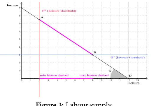
[image:20.612.92.353.343.523.2]At first sight, it might appear that, because our model is lexicographic (unlike mod-els with reference dependence and targeting, which have weights and trade-offs), the behaviour of the agent is entirely determined by the priority accorded to the two types of properties. For example one may suppose that agents giving priority to income react to drops in wages by increasingtheir labour supply, a negative elasticity that as explained is implausible in the textbook model. But in fact our model has a richer and more nuanced set of implications. The reason is simple. There is a qualitative differ-ence between income properties and leisure properties. Foranyleisure property there always is a feasible leisure-income combination satisfying that property.
Figure 3:Labour supply
But, on the contrary, for any
income property there is always a sufficiently low wage such that there is no leisure-income com-bination satisfying that property. This is a general observation, about target properties: one can-not (if he is sane) be ‘unrealis-tic’ with an objective constraint -like hours in a day-, but one can be unrealistic with a subjec-tive constraint -like how much one thinks his work is worth. Because of this asymmetry, de-pending on the realisation of the wage even a state giving in principle priority to a target income will simply force the agent to move on to consider the next property, something that will never occur for leisure properties. Consider the situation in fig-ure 3, depicting choices at some given wagew. The income and the leisure property,
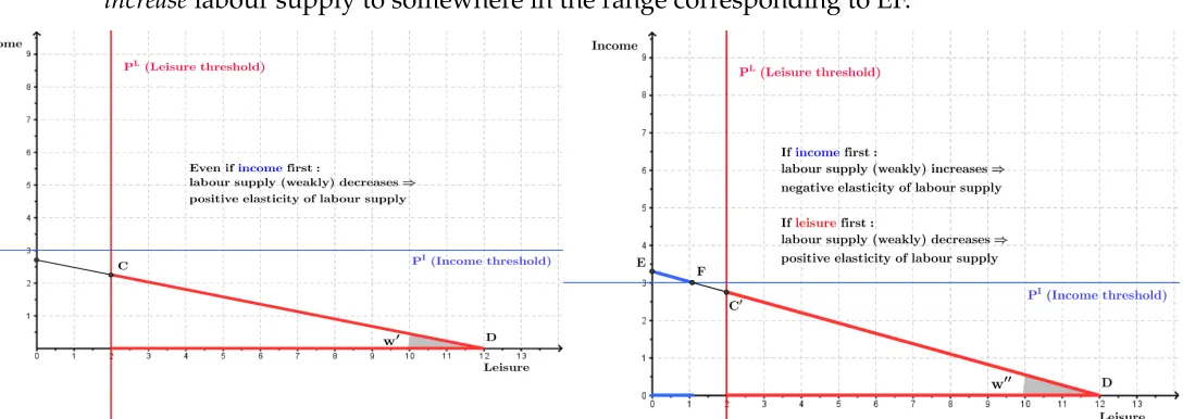
w0 <w, as illustrated in figure 4.
Once again, the state is irrelevant: the same set of acceptable alternatives CD is determined independently of the order, since if the income propertyPI is applied first it will not have any bite. The set of acceptable choices does not contain any choice with lower leisure than the acceptable choices at the higher wage w, and contains many choices with higher leisure. This is broadly consistent with the effect predicted by the textbook model and with the empirical evidence analysed in Farber [21].
However, the state becomes crucial in determining the agent response to a milder drop in wage, tow00with w0 < w00 <w, as depicted in figure 5. Here it is still possible that the regular comparative statics result holds, if PL is applied first. Yet if the agent is an ‘income type’ and instead appliesPI first, his response to the drop in wage is to
[image:21.612.44.588.294.487.2]increaselabour supply to somewhere in the range corresponding to EF.
Figure 4: Labour supply and a large drop in wage Figure 5:Labour supply with a modest drop in wage Furthermore, regardless of whetherPLorPI is applied first, our model predicts that
labour supply will never range in the values corresponding to leisure levels identified by the FC’ range in figure 5 - any contrary observation would falsify our model, and the higher the leisure or wage threshold levels (i.e. the farther to the northeast the intersection between the two threshold properties moves), the larger the labour supply ‘gap’.
Thus, the mechanism we have studied is consistent with textbook labour supply responses to large wage changes, but also allows a wider range of responses to milder wage changes, including negative wage elasticities. Negative wage elasticities are pre-dicted when the agent targets income before leisure.
of KR’s reference dependent model, which also accommodates both types of effects. In CM/KR, there is an element of rational expectations in that the reference targets are determined endogenously and ‘correctly’ by the agent, but the anomalous supply response can only occur for unanticipated wage changes. In our mechanism, on the contrary,targets are exogenous unobserved variablesbecause they are very much like pref-erences in standard theory, that is fundamental primitives and not an additional vari-able in a utility framework. Thus, they are not necessarily rationally determined: but, on the other hand, the anomalous responses can occur for perfectly predicted wages without requiring expectation errors as in the reference dependence model.
In summary, then, our analysis points to two novel implications. First, the size
of the wage change is a potentially important factor in the contrasting empirical ev-idence. Second, if state dependence explains labour supply then this supply can be ‘behaviourally extreme’, that is, for certain values of the wage there is a range of inter-mediate values of supply that are never chosen in any state: the worker either demands ‘a lot’ or ‘little’ labour, depending on the state. These hypotheses seem to merit further study both empirically and theoretically.
Of course, the above is just a sketch of a complete model, but it is precisely its sim-plicity coupled with the richness of implications that suggests its potential usefulness in more detailed frameworks. Similar applications of the theory can be made for exam-ple to saving decisions (along the lines of the examexam-ple in section 3.1, explaining why visceral immediate consumption impulses may become more relevant at low rates of return on savings and why savers may be subject to behavioural swings); or to con-sumer theory (explaining the behaviour of a ‘consumption-target driven’ concon-sumer).
6
Related literature
6.1
Multiself models
choice observation.16
To understand the puzzle, since in the KRS model for any A we can simply pick a preference that puts the choice from Ain the highest indifference class in A, it may happen that x is strictly preferred to yin A, but it is indifferent toy in another menu
B when two different preferences are applied to A and B. Therefore it may happen that xis chosen and yis rejected from A, while both x and yare chosen from B, thus violating Togetherness. This highlights the centrality in our model of thefixed nature of the mindset. The fact that departures from ‘rationality’ in choice can only be attributed to state dependence, and not to the mindset, imposes, unlike the KRS model, some discipline on behaviour.
Similar observations hold for the recent works by Green and Hojman [24] and Am-brus and Rozen [3]. Green and Hojman describe an agent as a probability distribution over all possible preference orderings. Such preferences are then aggregated via a vot-ing rule. If the votvot-ing rule satisfies a certain monotonicity property, this model can also explain any choice behaviour. Ambrus and Rozen study a very general model of a decision maker as a collection of utility functions (‘selves’), which encompasses many other models in this vein. Each menu may activate a different aggregation procedure of the various selves. This aggregation procedure is constrained to satisfy some natural axioms, which however force the aggregation rule to incorporate some cardinal infor-mation: this contrasts with our and the other models mentioned in this section, which are purely ordinal. Ambrus and Rozen’s central result is that with a sufficient number of selves any choice observation can be explained, in spite of the restrictions imposed on the aggregation procedure. This result suggests that multiselves models need to limit the number of allowable selves in order to exhibit observable restrictions. Re-placing ‘selves’ with ‘states’, this intuition could also apply to our framework. Because our analysis specifies the components of a state, one obvious way to restrict a state is to limit the number of properties that constitute it (some environments may specify natural restrictions). We also have noted above how the assumption of nestedness of the states makes our model equivalent to utility maximisation.
16To be precise, KRS deal with choice functions. We are referring to the obvious extension of their
6.2
Choice with frames
As observed in section 4, the choice functionsγ(.,<m) when single-valued can be
in-terpreted as choice with frames (Salant and Rubinstein [53]), where each state<mplays
the role of a specific frame. Of course, in our framework a checklist is a very different object from a utility function, as a linear order of a fixed set ofpropertiesrather than of alternatives. However using Proposition 1 as a bridging result, we can associate with each<m a weak order on the set of alternatives. When the weak order is a strict linear
order, such a substitution generates a choice function that Salant and Rubinstein term ‘choice by salient consideration’ (a single-valued choice function that maximises some frame dependent strict linear order on the alternatives). In the proof of Proposition 6 however we implicitly prove that acwith a environmental checklist can always be seen (in our domain) as the union of single-valued choice functions. In short, then, we can establish an observational equivalence between the choice correspondence induced by a choice by salient consideration as frames vary, and the choice correspondencec in-duced by γ(.,<m) as states vary. The upshot is that, as a by-product, Proposition
6 also provides a characterisation (hitherto not available) of choice correspondences generated by salient consideration choice functions.
The fact remains, however, that it might not be possible to identify the set of frames needed to interpret an observed choice as framed with the states that generated it. For an extreme example, ifxandyhave the same properties and there is asinglestate, we still need at least twoframes to generate, for example, the choice c({x,y}) = {x,y}. This discrepancy would not go away even if we extended the frame model to allow for multivalued choices in each state, for reasons similar to those explaining the discrep-ancy between menu dependent utility maximisation and menu driven state dependent choice. For example, ifx andy are as above, they will always appear together in any choice (since they must be ‘indifferent’ in any state), but one could instead define a frame in which xis ranked above y. So, at the conceptual level, the state dependence model remains distinct from the frame model. If states or frames could be observed, or if at least the choices corresponding to each state/frame could be observed, the two models could be easily told apart.
[42] model of choice by lexicographic semiorder) the correspondence would be lost.
6.3
Distinguishing state dependent from indecisive behaviour
Distinguishing between thepsychological reasonsthat motivate behaviour is important in many economic contexts. In this section we compare state dependence with an important psychological driver, indecisiveness (Eliaz and Ok [18], Mandler [39]). In-decisiveness is conceived by Eliaz and Ok and Mandler as the lack of either a strict preference or an indifference.
A simple property characterises the choice behaviour of indecisive agents in Eliaz and Ok’s [18] model:
WARNI (Weak Axiom of Revealed Non-Inferiority): If in a menuAthere is an alter-nativexthat is chosen, possibly from different menus, in the presence of each alterna-tive inA, then xshould be chosen fromA. Formally, for all A,B∈ Σ:
[∀y∈ A∃B∈ Σsuch thatx ∈ c(B), y∈ B]⇒ x∈ c(A).
Eliaz and Ok assume that the agent maximises an incomplete preference relation, and thus interpret the fact thatx ∈ c(B)andy ∈ Bas revealing the non-inferiority ofx
compared toy(though not necessarily its superiority). This suits a situation in which an agent is undecided, rather than indifferent, between two alternatives (in which case he cannot rank them). It is easy to see that both our models of state dependent be-haviour have different empirical predictions from Eliaz and Ok’s model of indecisive-ness. Call acthat satisfies WARNI but not WARP anindecisive choice.
Claim 2 There are (multivalued) menu driven state dependent choices that are not indeci-sive,17 and vice-versa. Similarly, there are (multivalued) environment driven state dependent choices that are not indecisive, and vice-versa.
Other comparisons that it would be interesting to make are with the psychological phenomena ofinattention(Masatlioglu et al. [46]),categorisation(Manzini and Mariotti [43]) and rationalisation (Cherepanov et al. [11]). However, all these theories, while axiomatised, are formulated for single-valued choices, whereas ours is crucially pred-icated on multiple observations of choice from menus. Therefore, pending a gener-alisation of those theories to choice correspondences, only the following basic claim can be made: there are menu driven state dependent choices that cannot be explained
by inattention, categorisation or inattention, and not viceversa (menu driven state de-pendent choice is unrestrictive when single-valued) and there are choices driven by inattention, categorisation and rationalisation that are not environment driven state dependent choices, and not viceversa (sd-WARP reduces to WARP in the single-valued case).
7
Concluding remarks
In this paper we have proposed a versatile framework to study the dependence of choices on psychological states. The language of properties we have adopted allows one to talk about such states in a more nuanced way, and with more direct psycho-logical interpretations, than the language of utility. The framework can accommodate much non-standard behaviour, yet we have shown that it is not empirically vacuous.
‘Psychological’ theories of choice that use primitives different from a standard util-ity function face a potential problem: namely, that it’s hard to tell precisely how dif-ferent they are from the textbook model.18 While this problem may be legitimately addressed in various ways, we have found it useful to address it through anaxiomatic
characterisation. In this way we have (a) pinned down the precise regularities in choice behaviour implied by the state swings of our framework - generating testable impli-cations on choice data - and (b) located our models in the ‘logical space’ of standard revealed preference axioms, facilitating comparison both with the textbook model and with other psychological theories of choice. Our models are, in a sense made precise, ‘between’ the standard model and certain weakened versions of it. In addition, the models are tractable: with appropriate restrictions, a rich set of specific economic im-plications can be derived.
In both models we have considered, the idea at the heart of their testability and distinctiveness is that an observer can garner data on multiple choices from the same menu (with single-valued observations, our first model would be empirically vacu-ous and our second model would reduce to the standard utility maximisation model). These multiple observations of choice from a menu can be taken literally, as for a con-sumer observed to pick different items from a shelf in different shopping days, taxi drivers choosing different hours of work in different days at the same daily wage, or experimental subjects approving multiple options. We hope that our results will spur
18See e.g. Gul and Pesendorfer [25] for a surprising application of the revealed preference method to
the collection of this type of data. But multiple observations of choice can also be interpreted as deriving from a (possibly estimated)stochastic choice function. In this case, the choosable alternatives inc(A)can be interpreted for example as all those al-ternatives that are chosen with positive probability, or as those that are chosen with maximum probability, or any of the intermediate possibilities. Then, depending on the specific connection made between deterministic and stochastic choice function, our characterisation results for the deterministic model will translate into different restric-tions on the probabilistic one.19 Obviously, the data needed to test our theory are less demanding than the collection of stochastic choice data - we just need to tellwhetheran alternative is choosable, without worrying about the precise frequency -, yet even the latter can be collected without too much difficulty (see e.g. Caplin and Dean [9] for a recent design that even elicits state-dependent stochastic choices).
In practice, a state is not entirely unpredictable: psychological research may help to identify correlations between environmental and personal variables with states, and states with choice, so that additional elements of predictability in choice can be identi-fied. For example, in the taxi driver application of section 5.1, one might conjecture a relationship between weather and psychological state, so that weather could be used as an observable proxy for states (or, conversely, one could use choice data toinfer a connection between choice and state, conditional on the theory being valid). Our con-tribution has been to identify what can be predictedexclusivelyin terms of an economic choice model.
While a psychological state affects choice, undoubtedly choice affects the psycho-logical state, too. There is a subtle two-way interaction between psychopsycho-logical states and choices. At present it is not clear how this interaction can be modelled, yet some progress has been made.20 Our paper is a first step towards the formal modelling of state dependent choice behaviour.
19A classical technical treatment of the relationship between deterministic choice correspondences
and stochastic choice functions is Fishburn [23].
20See for example, Dalton and Ghosal [13], who resolve the interaction through an elegant equilibrium
References
[1] Aizerman, M.A. and Fuad Aleskerov (1995),Theory of choice, North Holland, Am-sterdam and New York.
[2] Aizerman, M.A. and A.V. Malishevski (1981) “General theory of best variants choice: some aspects”,IEEE Transactions on Automatic Control, 26:1030–40.
[3] Ambrus, A. and K. Rozen (2013) “Rationalizing Choice with Multi-Self Models”, forthcoming in theEconomic Journal.
[4] Apesteguia, J. and M. A. Ballester (2013) “Choice by Sequential Procedures”,
Games and Economic Behavior, 77 (1): 90–99.
[5] Bernheim, B. D. and A. Rangel (2009) “Beyond Revealed Preference: Choice-Theoretic Foundations for Behavioral Welfare Economics”, Quarterly Journal of Economics, 124:51-104.
[6] Berry, S., J. Levinsohn and A. Pakes (1995) “Automobile Prices in Market Equilib-rium”,Econometrica63(4): 841-90.
[7] Camerer, C., L. Babcock, G. Loewenstein and R. Thaler (1997) “Labor Supply of New York City Cabdrivers: One Day at a Time”, Quarterly Journal of Economics, 112: 407–41.
[8] Caplin, A. and J. Leahy (2001) “Psychological expected utility theory and antici-patory feelings”,Quarterly Journal of Economics, 116: 55-79.
[9] Caplin, A and M. Dean (2013) “Rational Inattention and State Dependent Stochas-tic Choice”, mimeo, NYU.
[10] Capra, C. Monica (2004) “Mood-driven behavior in strategic Interactions”, Amer-ican Economic Review Paper and Proceedings94(2): 367-372.
[11] Cherepanov, V., T. Feddersen and A. Sandroni (2013) “Rationalization”,Theoretical Economics, 8 (3): 775–800.
[12] Crawford, V. P. and J. Meng (2011) “New York City cab drivers’ labor supply revis-ited: reference-dependent preferences with rational-expectations targets for hours and income”,American Economic Review101: 1912–1932.
[13] Dalton, P. and S. Ghosal (2008) “Behavioral decisions and welfare”, Warwick Eco-nomic Research papers n. 834, University of Warwick.
[14] Dekel, E., B. Lipman and A. Rustichini (2001) ”Representing Preferences with a Unique Subjective State Space,”Econometrica69: 891-934.
[15] Dietrich, F. and C. List (2013) “Reason Based Rationalization”, mimeo, London School of Economics.
http://economics.sas.upenn.edu/˜ddill/DillenbergerRozen HDRA%20FEB2013.pdf. [17] Ehlers, L. and Y. Sprumont (2008) “Weakened WARP and top-cycle choice rules”,
Journal of Mathematical Economics44 (1) 87-94.
[18] Eliaz, K. and E. Ok. (2006) “Indifference or indecisiveness? Choice theoretic foun-dations of incomplete preferences”,Games and Economic Behavior56: 61–86.
[19] Erber, R., M. Wang and J. Poe (2004). Mood regulation and decision making: Is irrational exuberance really a problem? In I. Brocas and J.D. Carrillo (eds.), ‘The psychology of economic decisions’ (II:197-210), Oxford University Press.
[20] Ergin, H. and T. Sarver (2010) “A Unique Costly Contemplation Representation”,
Econometrica78: 1285-1339.
[21] Farber, H.S. (2005) “Is tomorrow another day? The labor supply of New York City cabdrivers”,Journal of Political Economy, 113: 46-82.
[22] Farber, H.S. (2008) “Reference-dependent preferences and labor supply: the case of New York City taxi drivers”,American Economic Review, 98: 1069–82.
[23] Fishburn, P.J. (1978) “Choice probabilities and choice functions”,Journal of Mathe-matical Psychology18: 205-19.
[24] Green, J. and D. Hojman (2008) “Choice, rationality and welfare measurement”, mimeo, Harvard IEResearch Discussion Paper n.2144.
[25] Gul, F. and W. Pesendorfer (2005) “The Revealed Preference Implications of Ref-erence Dependent PrefRef-erences”, mimeo, Princeton University.
[26] Ifcher, J. and H.S. Zarghamee (2011) “Happiness and time preference: the effect of positive affect in a random-assignment experiment”, American Economic Review, 101(7): 3109-29.
[27] Isen, A.M. (2000) ‘Positive affect and decision making’, In M. Lewis & J.M. Havieland (eds.),Handbook of emotions(2:417-35). London: Guilford.
[28] Kahn, B.E., and A.M. Isen (1993) ‘The influence of positive affect on variety seek-ing among safe, enjoyable products’,Journal of Consumer Research, 20:257-70. [29] Kalai, G., A. Rubinstein and R. Spiegler (2002) “Rationalizing choice functions by
multiple rationales”Econometrica, 70: 2481-2488.
[30] Kirchsteiger, G., L. Rigotti and A. Rustichini (2006), “Your morals might be your moods”,Journal of Economic Behavior & Organization, 59:155-72.
[31] Kliger, D. and Levy, O. (2003) “Mood-induced variation in risk preferences”, Jour-nal of Economic Behavior & Organization, 52:573-84.
[32] K ¨oszegi, B. (2010) “Utility from anticipation and personal equilibrium”,Economic Theory, 44:415-44.
[33] K ¨oszegi, B. and M. Rabin (2006) “A model of reference-dependent preferences”,
[34] Kreps, D. M. (1979) “A Representation Theorem for ‘Preference for Flexibility’ ”,
Econometrica, 47: 565-577.
[35] Laibson, D. (2001) “A cue-theory of consumption”,Quarterly Journal of Economics, 116:81-119.
[36] Lancaster, K. J. (1966) “A new approach to consumer theory ”,The Journal of Polit-ical Economy, 74 (2): 132-157.
[37] Litvakov, B.M. (1981) “Minimal representation of joint-extremal choice of op-tions”, Automation and Remote Control 1: 182-184.
[38] Mayer, J., Y. Gaschke, D. Braverman and T. Evans (1992) “Mood-congruent judg-ment is a general effect”,Journal of Personality and Social Psychology, 63: 119-132. [39] Mandler, M. (2009) “Indifference and Incompleteness distinguished by rational
trade”,Games and Economic Behavior67:300-14.
[40] Mandler, M., P. Manzini and M. Mariotti (2012) “A million answers to twenty questions: choosing by checklist”,Journal of Economic Theory, 147:71–92.
[41] Manzini, P. and M. Mariotti (2007) “Sequentially rationalizable choice”,American Economic Review, 97:1824-39.
[42] Manzini, P. and M. Mariotti (2012) “Choice by lexicographic semiorders”, Theoret-ical Economics, 7: 1-23.
[43] Manzini, P. and M. Mariotti (2012) “Categorize then choose: boundedly rational choice and welfare”,Journal of the European Economics Association, 10: 1141–65. [44] Manzini, P. and M. Mariotti (2013) “Stochastic choice and consideration sets”,
Econometrica, 89(3): 1153-1176.
[45] Manzini, P., M. Mariotti and C.J. Tyson (2012) “Two-stage threshold representa-tions”,Theoretical Economics, 8 (3): 875–882.
[46] Masatlioglu, Y., D. Nakajima and E. Ozbay (2012) “Revealed attention”,American Economic Review102:2183–205.
[47] Mittal, V., and W.T. Ross (1998) “The impact of positive and negative affect and issue framing on issue interpretation and risk taking”,Organizational Behavior and Human Decision Processes, 76: 298-324.
[48] Nygren, T.E. (1998) “Reacting to perceived high- and low-risk win-lose opportu-nities in a risky decision-making task: is it framing or affect or both?”,Motivation and Emotion, 22:73-98.
[49] Nygren, T.E., A.M. Isen, P.J. Taylor, and J. Dulin (1996) “The influence of positive affect on the decision rule in risk situations: Focus on outcome (and especially avoidance of loss) rather than probability”,Organizational Behavior and Human De-cision Processes, 66: 59-72.
n. 4645.
[51] Rick, S. and G. Loewenstein (2008) “The role of emotion in economic behav-ior”, ch. 9 in The Handbook of Emotion, 3rd ed, M. Lewis, J. Haviland-Jones and L. Feldman-Barrett (Eds.), New York, Guilford.
[52] Rubinstein, A. and Y. Salant (2012) “Eliciting welfare preferences from behavioral datasets”,Review of Economic Studies, 79 (1): 375-387.
[53] Salant, Y. and A. Rubinstein (2008) “(A, f):Choice with frames”,Review of Economic Studies, 75: 1287–96.
[54] Thayer, R.E. (2000) ‘Mood’.Encyclopedia of Psychology, Washington, D.C.: Oxford University Press and American Psychological Association.
[55] Thayer, R.E. (2001) ‘Calm energy: how people regulate mood with food and exer-cise’, New York, Oxford University Press.
Appendices
A
Proofs
Proof of Proposition 2. We show the following: let c and d be two choice functions on Σ that have, respectively the sd-cheklists Γ,{<A}A∈Σ and
Γ,<0A A∈Σ; then
c =d.
Suppose thatc(A) 6=d(A)for someA∈ Σand in particular let (possibly relabeling the choice functions)x ∈ c(A)andx ∈/ d(A). The latter implies that there existy ∈ A
andP ∈ Γsuch thatx ∈/ Pand y∈ P. For x ∈ c(A)it must then be the case that there exists Q <A Pand z ∈ A such that y ∈/ Q and z ∈ Q. If P ⊂ Qthis is incompatible with y ∈ P, and if Q ⊂ P then x ∈/ Q. Therefore x ∈/ SA(Q,<A) and x ∈/ c(A), a
contradiction.
So any sequence of the properties in the mindset Γ generates the same behaviour and by Proposition 1 the behaviour generated by any particular sequence maximises a weak order, as claimed.
Proof of Proposition 3. Suppose thatc satisfies Togetherness. Define a relation ≈on
Xby x ≈yiff there is no A ∈ Σsuch thatx ∈ c(A)andy ∈ A\c(A)ory ∈ c(A)and
x ∈ A\c(A). The relation≈is obviously reflexive and symmetric. To see that it is also transitive, suppose thatx ≈ y ≈ zand that x ∈ c(A)and z ∈ Afor some A ∈ Σ. We show thatz∈ c(A).
Sincex ≈ywe havex ∈c({x,y,z})if and only ify ∈c({x,y,z})({x,y,z}is in the domain by assumption), and similarlyy ≈ zimplies that y ∈ c({x,y,z})if and only if z ∈ c({x,y,z}). Therefore if x ∈ c({x,y,z}) then c({x,y,z}) = {x,y,z}. There-fore by Togetherness x ∈ c(A) and z ∈ A imply z ∈ A. If instead x ∈/ c({x,y,z}), then c({x,y,z}) = ∅, a contradiction. ≈ is therefore an equivalence relation and
it partitions the set of alternatives into equivalence classes, which we denote [x] = {y∈ X : y≈ x}.
Given A ∈ Σ, take any x ∈ c(A) and let PA = [x]. Note that PA is uniquely
defined, and let the mindset beΓ= {PA : A∈ Σ}. Since≈is an equivalence, we have PA∩PB = ∅for all distinct menus A,B ∈ Σ. Let the state <A be any linear order for
whichPA <A Pfor all P ∈ Γ\PA. ThenA∩PA = c(A) (for anyy ∈/ c(A)and x ∈ PA