Pairwise interaction point processes for modelling bivariate spatial point patterns in the presence of interaction uncertainty

September 2015, Volume 7, Issue 3. http://www.jenvstat.org

Pairwise Interaction Point Processes for Modelling

Bivariate Spatial Point Patterns in the Presence of

Interaction Uncertainty

Glenna F. Nightingale1_{, Janine B. Illian}2_{, and Ruth King}3 [email protected], [email protected], [email protected]

1_{School of Geography and Geosciences}

2_{School of Maths & Statistics and Centre for Ecology and Envrionmental Research}

University of St. Andrews, Scotland, KY16 9LZ, U.K. 3_{School of Mathematics, University of Edinburgh,}

James Clerk Maxwell Building, The Kings Buildings, Peter Guthrie Tait Road, Edinburgh, EH9 3FD, U.K.

Abstract

Current ecological research seeks to understand the mechanisms that sustain biodiver-sity and allow a large number of species to coexist. Coexistence concerns inter-individual interactions. Consequently, there is an interest in identifying and quantifying interactions within and between species as reflected in the spatial pattern formed by the individuals. This study analyses the spatial pattern formed by the locations of plants in a commu-nity with high biodiversity from Western Australia. We fit a pairwise interaction Gibbs marked point process to the data using a Bayesian approach and quantify the inhibitory interactions within and between the two species. We quantitively discriminate between competing models corresponding to different inter-specific and intraspecific interactions via posterior model probabilities. The analysis provides evidence that the intraspecific interactions for the two species of the genusBanksiaare generally similar to those between the two species providing some evidence for mechanisms that sustain biodiversity.

1. Introduction

1.1. Modelling Biodiverse Plant Communities

Mechanisms or biological processes which maintain biodiversity and hence facilitate the co-existence of a large number of species have been the focus of numerous ecological studies (Grinnell 1917;Janzen 1970; Hubbell 1997;Siepielski and McPeek 2002;Wright 2002; Mur-rell and Law 2003;Zillio and Condit 2007). Consequently, an understanding of such processes is of central importance to biodiveristy preservation.

Modelling species interactions in a spatial context involves analysing the spatial pattern formed by individuals in ecological communities to reveal the individuals’ local interactions and hence to inform on the interaction structure in a community (Murrell and Law 2003). A spatial point pattern therefore can be considered as a spatial signature, which, if decoded, can shed light on the interactions among and within the species in a plant community. A growing number of publications has focused on the analysis of these spatial point patterns both based on descriptive statistics (Liebhold and Gurevitch 2002;Wiegand and Moloney 2004; Comas and Mateu 2007) and on point process models (Thompson 1955;Gatrellet al.1996;Khaemba 2001).

Spatial point process models describe the overall properties of spatial patterns, while taking every individual in a community into account (Illian et al. 2008). Both in the ecological and in the statistical literature, most studies using spatial point processes, model the pattern formed by a single species only (Illian et al. 2012; Ewel and Hiremath 2006; Møller and Waagepetersen 2003; Diggle 2003; Callaway 1995). So far, few studies involve multivariate patterns i.e. patterns formed by two or more species (Baddeley and Turner 2000; Wiegand et al.2007;Illianet al.2009;Picardet al.2009). However, in models of multi-species patterns the number of ”intra-”, and ”inter-” specific interactions and hence the number of interaction parameters grows with the number of species. Hence suitable methods for model selection are required to compare different models and to avoid over-parameterization. In this analysis we consider a two species (bivariate) dataset comprising of species of the same genus.

1.2. The Dataset

The dataset comprises of two species of the genus Banksia, from a 22×22 metre plot from Cataby, Western Australia (Armstrong 1991). The two species have been classified as re-sprouters, which exhibit a particular fire regeneration strategy. Resprouters regenerate from root stocks after a fire (Bell 2001). Due to low nutrient levels in the sandy soil that char-acterize the study area, resprouters reproduce very slowly but the existing individual plants are likely to have existed in the same location for a very long time (Armstrong 1991; Illian et al. 2009). Overall, environmental conditions, in particular the nutrient and water levels in the soil may be considered homogeneous within the plot (Armstrong 1991; Illian et al. 2009). As a result of the homogeneity of the soil conditions, this dataset allows us to model interactions within a plant community without the need to include environmental spatially explicit covariates that potentially impact on the pattern.

methods to discriminate between competing models in terms of the interactions present within and between species (or intra- and inter-specific interactions respectively). Figure1illustrates the bivariate point pattern formed by the two resprouter species in this study.

[Figure 1 about here.]

1.3. Exploratory analysis

An exploratory analysis of the data was conducted using the L-function Besag (1977) and the pair correlation function (Diggle 1983;Baddeleyet al. 2007;Stoyan and Penttinen 2000; Illianet al.2008;Lawet al. 2009) .

L-function

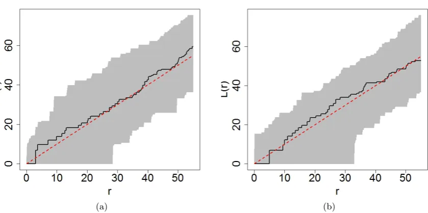
The L-function was introduced byBesag(1977), and is strongly related to Ripley’s K function. This function is commonly expressed as L(r), where r denotes the interaction radius, may be used to assess point patterns for complete spatial randomness. Typically, the empirical L-function is compared to that obtained for a point pattern derived from Poisson point process (theoretical L-function). The value of the theoretical L-function is equal tor for a stationary Poisson process at all distances. In this analysis, the L-function was plotted for each species, each with a corresponding simulation envelope obtained from 10,000 instances (Figure2) of a Poisson point process.

[Figure 2 about here.]

In each plot, the theoretical L-function is denoted by a dotted red line and the empirical L-function by a solid black curve. If the curve obtained for the empirical L-function was above/below the simulation envelope, this could indicate the possibility of clustering/regularity beyond that expected under conditions of complete spatial randomness (CSR). The inclusion of simulation envelopes around the line for the theoretical L-function gives us an indication of how much deviation is associated with the realisations.

In general, the curve for the empirical L-function for Banksia menziesii fluctuates above and below the reference line representing the theoretical L-function. Despite this, the curve remains within the simulation envelopes. For Banksia attenuata, the curve for the empir-ical L-function is observed to be predominantly above the line representing the theoretempir-ical L-function, this however remains within the simulation envelopes. Overall, we note that both plots fall within the respective simulation envelopes thus providing no evidence against complete spatial randomness at the exploratory level.

Pair correlation function

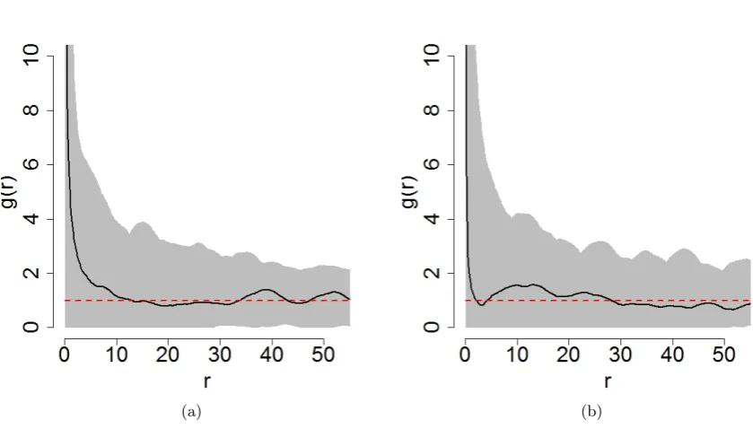
The pair correlation function, commonly expressed asg(r), is also useful in providing a spatial summary of a given point pattern. Specifically,g(r) provides an indication of the dependency of points at a given distance r for a given point pattern. This function is a derivative of Ripley’s K function and is expressed as

g(r) = K 0_(r)

For point pattern which exhibits CSR, g(r) = 1 for all values of r. If g(r)> r this suggests that there is spatial dependency between the points. That is, the interpoint distancer occurs more frequently than under conditions of CSR. The converse is true forg(r)<1. Ifg(r) = 0, this suggests that there are no points within the specified interpoint distancer. In this caser is termed a ‘hard core radius’. The pair correlation function was plotted for both species and is shown in Figure3with simulation envelopes obtained from 10,000 replications of a Poisson point process.

[Figure 3 about here.]

From Figure 3 it is clear that for each species, the corresponding empirical plot fluctuates above and below the reference line, but remains within the simulation envelopes. This suggests that there is no evidence against CSR.

These summary characteristics only provide preliminary results and are limited in that each analysis only assess the behaviour of a single species in the study area. A more formal approach would include point process models which provide estimates of the interactions between species. We focus on these models in the next section.

2. Method

2.1. Gibbs processes, specific model choice

Gibbs processes are point processes which model patterns exhibiting inhibition or aggregation, i.e. interaction among the points (Illianet al.2008). We consider a pairwise-interaction Gibbs process (Baddeley and Turner 2000) to model a bivariate point pattern. In particular, we let the points in a given point pattern x, contained in a bounded region in spaceW, represent objects of interest such as plants. If each point is accompanied by additional information (such as which species it represents) the point pattern is a marked point pattern (Illianet al. 2008). Each point is associated with a mark m ∈ M where M is the mark space. In our example we let the marks denote the different species of interest so thatM ={1,2}.

A Gibbs process is characterized by a set of intensity and interaction parameters. The intensity parameters, are denoted by β1 and β2 and represent the intensity of plants per unit area (1dm2) from species 1 and species 2, respectively. The full parameter set for the Gibbs process used here is denoted byθ={β1, β2, γ11, γ22, γ12}.

In general, pairwise interaction processes are suitable for modelling regular point patterns, whereas area interaction point processes are appropriate for modelling aggregated point pat-terns (King et al. 2012). In the pairwise interaction process we consider here, interactions within or between species groups are negative interactions and are inhibitory in nature. The interaction parameters take values within the range of 0 to 1 where lower values indicate a higher degree of inhibition. In the special case where the interaction parameter is 0 there is hard core inhibition such that there is a circle of fixed interaction radius around each plant within which no other plant is found. Conversely, an interaction parameter of 1 corresponds to no interaction resulting in complete spatial randomness.

Let n1 and n2 denote the number of individuals in species 1 and 2 respectively, and set

υ1 = {υ11, . . . , υ1n1} and υ2 ={υ21, . . . , υ2n2} where υij denotes the j

For notational convenience the full set of data is denoted byυ ={υ1,υ2}.

To specify the interaction function we follow Illian et al.(2009). For the two point patterns

υ1 and υ2 we express the interaction functions(υ1|υ2) as

s(υ1|υ2) = n1 X i=1 n2 X j=1

h(kυ1i−υ2jk), (1)

wherekυ1i−υ2jkrepresents the Euclidean distance betweenυ1i andυ2j. We expresshin the

form:

h(r) =

(1−(r/R)2)2 if 0< r≤R

0 otherwise,

where R is a fixed interaction radius as mentioned earlier. We note that for this interaction function, the magnitude of the interaction between plants is not considered to be constant as for example in a Strauss process, but to decrease with increasing distance (up to a fixed distance R).

The interaction parameters γ11, γ22 and γ12 represent the interaction within conspecifics of species 1, within conspecifics of species 2 and between individuals from species 1 and 2, respectively.

The corresponding pseudolikelihood of the data can be expressed as a function of the intensity parameters β = {β1, β2} and the interaction parameters γ = {γ11, γ22, γ12} (Baddeley and Turner 2000). In particular we have,

f(υ;θ) =αβn1

1 β

n2

2 γ

s(υ1|υ1)

11 γ

s(υ2|υ2)

22 γ

s(υ1|υ2)+s(υ2|υ1)

12 ,

where α is an intractable normalising constant given by

α= exp

−β1

Z

W

γ₁₁t(u,v1)γ₁₂t(u,v2)du−β2

Z

W

γ₁₂t(u,v1)γ₂₂t(u,v2)du

, (2)

for the function t defined below. Let u be an arbitrary point in the study region W. For

i= 1,2, we set

t(u,υi) = ni

X

k=1

h(ku−υikk). (3)

An approximation to this integral term can be obtained by using numerical integration tech-niques such as the Berman-Turner device (Baddeley and Turner 2000). This pseudolikelihood is expressed for the saturated model which contains all the possible interactions γ11, γ22 and

γ12. Submodels can be defined by different combinations of the presence or absence of these three interaction parameters. In total, for a bivariate point pattern, eight different models can be constructed corresponding to the inclusion or exclusion of each of the different interaction terms in the model.

Border edge correction was used in this analysis. Consequently, parameter estimation is based on a ‘reduced sample’ or subregion of W, such that all the points in the subregion are within at leastRunits from the boundary ofW. Note that the points which are withinR units from the boundary of W, or ‘edge points’, are still considered as possible ‘neighbours’ of points in the ‘reduced sample’. The reduced sample can be expressed as:

whereB(u, R) represents a disc of radiusR centered atu. R is chosen here to be equivalent in value to the chosen interaction radius.

The application of border edge correction results in estimating the pseudolikelihood described above using a modified interaction function. The interaction function described in Equation 1, is redefined such thats(υi|υj) is estimated by s(υ−i |υj) and the integral in Equation2 is

now expressed overWR instead ofW. As a result of the renewed specification of the domain

for this integral, the functiont, described in Equation 3is redefined such thatu∈WRrather

than the previous specification ofu∈W.

Various methods have been proposed for estimating the interaction radius used in point pro-cesses when relevant knowledge is not available. The consideration of the radius of interaction as a model parameter has been explored by Illian et al. (2008) and Berthelsen and Møller (2002). Illian et al. (2008) construct a hierarchical model of one group of species given the spatial location of a second species group. For this analysis a flat prior of N(0, σ2) restricted to [0,∞) is used for the interaction radii parameters. One challenge identified in this study is that for a highly biodiverse dataset, the high dimensionality of the set of interaction radii results in high computational costs. Alternatively, Berthelsen and Møller (2002) treat the interaction radius as a parameter where spatial birth and death processes are used for perfect simulation of univariate Gibbs point processes.

In other studies the interaction radius is derived from biological knowledge (King et al.2012; Illian and Hendrichsen 2010) and visual inspection of exploratory plots such as the plot of Ripley’s K function (Picardet al.2009). Kinget al.(2012) andIllian and Hendrichsen(2010) both model musk-oxen herds using different modelling approaches. Illian and Hendrichsen (2010) andMøller and Waagepetersen (2003) note that the interaction radius may be more formally estimated by using a profile likelihood approach.

For the dataset considered in this paper, the interaction radii specified are based on biological background information provided and cited byIllianet al.(2008). A range for the interaction radius for each of the species considered in this analysis is provided. The range for the interaction radius forB. attenuata is 1.5−4.0 m and that forB. menziesii is 0.5−2.5 m. We adopt an interaction radius of 2.5m for each species.

2.2. Bayesian Approach

We adopt a Bayesian approach for inference on the model parameters. The joint posterior distribution of the parameters is formed by combining the likelihood of the data with the corresponding prior distribution of the parameters. However, in our case we do not have an explicit likelihood function, but a pseudolikelihood. The use of the pseudolikelihood in a Bayesian context has been proposed by several authors including Efron (1993); Chang and Mukerjee (2006); Venturaet al. (2009).

For notational convenience we let the pseudolikelihood of the data given the parameters be denoted as f(υ|θ). The posterior distribution of the parameters can be written as:

π(θ|υ) ∝ f(υ|θ)p(θ),

(MCMC) algorithm. However due to the additional model uncertainty we extend the pos-terior distribution to incorporate this additional level of uncertainty. In particular, we treat the model itself as a discrete parameter and form the joint posterior distribution over both parameter and model space, given by,

π(θ, m|υ) ∝ fm(υ|θ)p(θ|m)p(m),

where θ defines the set of parameters in model m, fm(υ|θ) represents the pseudolikelihood

of the data given model m,p(θ|m) the prior distribution for the parameters in modelm and

p(m) the prior probability for model m.

To explore the posterior distribution and to obtain posterior summary statistics, we use a reversible jump (RJ) MCMC approach (Green 1995). This approach comprises two distinct steps.

Step 1. Update the parameters, conditional on the model, using the Metropolis Hastings algorithm.

Step 2. Update the model itself using a reversible jump step.

We consider only the second step in detail, since the Metropolis Hastings algorithm used in the first step is a standard random walk Metropolis update (Brooks 1998).

For the reversible jump step suppose that at iteration k, the Markov chain is in model m

with parameter vector θ so that the current model state is denoted as (θ, m). We initially propose to move to a new model, m0 where we choose each alternative model with equal probability. Given the proposed model we generate new parameter valuesθ0 ∼q(θ0) where q

is some proposal distribution function described in more detail below. We accept the move with probability min(1, A), where

A= π(θ

0_{, m}0_|υ)P(m|m0_)q(θ)

π(θ, m|υ)P(m0_|m)q(θ0₎

dθ0

dθ .

We note that the probabilities of moving from modelm to model m0, expressed as P(m0|m) and from model m0 to model m, expressed as P(m|m0), are equal (= 1₇) and cancel in the

acceptance probability. The final Jacobian term,

dθ0

dθ

, is simply equal to unity, so that the

acceptance probability termA, reduces to,

A= π(θ

0_{, m}0_|υ)q(θ)

π(θ, m|υ)q(θ0).

The final quantity to be defined in the updating step is the proposal density q. For this study, the proposal density q is a multivariate normal density function with mean (SD) and covariance matrix obtained from an initial pilot MCMC simulation for the given model. For further discussion of the MCMC reversible jump algorithm in ecological contexts see for example,Kinget al. (2009).

3. Results

3.1. Bayesian Analysis

et al. 2006) on the interaction parameters. In particular, we set logγ ∼ N(0, σ2) for γ =

γ11, γ12, γ22 where σ∼U[0,10].

We initially present the results for each individual model, before considering the issue of model selection. In each model the MCMC algorithm is run for 10,000 iterations with the first 1000 iterations discarded as burn-in. Running independent simulations from over-dispersed starting points produced essentially identical results and standard convergence diagnostics such as the BGR statistic (Brooks and Gelman 1998) suggested the chains had converged. The posterior summary statistics of the parameters in each individual model are given in Table1. The results also indicate that the intraspecific interaction for both species is relatively lower than that of the interspecific interaction. For example, in the saturated model, model 8, the posterior mean (SD) for the interspecific interaction is 0.028 (0.029) whereas that for the intraspecific interaction parameters are 0.591 (0.224) and 0.405 (0.182).

Overall, the posterior estimates obtained indicate that there is a negative relationship between the intensity parameters and the interaction parameters. This is to be expected, since smaller values of the interaction parameters correspond to increased inhibitions (either between or within species) which will typically result in an increased intensity to explain the observed point pattern and number of observed points (and vice versa). This negative correlation is clearly demonstrated in the posterior correlation between the intensity and associated inter-action parameters. For example, in the saturated model, the posterior correlation between intensity and intraspecific interaction in species 1 is −0.561 in the case of species 2, the posterior correlation is−0.471.

[Table 1 about here.]

We now consider the issue of model selection. The corresponding posterior model probabilities are also provided in Table 1. The model with the highest posterior probability corresponds to model 5, which contains one interaction parameter (γ12): the interaction between the two species. We note however that models 6 and 7 received similar posterior support (0.099, and 0.094). All models identified with non-negligible support contain the between species inter-action parameter,γ12indicating that the parameter and hence the interaction are important. The corresponding posterior probabilities for the presence ofγ11 and γ22 are similar, being equal to 0.117 and 0.112 or, equivalently, Bayes Factors (Kass and Raftery 1995) of 0.132 and 0.126, respectively (assuming all interactions are present) indicating a lack of posterior support for each within-species interaction.

In the saturated model, the posterior probability thatγ12 is less thanγ11 is 1; similarly, the posterior probability thatγ12 is less than γ22 is 1. Recall that lower values of the interaction parameter corresponds to a greater level of inhibition. This demonstrates the importance of the between species interaction within the model, and hence a high posterior model probability of being present. In the case of the intraspecific interaction estimates, the probability that

γ11 is greater than γ22 is 0.260, suggesting the level of within-species inhibition in species 2 is higher than that of species 1.

[Table 2 about here.]

a hierarchical prior on the variance of the interaction terms,σ2, and set σ ∼U[0,10]. Note that the estimation of this parameter is expected to be poor due to the very limited amount of information relating to this parameter. In addition, this parameter, σ, is present in all models except for model 1 (corresponding to the Poisson process). Thus, we would anticipate that changing the upper limit of the uniform prior would have limited impact on the posterior model probabilities within those models that contain an interaction (models 2-8). We consider the priorsσ∼U[0,1] andσ∼U[0,100], with the corresponding posterior model probabilities obtained given in Table2.

In our case, increasing the upper limit of the uniform prior on σ2 does not result in any significant changes in the posterior model probabilities. Placing a much lower value for the upper limit does have some impact on the posterior model probabilities, in the case that the limit begins to influence the posterior distribution forσ by constraining the values the parameter can take. For example, specifying aU[0,1] prior onσresults in a more constrained distribution forγ12. However, this prior would not be regarded as uninformative as it strongly influences the set of values the parameter can take due to its restrictive nature.

3.2. Interaction radius sensitivity

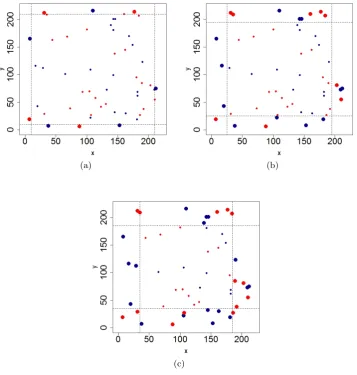
The interaction radii (or ‘zones of influence’) used for the species in this analysis are based on the ranges suggested by (Illian et al. 2009). The range for the interaction radius for B. attenuata is 1.5−4.0 m and that for B. menziesii is 0.5−2.5 m. We adopt an interaction radius sensitivity analysis using the same priors and interaction function described earlier. The additional interaction radii considered are 1.0, and 3.5 (recall previously that a radius of 2.5m was used). Figure4shows the reduced dataset (bivariate point pattern) after border edge correction has been applied for each of the radii considered.

[Figure 4 about here.]

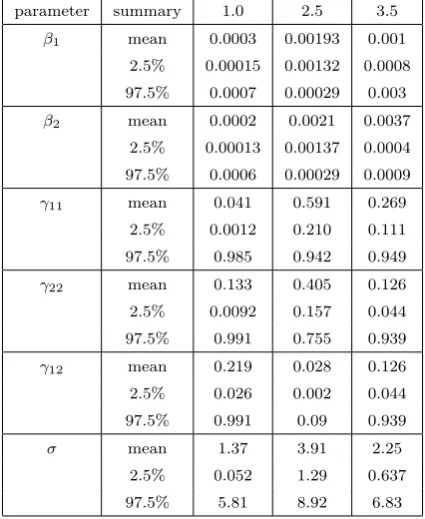
The results of the interaction radius sensitivity test are shown in Figure 3. The results indicate that as the interaction radius is increased, the posterior estimates for the interaction parameters increase in magnitude suggesting a decrease in the degree of inhibition between plants concerned. This is especially true for the intraspecific interaction parameters. Finally, the effect of the choice of interaction radius on model discrimination was also considered. The results indicate that the choice of interaction does affect the model which receives the highest posterior support. The posterior probabilities for the interspecific interaction parameter for radii 1.0, 2.5 and 3.5 are 0.040, 1.000, and 0.605 respectively.

[Table 3 about here.]

[Table 4 about here.]

4. Discussion

individuals forming the patterns. We have considered a Bayesian approach to analysing bivariate point patterns, with particular focus on model choice, i.e. on the assessment of the presence/absence of interactions present within the pattern. In particular, we obtain posterior model probabilities for the different competing models that quantitatively discriminate among the competing models and hence interactions present using a pilot-tuned reversible jump MCMC algorithm.

Biologically, the interactions are interpreted as competitive interactions where the magnitude of the interaction gives an indication of the ‘competitive strength’. In this analysis, we are able to not only quantify the presence/absence of the parameters for models where there is more than one interaction present, but also to obtain the relative strength of the interactions, by calculating the posterior probability that one interaction is greater than another. For our dataset, the intraspecific inhibitory interactions occurring in both resprouter species were found to be of similar strength. For the interaction between the two species there was strong evidence of the parameter representing this interaction should be included in the model.

Both species considered in this analysis are of the same genus, Banksia and hence possess similar biological characteristics. This is a possible explanation for the fact that the posterior estimates of the intraspecific interaction parameters were of similar magnitude. The posterior mean (SD) of the intraspecific interaction parameters for species 1 and 2 are 0.591 (0.224) and 0.405 (0.182), respectively, indicating that there is no evidence for a decisive character-isation of the nature of the intraspecific interaction. This is corroborated by the results of the exploratory analysis. With regard to the inter-specific interaction between the species, Richardson et al. (1995) describe the interaction between Banksia species as most strongly competitive (in comparison with the interaction between individuals of the Banksia species and other species) due to the fact that individuals of Banksia possess common features such as similar growth form and germination biology. Again, this is also evident in the results obtained. The value of the posterior estimate for the interspecific interaction parameter is comparatively much lower than that of the other interaction parameters. Individuals of two species exhibit proteoid or cluster roots, a feature common to all species of the genusBanksia. This root system involves masses of lateral roots giving rise to a dense horizontal root mat sys-tem. The inhibitory interaction between the two species could be due to competition between the species at the level of nutrient uptake by the root system. Connor and Bowers (1987) suggest that inter-specific competition gives rise to spatial signatures inherent in spatial point patterns.

Possible extensions to this approach in general include the use of covariates in the model, the consideration of asymmetric interactions between species and the use of area interaction point processes (Baddeley and Lieshout 1995; Comas and Mateu 2007). The inclusion of environmental covariates in the modelling process would lead to more complex point processes. Finally, the extension to multivariate point processes with more than two species is an area of active research where we consider novel approaches to circumventing the huge computational costs to modelling a highly diverse ecological communities.

References

Baddeley A, B´ar´any I, Schneider R (2007). “Spatial Point Processes and their Applications.” InStochastic Geometry, volume 1892 of Lecture Notes in Mathematics, pp. 1–75. Springer Berlin / Heidelberg.

Baddeley A, Lieshout M (1995). “Area Interaction Point Processes.” Annals of the Institute of Statistical Mathematics,47, 601–619.

Baddeley A, Turner R (2000). “Practical Maximum Pseudolikelihood for Spatial Point Pat-terns.”Australian and New Zealand Journal of Statistics,42, 283–322.

Bell DT (2001). “Ecological Response Syndrome in the Flora of Southwestern Western Aus-tralia: Fire Resprouters versus Reseeders.”The Botanical Review,67.

Berthelsen KK, Møller J (2002). “A primer on perfect simulation for spatial point processes.” Bulletin Brazilian Mathematical Society,33, 351–367.

Besag J (1977). “Contribution to the discussion of Dr.Ripley’s paper.”Royal Statistical Society B,39, 193–195.

Brooks SP (1998). “Markov Chain Monte Carlo Method and its Application.”The Statistician, 47, 69–100.

Brooks SP, Gelman A (1998). “General Methods for Monitoring Convergence of Iterative Convergence.”Journal of Computational and Graphical Statistics,7, 434–455.

Callaway RM (1995). “Positive Interactions Among Plants.” The Botanical Review, 61, 306–337.

Chang IH, Mukerjee R (2006). “Probability matching property of adjusted likelihoods.” Statist. Probab. Lett.,76, 838–842.

Comas C, Mateu J (2007). “Modelling Forest Dynamics: A Perspective from Point Process Methods.”Biometrical Journal,49, 176 – 196.

Connor EF, Bowers MA (1987). “The Spatial Consequences of Interspecific Competition.” Annales Zoologici Fennici,24.

Diggle P (2003). Statistical Analysis of Spatial Point Patterns, Second Edition. Oxford University Press.

Diggle PJ (1983). Statistical analysis of spatial point patterns. Academic Press Inc.

Efron B (1993). “Bayes and likelihood calculations from confidence intervals.” Biometrika, 80, 3–26.

Ewel JJ, Hiremath AJ (2006). Plant-Plant Interactions in Tropical Forests. Cambridge University Press.

Gelman A (2006). “Prior Distributions for Variance Parameters in Hierarchical Models.” Bayesian Analysis,1, 515 – 533.

Green PJ (1995). “Reversible Jump MCMC Computation and Bayesian Model Determina-tion.”Biometrika,82, 711–732.

Grinnell J (1917). “Field Tests of Theories Concerning Distributional Control.”The American Naturalist,51, 115.

Gustafson P, Hossain S, MacNab YC (2006). “Conservative Prior Distributions for Variance Parameters in Hierarchical Models.”Canadian Journal of Statistics,34, 377 – 390.

Hubbell SP (1997). “A Unified Theory of Biogeography and Relative Species Abundance and its Application to Tropical Rainforests and Coral Reefs.”Coral Reefs,16, 9–21.

Illian J, Møller J, Waagepetersen RP (2009). “Hierarchical Spatial Point Process Analysis for a Plant Community with High Biodiversity.”Environmental and Ecological Statistics, 42, 283–322.

Illian J, Penttinen A, Stoyan H, Stoyan D (2008).Statistical Analysis and Modelling of Spatial Point Patterns. John Wiley and Sons, Chichester.

Illian JB, Hendrichsen DK (2010). “Gibbs Point Process Models with Mixed Effects.” Envi-ronmetrics,21, 241 – 353.

Illian JB, Sørbye SH, Rue H, Hendrichsen D (2012). “Using INLA To Fit A Complex Point Process Model With Temporally Varying Effects ˝U A Case Study.” Journal of Environ-mental Statistics,3.

Janzen DH (1970). “Herbivores and the Number of Tree Species in Tropical Forests.” The American Naturalist, pp. 104–501.

Kass RE, Raftery AE (1995). “Bayes Factors.”Journal of the American Statistical Association, 90, 773–795.

Khaemba WM (2001). “Spatial Point Pattern Analysis and its Application in Geographical Epidemiology.” International Journal of Applied Earth Observation and Geoinformation, 3, 139 – 145.

King R, Illian JB, King SE, Nightingale GF, Hendrichsen DK (2012). “A Bayesian Approach to Fitting Gibbs Processes with Temporal Random Effects.”Journal of Agricultural, Bio-logical, and Environmental Statistics,17, 601–622.

King R, Morgan BJT, Gimenez O, Brooks SP (2009). Bayesian Statistics for Population Ecology. Chapman and Hall/CRC.

Law R, Illian J, Burslem DFRP, Gratzer G, Gunatilleke CVS, Gunatilleke IAUN (2009). “Ecological information from spatial patterns of plants insights from point process theory.”

Journal of Ecology,97, 616–628.

Møller J, Waagepetersen RP (2003). Statistical Inference and Simulation for Spatial Point Processes. Chapman and Hall/CRC.

Murrell DJ, Law R (2003). “Heteromyopia and the Spatial Coexistence of Similar Competi-tors.”Ecology Letters,6, 48–59.

Picard N, Bar-Hen A, Mortier F, Chadoeuf J (2009). “The Multi Scale Marked Area Interac-tion Point Processes: A Model for the Spatial Pattern of Trees.” Scandinavian Journal of Statistics,36, 23–41.

Richardson DM, Cowling RM, Lamont BB, van Hensbergen HJ (1995). “Coexistence of Banksia Species in Southwestern Australia: The Role of Regional and Local Processes.” Journal of Vegetation Science,6, 329 – 342.

Siepielski AM, McPeek MA (2002). “On the Evidence for Species Coexistence: A Critique of the Coexistence Program.”Oecologia,130, 1–14.

Stoyan D, Penttinen A (2000). “Recent applications of point process methods in forestry statistics.”Statistical Science,15, 61–78.

Thompson HR (1955). “Spatial Point Processes, with Applications to Ecology.” Biometrika, 42, 102 – 115.

Ventura L, Cabras S, Racugno W (2009). “Prior distributions from pseudo-likelihoods in the presence of nuisance parameters.”J. Amer. Statist. Assoc.,104, 768–774.

Wiegand T, Gunatilleke S, Guantilleke N (2007). “Species Associations in a Heterogeneous Sri Lankan Dipterocarp Forest.”The American Naturalist,170, E77–E95.

Wiegand T, Moloney KA (2004). “Rings, Circles, and Null Models for Point Pattern Analysis in Ecology.”Oikos,104, 209–229.

Wright S (2002). “Plant Diversity in Tropical Forests: a Review of Mechanisms of Species Coexistence.”Oecologia,130, 1–14.

Zillio T, Condit RS (2007). “The Impact of Neutrality, Niche Differentiation and Species Input on Diversity and Abundance Distributions.”Oikos,116, 931–940.

Affiliation:

Glenna F. Nightingale

Department of Geography and Geosciences, University of St Andrews St Andrews, Scotland

E-mail: [email protected]

Journal of Environmental Statistics

Volume 7, Issue 3 Submitted: 2015-01-25

(a) (b)

(a) (b)

(a) (b)

(c)

Figure 4: Plots showing the point pattern for both species considered in this analysis and the boundaries for the reduced dataset generated after applying border edge correction for an interaction radius of (a) 1.0m, (b) 2.5m, and (c) 3.5m. The original point pattern is plotted with dotted lines demarcating the boundaries for the reduced dataset for each radius. The larger points represent those that lie in the boundary area and are not included in the reduced dataset, WR. Banksia menziesii is denoted in dark-blue font and Banksia attenuata in red

Table 1: Posterior means and 95 credible estimates for parameters (σ∼U[0,10]), but provid-ing the lower and upper 2.5 quantiles. The correspondprovid-ing model posterior probabilities are included in the last row of the table.

summary model 1 model 2 model 3 model 4 model 5 model 6 model 7 model 8

β1 mean 0.00092 0.00109 0.00094 0.00105 0.00154 0.00191 0.00155 0.00193

2.5% 0.00064 0.00074 0.00065 0.00072 0.00112 0.00129 0.00107 0.00132 97.5% 0.00123 0.00151 0.00126 0.00143 0.00198 0.00182 0.00204 0.00285

β2 mean 0.00094 0.00094 0.00104 0.00109 0.00153 0.00155 0.00212 0.00209

2.5% 0.00065 0.00068 0.00072 0.00071 0.00107 0.00106 0.00138 0.00137 97.5% 0.00127 0.00124 0.00144 0.00159 0.00205 0.0021 0.00303 0.00291

γ11 mean 0.65656 0.69065 0.52577 0.59067

2.5% 0.29132 0.36314 0.23601 0.21043

97.5% 0.95715 0.97398 0.88642 0.94222

γ22 mean 0.67496 0.64488 0.39273 0.40465

2.5% 0.30095 0.25179 0.13141 0.15673

97.5% 0.98722 0.97269 0.82675 0.77501

γ12 mean 0.02872 0.02935 0.02628 0.02802

2.5% 0.00285 0.00301 0.00277 0.00224

97.5% 0.08559 0.08882 0.07841 0.09033

Table 2: Posterior model probabilities for prior sensitivity analysis (σ ∼ U[0,1], and σ ∼ U[0,100]).

Model U[0,1] U[0,100]

Table 3: Posterior means and 95 credible estimates for parameters (σ ∼ U[0,10]), but pro-viding the lower and upper 2.5 quantiles. The heading for each column in the table indicates the radius in meters used.

parameter summary 1.0 2.5 3.5

β1 mean 0.0003 0.00193 0.001

2.5% 0.00015 0.00132 0.0008

97.5% 0.0007 0.00029 0.003

β2 mean 0.0002 0.0021 0.0037

2.5% 0.00013 0.00137 0.0004 97.5% 0.0006 0.00029 0.0009

γ11 mean 0.041 0.591 0.269

2.5% 0.0012 0.210 0.111

97.5% 0.985 0.942 0.949

γ22 mean 0.133 0.405 0.126

2.5% 0.0092 0.157 0.044 97.5% 0.991 0.755 0.939

γ12 mean 0.219 0.028 0.126

2.5% 0.026 0.002 0.044 97.5% 0.991 0.09 0.939

σ mean 1.37 3.91 2.25

2.5% 0.052 1.29 0.637

Table 4: Posterior model probabilities for interaction sensitivity analysis (r= 1.0m,r= 2.5m, andr = 3.5m) whereσ ∼U[0,10].

Model 1.0m 2.5m 3.5m

1 0.749 0 0.375

2 0.097 0 0.003

3 0.051 0 0.008

4 0.062 0 0.007