BIPARTITE DISSIPATIVE CONTINUOUS VARIABLE
QUANTUM SYSTEMS
Niall Quinn
A Thesis Submitted for the Degree of PhD
at the
University of St Andrews
2015
Full metadata for this item is available in
Research@StAndrews:FullText
at:
http://research-repository.st-andrews.ac.uk/
Please use this identifier to cite or link to this item:
http://hdl.handle.net/10023/6915
This Thesis is submitted in partial fulfilment for the degree of Ph.D
at the
University of St Andrews
Signature of Candidate:
Date:
2. Supervisor’s declaration :
I hereby certify that the candidate has fulfilled the conditions of the Resolution and Regu-lations appropriate for the degree of Doctor of Philosophy in the University of St Andrews and that the candidate is qualified to submit this thesis in application for that degree.
Signature of Supervisor:
Date:
3. Permission for publication :
In submitting this thesis to the University of St Andrews I understand that I am giving permission for it to be made available for use in accordance with the regulations of the Uni-versity Library for the time being in force, subject to any copyright vested in the work not being affected thereby. I also understand that the title and the abstract will be published, and that a copy of the work may be made and supplied to any bona fide library or research worker, that my thesis will be electronically accessible for personal or research use unless exempt by award of an embargo as requested below, and that the library has the right to migrate my thesis into new electronic forms as required to ensure continued access to the thesis. I have obtained any third-party copyright permissions that may be required in or-der to allow such access and migration, or have requested the appropriate embargo below. Access to printed copy and electronic publication of Thesis through the University of St. Andrews.
Signature of Candidate:
Signature of Supervisor:
Acknowledgements iii
Publications iv
Conference Presentations v
I
Foundational Material
1
1 Introduction 2
2 Continuous Variable Systems 5
2.1 Introductory Quantum Optics . . . 5
2.2 Phase-Space Quasi-Probability Distributions . . . 12
2.2.1 Wigner Function . . . 12
2.2.2 Glauber-SudarshanP-function . . . 14
2.3 Gaussian States . . . 15
2.3.1 Gaussian Maps . . . 16
2.3.2 Symplectic Analysis of Gaussian States . . . 19
2.4 Entropy and Quantum Information . . . 21
2.4.1 Entropic Measures . . . 22
3 Quantum Entanglement 27 3.1 Characterising Bipartite Entanglement . . . 28
3.1.1 Bell’s Inequality and Local Realism . . . 28
3.1.2 Definition of an Entangled State . . . 29
3.2 Separability Criteria . . . 30
3.2.1 Peres-Horodecki Criterion (PPT) . . . 31
3.2.2 Other Separability Criteria . . . 31
3.3 Entanglement Measures . . . 33
3.3.1 Entropy of Entanglement . . . 33
3.3.2 Distillable Entanglement and Entanglement Cost . . . 33
3.3.3 Entanglement of Formation . . . 34
3.3.4 Squashed Entanglement . . . 35
3.3.5 Relative Entropy of Entanglement . . . 35
3.3.6 Negativity and Logarithmic Negativity . . . 36
5 Gaussian Discord in a Dissipative Quantum System 52
5.1 Quantumness of Gaussian Discord Under Loss . . . 53
5.2 Flow of correlations in Global System . . . 62
5.3 Entanglement Recovery . . . 68
5.4 Entanglement Distribution by Separable States . . . 72
5.4.1 Continuous Variable Entanglement Distribution . . . 73
5.4.2 Role of Gaussian Quantum Discord in Entanglement Distribution . . . 76
5.4.3 Flow of Correlations in Global System . . . 78
6 Concluding Remarks 82
A Optimal Gaussian Discord 84
First and foremost I would like to thank my supervisor Dr Natalia Korolkova for her support, guidance, and most importantly patience over the past years. I would like to extent my gratitude to Dr Ladislav Miˇsta for his help throughout this work and for the numerous insightful discussions. Thank you also to Callum Croal for endless constructive discussions throughout the years in the office. My progression was greatly helped by my predecessors Dr Richard Tatham and Dr Darran Milne, who entertained my constant tan-gential musings. Finally, I would like to thank my family and friends, who have graciously listened to my ramblings and provided endless support and unforgettable memories over this time.
environment correlations.
Phys. Rev. A,91:050301(R), (May 2015).
N. Quinn, C. Croal, V. Chille, C. Peuntinger, L. Miˇsta, Jr., Ch. Marquardt, G. Leuchs, N. Korolkova.
Robustness of Non-classical Correlations in Dissipative Gaussian Systems due to cou-pling to Environment.
In preparation (expected 2015).
N. Quinn, N. Korolkova.
Flow of quantum correlations through a tripartite open system and entanglement dis-tribution by separable ancilla.
The following lists the conferences in which I have taken part.
1. 500. WE-Heraeus-Seminar Highlights of Quantum Optics, Bad Honnef, Germany (May 2012), Poster presentation.
2. Quantum Correlations Student Workshop, Nottingham, England (Jul 2012), Poster presentation.
3. Quantum Information, Computing and Control, Aberystwyth, Wales (Aug 2012), Poster presentation.
4. Quantum Atomic and Molecular Physics, Belfast, N. Ireland (Sep 2012), Oral presen-tation.
5. 20thCentral European Workshop on Quantum Optics, Stockholm, Sweden (Jun 2013), Poster presentation.
Young men and maids enjoy yourselves, be happy while you may, Send round the song and merry dance to drive dull cares away.
Revive old Irish pastimes and the language of the Gael, And banish foreign fashions from the land of Innishfail.
The times are greatly changed and are changing still I see, What may they be in forty years, when you’re as old as me. These songs may then be out of date, they may be heard no more, But they were the songs our fathers loved in the fighting days of yore.
T’was an Island of saints and scholars, here scholars from Europe did come, To drink from its fountains of knowledge, enthralled by its music and song.
The Irishman’s home is in Ireland, that beautiful Isle in the west, That Island made verdant and holy, by the footsteps of saints on its breast.
phenomena. The complexities of the macroscopic world can be remarkably attributed to the behaviour of just three particles and four forces.
All physical objects are constructed from varying configurations of three particles: neu-trons, protons and elecneu-trons, later discovered to be themselves composed of smaller entities known as quarks. Underpinning these building blocks is quantum theory. Three of the four forces, namely the strong and weak nuclear forces in operation within the atomic nucleus and the electromagnetic force holding atoms and molecules together, can be best described by quantum theory. The fourth force is perhaps the most commonly known but is one for which, as yet, there is no sufficient and satisfactory quantum description, the force of gravity. Quantum theory was based on a foundation of unexpected and bewildering natural phe-nomena not explained by any existing scientific framework at the time of its conception. The term ‘quantum’ was introduced into physics in 1901 by Max Planck in context of “quanta of matter and electricity”. Lightly speaking, Planck concluded from his work on black body radiation that light must be emitted in packets of energy called ‘quanta’ [1], originating from the Latin referring to a discrete quantity. Whilst this concept was considered as a purely mathematical manoeuvre, it was later supported by the work of Albert Einstein on the photoelectric effect, thus concluding that light appears to exhibit legitimate particle properties [2]. This was revolutionary since the only existing description of light was based on the unquestionable work of James Clerk Maxwell, that light is an electromagnetic wave propagating through space [3]. Combining these discoveries lead to what is referred to as thewave-particle duality of light. Duality is mathematically represented by a combination of Planck’s postulation of the proportionality between the frequency of a quanta of light (or photon) and its energy, E = ¯hω, and de Broglie’s relation between momentum and wavelength, λ= ¯h/plater proposed in 1925.
In 1926, Schr¨odinger published his wave equation based on classical energy conservation
using quantum operators, solutions of which are the wave functions for the quantum system,
i¯h∂
∂tΨ = ˆHΨ
where the wavefunction formulation treats the particle as a quantum harmonic oscillator. This marks the inspiration for theCopenhagen interpretationof quantum mechanics, relating the squared modulus of the wave function, to the probability density of measuring a particle at a given time and place.
A generalisation of the wavefunction description of a quantum state is the density op-erator. This is used to include the possible uncertainty in state preparation. The density operator is defined using a statistical ensemble of quantum states {|Ψni} in Hilbert space with probabilities{pn}as
ˆ
ρ=X
n
pn|ΨnihΨn|.
By choosing an arbitrary basis {|ii}, one can define the density matrix as a positive semi-definite1, normalised Hermitian matrix,
ρ=X
ij
|iihi|ρˆ|jihj|.
A density matrix is seen to describe the two general classes of state, those that are considered aspure stateswith Tr[ρ2] = 1, and a statistical mixture of pure states known asmixed states with 0≤Tr[ρ2]<1.
Born from quantum theory was the concept of quantum information. The birth of quantum information is considered to be in the paper published by Einstein, Podolsky and Rosen in 1935 [4] which introduced questions leading the concept ofquantum entanglement — although this term was later officially coined by Schr¨odinger [5]. The thought experiment considered a so-called EPR state of two systemsAandB, each described by two conjugate quantities, which interact briefly and then sent to two separate locations. The aim of the thought experiment was to conclude the incompleteness of Heisenberg’s uncertainty principle[6], which states that if one quantity is measured and thus fully determined, then the other conjugate quantity of the same system must become indeterminate. The EPR paradox concluded that it was possible that if one conjugate quantity of A is determined, then the corresponding quantity of systemB will be undetermined even if no contact occurs between the two systems. The conclusion of this result was that the total information of a bipartite system ABis not merely composed of the joint information of the two individual systems. This “spooky action at a distance” is what is defined as quantum entanglement.
Imperative work by Ben Schumacher lead to the revolutionary interpretation that quan-tum information is physical, and as such can be measured and quantified [7]. Quanquan-tum information is measured in units of qubits (or quantum bits), a quantum analogy to the classical bit. A qubit is seen as an informational representation of a physical particle itself, and since any physical object can be described by its information, a qubit is treated as a one-to-one correspondence to a physical particle. Much like a classical bit, a qubit has two
A combination of many qubits then exists in a larger Hilbert space defined asH= i=1Hi. One indispensable description in quantum information processing is the von Neumann entropydefined as
S(ρ) =−Tr[ρlogρ], (1.1) withρbeing the density matrix of a state. The entropy provides an indication to the level of disorder within a system such that ifS(ρ) = 0, the state is considered to be pure, hence the entropy of a system indicates its departure from a pure state system, or the degree of mixing present. This tool is in turn used to define the entire information contained within a bipartite state beyond that described by the joint entropy of the two individual systems alone, termed thetotal quantum mutual information, i.e.,
Iq(ρAB) =S(ρA) +S(ρB)− S(ρAB). (1.2)
Developed from the concept of entropy and mutual information wasquantum discord. Dis-cord is a measure of correlations in a bipartite mixed state which are classified as non-classical and so includes quantum entanglement. There however exist a set of states which, although are strictly non-classical, do not possess quantum entanglement. The ultimate usefulness and practical implications of these states have been a topic of immense interest and continue to attract much attention. The following Thesis aims to provide new insight to the func-tionality of states which possess these class of correlations, particularly within dissipative systems with numerous sources of loss.
Continuous Variable Systems
With the rapid development of quantum information science in recent years, and the goal of realisable quantum technologies in the near future, it is inspiring how the quantum inter-pretation of the physical world has progressed. In particular, the revolutionary development of the quantum mechanical interpretation of light. Until Einstein in 1905, light was solely thought of as a classical object with the behaviour of a wave. It was not until Lanard’s work on the photoelectric effect that later prompted Einstein to propose that light, instead of completely filling space, possesses a “grainy” structure. Of course we now know these ‘grains’ to be wave packets of light known as photons. Consequentially, light exhibits both the properties of a wave and also of being composed of particles [2]. This was the first formal proposal of a quantum effect and earned Einstein a Nobel Prize in 1921.
Now in the 21stcentury further revelations are ever-occurring particularly with the fields of optical computing and transformation optics. The content of this Chapter is designed to provide a fundamental introduction to the quantum properties and mathematical repre-sentation of light crucial to studies in later Chapters. We begin by introducing the field of quantum optics in general and the main connections to quantum informational concepts. Until finally converging to a distinct set of states of which we are concerned, namely, Gaus-sian states. Everything introduced in this Chapter (and much more) has been covered extensively in literature such as [8–12].
2.1
Introductory Quantum Optics
Quantisation of Multimode Free Electromagnetic Field
During the years of 1861 and 1862, Maxwell introduced a set of intrinsic partial differential equations relating the electric and magnetic fields [3]. Maxwell was one of the first to determine that the speed of propagation of an electromagnetic wave was the same as the speed of light, thus contributing to the conclusion that electromagnetic waves and visible light were one and the same. The electric field E will induce a local dipole moment in a dielectric medium since it will cause the charges to move, this will cause an electric displacement field D =0E in free space, where 0 is the permittivity of free space. The
law of induction, the second isAmp`ere’s law, amended by Maxwell to include the displace-ment current, the third and fourth relations are Gauss’ laws for the electric and magnetic fields.
The quantisation of the electromagnetic field is done by promoting the classical fields to operators and impose commutation relations, thus establishing the interpretation that a classical field is an expectation value of a quantum observable. The promoted field operators
ˆ
E,Dˆ,Hˆ,Bˆ thus now describe a quantum field. The electric and magnetic induction fields may now be cast in terms of their vector potentialA, which satisfies the wave equation andˆ the Coulomb gauge condition
∇2Aˆ− 1
c2
∂2Aˆ
∂t2 = 0 and ∇ ·Aˆ = 0, (2.2) where
ˆ
E=−∂Aˆ
∂t and
ˆ
B=∇ ×Aˆ. (2.3)
subject to the boundary conditions that the fields will be negligible at infinity. Note that the speed of light c in the wave equation (2.2) is related to free space parameters as c = (0µ0)−1/2. The classical vector potential can be written as a superposition of plane waves, given in the form
A(r, t) =X
k,s
eksAks(t)eik·r+A∗ks(t)e −ik·r
, (2.4)
where Aks(t) is the amplitude of the field, with kthe wave vector, andeks the real polari-sation vector of two orthogonal, independent polaripolari-sations,s ands0. The quantised vector potential is then recast as
ˆ
A(r, t) =X
k,s
¯h
2ωk0V
12
eks
h
ˆ
aks(t)eik·r+ ˆa†ks(t)e−ik·r
i
, (2.5)
whereωk is the frequency of the mode. Continuing from this, the electric and magnetic field operators can be written, using Eq.’s (2.3), as
ˆ
E(r, t) =iX k,s
¯hω
k 20V
12
eks
h
ˆ
aksei(k·r−ωkt)−ˆa†kse
−i(k·r−ωkt)i,
ˆ
B(r, t) = i
c X k,s ¯ hωk
20V
12
k
|k| ׈eks
h
ˆ
aksei(k·r−ωkt)−ˆa†kse
−i(k·r−ωkt)i,
respectively, the operator ˆaksis defined such that
ˆ
Aks=
¯
h
2ωk0V
12
ˆ
aks. (2.7)
The total energy of the electromagnetic field is given by the Hamiltonian
ˆ
H =1
2
Z
V
0Eˆ2+ 1 µ0 ˆ B2 dV, (2.8)
which, by substituting in Eq.’s (2.6) is recast as
ˆ
H =1
2 X k,s ¯ hωk ˆ
a†ksaˆks+ ˆaksˆa†ks
. (2.9)
These operators in turn satisfy the commutation relations,
[ˆak,s, ˆak0,s0] = [ˆa†
k,s, ˆa †
k0,s0] = 0,
[ˆak,s, ˆa†k0,s0] =δkk0δss0,
(2.10)
with ˆak,s and ˆa†k,s being defined as the photon annihilation and creation operators respec-tively. Acting together to define the photon number operator as ˆnks= ˆa†k,sakˆ ,s. The photon number is raised and lowered by the creation and annihilation operators respectively, placing the state into a different eigenstate,|ni, of the photon number operator. It is important to note that, when considering a vacuum, the energy of the state|0iis non-zero, i.e., it contains random fluctuations. This can be interpreted as an analogue of the zero point oscillations in a harmonic oscillator in its ground state.
The Fock (or number) states,|niare defined as the eigenstates of the number operator ˆ
n. The Fock state then represents a state ofnphotons. Let us consider now application of the creation and annihilation operators to a single-mode Fock state,
ˆ
a|ni=√n|n−1i, where aˆ|0i= 0,
ˆ
a†|ni=√n+ 1|n+ 1i. (2.11)
Note that when the annihilation operator is applied to the ground state|0i, this must return zero. Intuitive as this is the lowest energy state containing zero photons and thus cannot be brought to a lower energy state with n <0. From this, the photon numbern can then be interpreted as the number of excitations above the vacuum state, i.e.,
|ni= aˆ
†n
√
n! |0i. (2.12)
ˆ
aks= (2¯hωk) −1
2[ω
kxˆk,s+ipˆk,s] ˆ
a†ks= (2¯hωk)−
1 2[ω
kxkˆ ,s−ipkˆ ,s]
(2.14)
respectively, with the Hamiltonian of the electromagnetic field in Eq. (2.9) becoming recast as
ˆ
H =X
k,s ¯
hωk
ˆ
a†ksˆaks+ 1 2 , =X k,s ¯ hωk ˆ
nks+
1 2
,
(2.15)
using the definition of the photon number operator ˆnks= ˆa†ksakˆ s.
Fock (Number) States
The generalised Fock state of a multimode field is the product of all the Fock states in the field and so is of the form,
|{nj}i=
Y
j
ˆ
a†j
nj
p
nj!
|{0}i, (2.16)
where{nj} is the set of all Fock states forj modes. The energy of a Fock state is given by eigenvalues of the Hamiltonian,
ˆ
H|nji=Ej|nji=
X
j ¯
hωj
nj+
1 2
, (2.17)
hence the energy of the vacuum state is E0=12¯hω0. An important property of Fock states is that they form a complete set of orthonormal states, i.e.,
hnj|nki=δj,k and
X
j
Quadrature States
To begin we must reintroduce the operators ˆxand ˆptermed asquadrature operatorsdefined in the most simple form using Eq.’s (2.14) with ¯h= 1 as,
ˆ
x= √1
2 ˆa
†+ ˆa
,
ˆ
p= √i
2 ˆa
†−ˆa
,
(2.19)
which appear in the real and imaginary components of the “complex” amplitude ˆaas,
ˆ
a= √1
2(ˆx+ipˆ), (2.20) In quantum optics the common interpretation of these operators are as the conjugate “po-sition” and “momentum” of a quantum system in phase-space due to the commutation relation it satisfies,
[ˆx,pˆ] =i. (2.21)
However, in actuality they are loose interpretations of these physical quantities, since for a single photon the concept of position and momentum are not easily defined. These labels are chosen as these operators exhibit a similar connection as between position and momentum. Alternate definitions of these quadratures are as the “amplitude” and “phase” of light, since they satisfy the same commutation relation. The quadrature states are defined as the eigenstates of the quadrature operators and similarly to Fock states (discussed above) are orthogonal and complete
ˆ
x|xi=x|xi, hx|x0i=δ(x−x0),
Z ∞
−∞
|xihx|dx= 1l,
ˆ
p|pi=p|pi, hp|p0i=δ(p−p0),
Z ∞
−∞
|pihp|dx= 1l.
(2.22)
From these quadrature operators it is possible to define the position and momentum distri-butions associated with a state with wavefunctionψ(x) as
ψ(x) =hx|ψi, ψ˜(p) =hp|ψi, (2.23)
where the quadrature states are simply related by a Fourier transform. More generally speaking, the position and momentum distributions for thenthFock state are defined as,
ψn(x) =hx|ni=
Hn(x)
√
2nn!π1/4e
−x2
2 ,
˜
ψn(p) =hp|ni=
Hn(p)
√
2nn!π1/4e
−p2
2,
(2.24)
whereαis an arbitrary complex number defined asα=|α|eiθwith|α|andθthe amplitude and phase respectively. The normalised form of a coherent state is provided through the completeness of Fock states as,
|αi=
∞
X
n=0
cn|ni= exp
−|α|
2
2
∞ X
n=0
αn
√
n!|ni. (2.26)
Substituting Eq. (2.12) we have an expression for the coherent state as,
|αi= exp
−|α|
2
2
exp(ˆa†α)|0i. (2.27)
Since it can be written that exp(−α∗aˆ)|0i=|0i, the coherent state can be recast as,
|αi= ˆD(α)|0i, with Dˆ(α) = exp
−|α|
2
2
exp(ˆa†α)exp(−α∗aˆ). (2.28)
The operator ˆD(α) is a unitary operator,
ˆ
D†(α) = ˆD(−α) = [ ˆD(α)]−1, (2.29)
which acts as adisplacement operator. Hence a coherent state is interpreted as a displaced vacuum state, or displaced form of the ground state of the harmonic oscillator.
Properties of the coherent states that are of note are:
• the probability of finding n photons in a coherent state |αi is given by a Poisson distribution, namely,
p(n) =hni ne−hni
n! (2.30)
wherehni=hα|ˆa†ˆa|αi=|α|2 is the mean photon number.
• the coherent state is a minimum uncertainty state given by the saturated Heisenberg’s uncertainty principle, i.e.,
∆x∆p=1
2, (2.31)
where ∆xis the standard deviation ofxsuch that ∆2xis the variance ofx. Uncertainty will be discussed in more depth later in this Section.
that
1 2
Z
|αihα|dα= 1l, (2.32)
which acts as the completeness relation for coherent states. In addition, coherent states are non-orthogonal with,
hα|βi= exp
−|α|
2
2 −
|β|2 2 +α
∗β
⇒ |hα|βi|2= exp(−|α−β|2)), (2.33)
since they are not eigenstates of a Hermitian operator.
Coherent states are of particular interest as they describe the state of ideal laser light and hence allows for the physical interpretation and experimental realisation of quantum concepts.
Uncertainty and Squeezing
The uncertainty of canonically conjugate operators, related by the widely used uncertainty relation presented by Heisenberg, is at the heart of quantum mechanics [6]. Considering the quadrature operators given in Eq. (2.19) with commutation relation in Eq. (2.21) leads to Heisenberg’s uncertainly relation for quadrature observables as
∆x∆p≥1
2. (2.34)
Minimum uncertainty states, e.g. coherent states, are those for which this relation is satu-rated. Consider now the instance where the uncertainty of one observable is varied within a minimum uncertainty state. If ∆xis decreased, in order for Heisenberg’s relation to hold, the uncertainty of the corresponding canonically conjugate observable ∆p must increase. This proportional change in uncertainty is a process known as “squeezing”. As a conse-quence if ∆2xor ∆2p < 1
4, then the state is squeezed. Considering now the extremal case where the exact position x in the minimum uncertainty state is known. By Heisenberg’s uncertainty principle, the uncertainty of the momentum will be infinity, thus implying that both canonically conjugate quadratures cannot simultaneously be known to an exact cer-tainty at a given time. Perfect (or infinite) squeezing will correspond to an unphysical state. The squeezing is parameterised by the squeezing parameter, r, such that the variances of the quadratures read as
∆2x= 1 2e
−2r and ∆2p=1 2e
2r. (2.35)
Moreover, as will be discussed in the next Section, the squeezing of a state can be imple-mented as a unitary operation on the vacuum state|0i, with thesqueezing operatordefined as
ˆ
S(r) = exphr 2 (ˆa
†)2−aˆ2i
, (2.36)
are described by their so-calleddensity matrix,ρ, which is a positive, semi-definite Hermitian matrix in Hilbert space. The density matrix is defined by choosing an orthonormal basis
{|uni}such that
ρmn=
X
i
pihum|ψiihψi|uni=hum|ρˆ|uni (2.37)
where ˆρis the density operator given by
ˆ
ρ=X
i
pi|ψiihψi|, (2.38)
where pi is the probability of the system being in a states |ψii. A bipartite state ρ =
ρ1⊗ρ2 will then exist in the composite Hilbert space i.e., the tensor product of individual Hilbert spaces, H = H1⊗ H2. When discussing continuous variable systems, an infinite-dimensional Hilbert space is considered. Hence a vacuum or coherent state, for example, are pure quantum states in an infinite-dimensional Hilbert space.
Let us now consider the physical description of quantum states and the mathematical space in which they are seen to exist. As mentioned briefly in the description of classes of states, this will involve the introduction of phase-space as well as the probabilistic nature of quantum systems.
2.2
Phase-Space Quasi-Probability Distributions
2.2.1
Wigner Function
Classically it is possible to define a system as being at a single point in phase-space described by a pair of incompatible observables, e.g., position and momentum. However, due to Heisenberg’s uncertainty principle, it is not feasible to observe a system’s position and momentum simultaneously. If an ensemble of particles is considered, the results would form a statistical representation of the system as probability distributions P(x) and P(p), with the joint distribution describing the entire state. The Wigner function was introduced as the quantum analogue to these distributions and was one of the earliest introduced quasi-probability distributions [20]. The phase space quasi-probability distribution has as a one-to-one correspondence with the density matrix. For an arbitrary density operator ˆρcorresponding to a quantum state the Wigner function is defined as
W(x, p) = 1 2π¯h
Z +∞
−∞
D
x+q
2
ρˆ
x−
q
2
E
wherex−q2
are the eigenkets of the position operator. This can be derived as the Fourier transform of the Weyl ordered characteristic function. If the state with density matrix ρis a pure state then the Wigner function will read
W(x, p) = 1 2π¯h
Z +∞
−∞
φ∗x+q
2
φx−q
2
eipq/h¯dq. (2.40)
Integrating over the position (momentum) will yield the probability density for the mo-mentum (position) variable, respectively, i.e.,
Z +∞
−∞
W(x, p)dp= 1 2π¯h
Z +∞
−∞
Z +∞
−∞
φ∗x+q
2
φx−q
2
eipq/¯hdpdq
=
Z +∞
−∞
φ∗x+q
2
φx−q
2
δ(q)dq
=|φ(x)|2
(2.41)
The position (momentum) space wavefunction can then be transformed into co-ordinate space by a Fourier transform. Although the Wigner function can be decomposed into prob-ability densities of position and momentum, it is however not a true probprob-ability distribution as it can become negative for some non-classical states and it is of course not possible to mea-sure both position and momentum simultaneously. It is for these reasons that the Wigner function is termed as aquasi-probability distribution.
Key properties that define the Wigner representation are given in [20, 21] and outlined as:
• The Wigner function is real and normalised
Z Z
all space
W(x, p)dxdp= 1, W(x, p) =W∗(x, p). (2.42)
• A rotation in phase-space by a unitary operatorU(θ) =eiθ is simply given by
ρ→U(θ)ρU†(θ)
W(x, p)→ W(xcosθ−psinθ, xsinθ+pcosθ). (2.43)
The Wigner function is also bounded by the constraint that
|W(x, p)|≤ 1
π, (2.44)
which stems from expressing the Wigner function using Wigner’s formula and the Cauchy-Schwarz inequality1 so that
|W(x, p)|2≤ 1
(2π)2
Z ∞ −∞ D
x−q
2|ψ
E 2 dq Z ∞ −∞ D
x+q
2|ψ
E
2
dq= 1
π2 (2.45)
1The Cauchy-Schwarz inequality states that for two square integrable complex valued functionsfandg;
|R
f∗(x)g(x)dx|2≤(R
|f(x)|2dx)(R
=
−∞ −∞
D
x+q
2 ˆ A1 x− q 2 E D
x+q
2 ˆ A2 x− q 2 E dqdx =
Z +∞
−∞
Z +∞
−∞
hx0|Aˆ1|x00i hx0|Aˆ2|x00idx0dx00
=
Z +∞
−∞
hx0|Aˆ1Aˆ2|x0idx0.
(2.46)
In setting the operators to a density operator ˆρand an operator ˆAthis is recast as,
Tr[ρAˆ] = 2π
Z +∞
−∞
Z +∞
−∞
Wρ(x, p)WA(x, p)dxdp. (2.47)
The notability of this is that it will give the expectation values of the stateρ, where
Wρ(x, p) will represent the classical phase-space density and 2πWρ(x, p) the physical quantity averaged with respect toWA(x, p).
Although the Wigner function is the most predominantly used quasi-probability distribu-tion, others exist which provide alternative advantages. Namely the Q-function [22], the
P-function, classified with the Wigner function ass-parameterised quasi-probability distri-butions [23, 24]. This Thesis will only require the use of theP-function which is introduced in the next Section.
2.2.2
Glauber-Sudarshan
P
-function
The Glauber-SudarshanP-function is an alternative representation of the phase-space dis-tribution of a quantum system [25, 26]. Unlike the Wigner function, the P-function is a quasi-probability distribution in which observables are expressed in normal order, i.e., cre-ation operators to the left and annihilcre-ation operators to the right. This representcre-ation is sometimes preferred over alternative representations describing light in phase-space since typical optical observables, such as the photon number operator, are naturally expressed in normal order, ˆn = ˆa†ˆa. The density matrix of a coherent state is defined using the P-function as,
ρ=
Z
P(α)|αihα|d2α, (2.48)
where P(α) is real sinceρis Hermitian, and since it is a probability distribution in phase-space,
Tr(ρ) =
Z
P(α)X n
If a quantum state has a classical analogue e.g. a coherent state, then P(α) is non-negative everywhere, typical of an ordinary probability distribution. However, if the quan-tum system has no classical analogue (it is non-classical), for example an entangled system, thenP(α) is ill-defined. It will be negative somewhere or is more singular than a Dirac delta function. The concept of non-classicality will be discussed in greater detail in Chapter 4. The explicit form of theP-function reads as,
P(α) =W(α)e−12|α| 2
= e
−1 2|α|
2
π
Z
h−u|ρ|uiDˆ(α)d2u
= e
1 2|α|
2
π
Z
h−u|ρ|uie−uα∗+u∗αd2u, where Dˆ(α) =e|α|2−uα∗+u∗α,
(2.50)
where|uiand|−uiare coherent states andα=a+ib, achieved by taking the reverse Fourier transform ofh−u|ρ|ui.
Now that an effective representation of quantum states has been presented, let us now converge to a particular and unique set of quantum states classified asGaussian. It is this set of states that this Thesis will focus on, for reasons which will become apparent in the next Section.
2.3
Gaussian States
In quantum information theory there is focus on a specific set of quantum states known as Gaussian states, described by a Gaussian Wigner function. These states are consid-ered for various reasons, the more relevant of which is that Gaussian states and Gaussian maps (maps that transform one Gaussian state to another) can be described by a simple mathematical formalism, known as thesymplectic formalism. Examples of these are squeez-ing, displacements, rotations and beamsplitter transformations. Another valid advantage is when considering an experimental setting, Gaussian states are much more readily available in that vacuum and coherent state are Gaussian, and Gaussian maps are easily experimen-tally achievable. Vast literature exists on Gaussian states, some great sources are provided in Ref. [27–30].
There exists a unique phase-space representation for anN-mode Gaussian state described by a Gaussian Wigner function of the form2,
W(x1, p1, . . . , xN, pN) = exp
− R>−d>
γ−1(R−d)
πN√detγ (2.51)
whereR= (x1, p1, . . . , xN, pN)>andd= (hx1i,hp1i, . . . ,hxNi,hpNi)>is a vector of the first moments i.e. displacements. The matrixγis the covariance matrix describing the Gaussian
2Note that the commutation relation used here is [ˆxj,pˆ
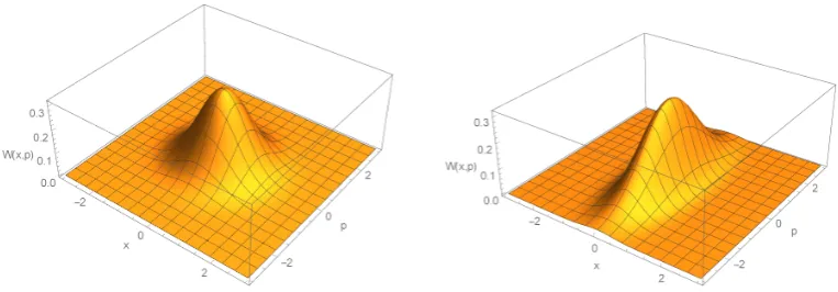
Figure 2.1: Wigner function representations of a vacuum state (left) and squeezed vacuum state in phase-space (right).
state and is defined for [ˆxi,pˆj] =iδi,j as
γlm =
D
ˆ
RlRˆm+ ˆRmRˆl
E
−2hRˆlihRˆmi. (2.52)
One example of a Gaussian Wigner function representation is that of a squeezed state given by the simple equation
W(x, p) = 1
πexp[−x
2e2r−p2e−2r], (2.53)
noting that in the case of a vacuum state the squeezing parameterrwill be zero, both state representations are illustrated in Fig.’s 2.1.
This gives an indication of the simplicity of the Gaussian formalism since states can be fully characterised by their first and second moments. Remarkably, an implication of the Marcinkiewicz Theorem [31–33] is that to fully describe a continuous variable state, one must either only consider the first two moments (as in the case for Gaussian states) or one must consider all of them.
2.3.1
Gaussian Maps
A quantum channel is defined as a quantum operation which is trace preserving [34]. In the most simple instance these operations are reversible and are described by unitary trans-formations U such that U†U = 1l. A Gaussian unitary channel will thus transform one
Gaussian state to another, i.e., it is a Gaussian map.
In the context of phase-space, all Gaussian maps can be represented by a symplectic operation as opposed to a unitary operation in terms of a Hamiltonian. Fig. 2.2 illustrates three transformations of Gaussian states as contours in phase-space, namely a displace-ment, squeezing and a rotation. In order for a symplectic operation to represent a physical operation it must satisfy the condition
SΩS>= Ω ⇒ detS= 1, (2.54)
Figure 2.2: Contours of Gaussian state in phase-space following a Gaussian transformation: (a) displacement of vacuum state gives a coherent state, (b) squeezed vacuum state, (c) rotation of squeezed vacuum state. Dotted circle/ellipse indicates original state and solid shape the post-transformation state.
and Ω is the symplectic matrix given by
Ω = N
M
j=1
ω, ω= 0 1
−1 0
!
. (2.55)
As mentioned previously, some of the most fundamental transformations are Gaussian maps and thus can be represented by a symplectic operation. A rotation in phase-space can be written as
Sr(θ) =
cosθ sinθ
−sinθ cosθ
!
, (2.56)
for some phase shift angleθ. The symplectic squeezing operation can be written as
Ssq(r) =
er 0
0 e−r
!
. (2.57)
wherer is the squeezing parameter equivalent to that defined in Eq.’s (2.35).
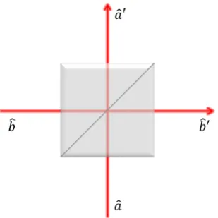
A slightly more sophisticated operation, which will be utilised throughout this Thesis, is a beamsplitter transformation. This will involve a symplectic transformation on two Gaussian modes. A beamsplitter is an optical device allowing the interaction of two input modes, resulting in two output modes consisting of a combination of the input modes (Fig. 2.3). In general, the beamsplitter can have a variable transmittivity to reflectivity ratio, allowing control of the output modes. However a balanced ratio is generally considered as the most common case. In the Heisenberg picture the beamsplitter will transform the annihilation operators, ˆa,ˆb, via a linear non-unitary Bogoliubov transformation as
ˆ
a0
ˆ
b0
!
= T R
R −T
!
ˆ
a
ˆb
!
Figure 2.3: Schematic diagram of a beamsplitter with input modes ˆa, ˆband output modes ˆa0,ˆb0. Physically is a cube made from two triangular glass prisms glued together at their base. The thickness of the resin layer is adjusted such that half of the light incident through one port is reflected and the other half is transmitted due to frustrated total internal reflection.
whereT andRare the transmittivity and reflectivity of the beamsplitter respectively. The symplectic form of the beamsplitter interacting a two-mode system is written in the most general form as
SBS(T, R) =
T 0 R 0
0 T 0 R
R 0 −T 0
0 R 0 −T
, (2.59)
where for the most common case of a balanced beamsplitter T =R= √1
2. A fundamental state which will be discussed is the two mode squeezed vacuum (TMSV) state constructed by the combination, via a balanced beamsplitter interaction, of two orthogonally squeezed vacuum modes, i.e.,
γT M SV =SBS
1/√2,1/√2 Ssq(r)γvacSsq>(r)⊕Ssq(−r)γvacSsq>(−r)
SBS> 1/√2,1/√2.
(2.60) Interestingly, from the aforementioned transformations it is possible to simulate the Einstein-Podolsky-Rosen state as a TMSV in which the positions and momenta of the two modes are maximally entangled3 in the limit of infinite squeezing,r→ ∞.
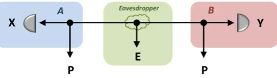
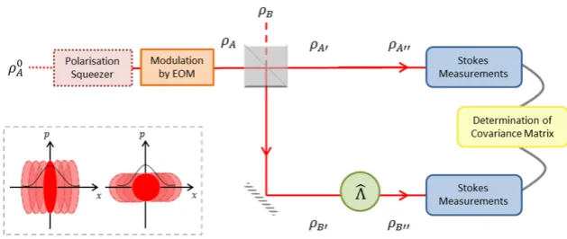
Homodyne and Heterodyne Detection Homodyne and heterodyne are detection pro-cesses for arbitrary squeezed light not restricted to the Gaussian scenario. The concept is to mix the signal field, containing the squeezing, with a strong coherent field known as the local oscillator. Fig. 2.4 illustrates a schematic ofbalanced homodyne detection. As standard with a balanced beamsplitter, the input states (ˆa, ˆb) and output states (ˆc, dˆ) following a
Figure 2.4: Schematic of a balanced homodyne detection with signal ˆaand local oscillator ˆb. Photo-detectors will measure the photo-currents of the output modes and their difference is measured by the photo-current combiner.
beamsplitter interaction are related as
ˆ
a=√1
2(ˆc−i ˆ
d),
ˆb=√1
2( ˆd−iˆc).
(2.61)
Photo-detectors are placed in the output modes and the difference in their intensities is measured, or more specifically, the expectation values of photon operators are compared, i.e.,
hˆncdi=hˆc†cˆ−dˆ†dˆi=ihaˆ†ˆa−ˆb†ˆbi, (2.62) by use of Eq.’s (2.61). Now, since modeb is in a coherent state of the form|βe−iωti, with
β =|β|e−iψ and ψ=θ−π/2, the differences in intensities can be written of the form,
hnˆcdi= 2|β|
1 2
n
ˆ
a0e−iθ+ ˆa†0e iθo
, (2.63)
where ˆa= ˆa0e−iωt. From this, by changing the phase ψof the local oscillator ˆb and hence the angle θ, it is possible to measure a chosen quadrature of the signal field. This angle is generally chosen to yield the maximum level of quadrature squeezing. Heterodyne detection is a similar method of detecting radiation by non-linear mixing with the fundamental differ-ence that the local oscillator will be shifted in frequency, whereas in homodyne detection, the signal field and local oscillator have identical frequencies.
2.3.2
Symplectic Analysis of Gaussian States
γν=SγS>=
j=1 0 νj
, (2.65)
whereνjare the symplectic eigenvaluesdefined as the eigenvalues of|iΩγ|. Due to this, the determinant ofγ is clearly given byQ
jν 2
j. The density matrix representation of a state is connected to symplectic eigenvalues, and by association to the covariance matrix as
ρνj =
N
O
j=1 2
νj+ 1
∞
X
n=0
νj−1
νj+ 1
n
|nij jhn|. (2.66)
Heisenberg’s uncertainty principle can be recast according the symplectic eigenvalues implying that for a physical state, νj ≥ 1 for all j. A particularly important symplectic invariant is the seralian[36], defined in terms of the symplectic eigenvalues,
∆(γ) = N
X
j=1
νj2. (2.67)
An even more simplistic definition for the symplectic eigenvalues and seralian is available when considering bipartite Gaussian states. But first, later in this Thesis the method of purification of a system will become imperative. Holevo and Werner in [37] outlined a procedure for this based on the fact that thermal states are purified by EPR states and derived that for a N-mode Gaussian state ρA, there exist a purifying reference system R such thatρAR is a pure Gaussian state. The covariance matrix of this pure system is given by some symplectic transformationS such that
γAR=
γA SC
S>C> γν
!
where C:= N
M
j=1
p
νj−1σz (2.68)
whereσz is the third Pauli matrix andρA= TrR[ρAR].
Bipartite Gaussian States
Consider a group of systems split across two locations A and B, having N modes andM
modes respectively. The covariance matrix of the entire system can be put into the general form
γ= γA γC
γC> γB
!
where γA is a 2N ×2N matrix, γB a 2M ×2M matrix and γC contains the correlations between modes at locationsAandB.
Throughout the course of this Thesis a focus will be put on the instance where only a single mode will be present at location A and B. In this simple case there exists a local symplectic transformation that will transform any covariance matrix into standard form defined as
γsf =
a 0 c+ 0
0 a 0 c−
c+ 0 b 0
0 c− 0 b
. (2.70)
with the correlation elements satisfyingc+=−c−:=c≥0.
The local invariants of the standard form matrix can be expressed in terms of these matrix elements as
det(γsf) = (ab−c2+)(ab−c2−), ∆(γsf) =a2+b2+ 2c+c−, (2.71)
and the symplectic eigenvalues are given by
ν±=
s
∆±p
∆2−4 det(γ sf)
2 (2.72)
The particular significance of these invariants in relation to quantum correlations will become apparent in Chapter 3. Furthermore, purity — or rather the degree of mixedness of the state — can be tested for bipartite systems from its covariance matrix such that if
µ= p 1
det(γ)= 1, (2.73)
the state is pure and for 0 ≤ µ < 1 the state is mixed. For systems containing three subsystems the purification of the system is valid if,
∆ij = detij+ 1, (2.74)
or using entropies
S(ρij) =S(ρk), (2.75) hold for all permutations of the subsystems.
It is now necessary to link this quantum mechanical representation of physical states to a fundamental concept and tool within quantum information processing, that of entropy.
2.4
Entropy and Quantum Information
as
Iq(ρAB) =S(ρA) +S(ρB)− S(ρAB), (2.76) whereS(ρA) denotes the marginal entropy of subsystemAandS(ρAB), the joint entropy of states. Specific measures of entropy, both classical and quantum, will be defined in Section 2.4.1. The quantum mutual information thus captures all of the information of states ρA andρB composing the larger composite stateρAB.
The classical correlation in a quantum system is defined as the difference in marginal entropy of one subsystem after a measurement is performed on the remainder of the system, and is operationally related to the amount of perfect classical correlations which can be extracted from the system [39], i.e.,
J(ρAB) =S(ρA)− inf
{Πˆj}H{Πˆj}(ρA|ρB), (2.77)
where inf{Πˆ
j}H{Πˆj}(α|β) corresponds to the quantum conditional entropy, the entropy of
the first subsystem subject to a measurement on the second, optimised over all possible measurements. The specific set of measurements that will be considered in the Thesis will be discussed later in Section 4.1.1. A direct result of this is that, in a purely classical system,
I(ρAB) =J(ρAB)
⇒ S(ρAB) = inf
{Πˆj}H{Πˆj}(ρA|ρB) +S(ρB),
(2.78)
thus the joint entropy of the system is the sum of the conditional entropy of subsystemA
and the marginal entropy of subsystemB, such that ifAis undisturbed by a measurement onB then the joint entropyS(ρAB) will be zero.
2.4.1
Entropic Measures
So far entropy has been referred to as a general concept and quantity. This Section aims to provide an outline of two significant entropic measures namely the famous von Neumann entropy [40, 41] and the lesser known R´enyi-2 entropy, both introduced as special cases of the R´enyi-αentropy.
R´enyi-αentropies were first introduced by Alfr´ed R´enyi as a generalisation of the usual concept of entropy [42]. These entropies not only encompass the Hartley (or max) entropy, min-entropy and collision entropy, but also the Shannon entropy [43] and consequently, the von Neumann entropy. More recently preliminary work has been done to link the R´enyi-α
defined as
Hα(P) = 1 1−αlog2
N
X
k=1
pαk
!
, α >0 and α6= 1, (2.79)
where P is a distribution P = (p1, p2, . . . , pN). By implementation of L’Hˆopital’s Rule4 in the limit of α→1, Eq. (2.79) reduces to the Shannon entropy as
H1(P) = lim
α→1Hα(P) = N
X
k=1
pklog2 1
pk
. (2.80)
The quantum analogue to the R´enyi-αentropy is given by
Sα(ρ) = 1
1−αln Tr(ρ
α) (2.81)
whereρis the density matrix describing a quantum state. Considering again the case when
α→1, Eq. (2.81) will reduce to the von Neumann entropy introduced as quantifying the departure of the system from a pure state and defined as
S1(ρ) =−Tr[ρlnρ]. (2.82)
Consequently, for anN-mode Gaussian state the von Neumann entropy is calculated as
S(ρ) = N
X
j=1
f(νj), (2.83)
whereνj are the symplectic eigenvalues and
f(x) =
x+ 1
2
ln
x+ 1
2
−
x−1
2
ln
x−1
2
. (2.84)
is a monotonically increasing function of x. The von Neumann entropy has the properties of both subadditivity, given by
|S(ρA)− S(ρB)|≤ S(ρAB)≤ S(ρA) +S(ρB), (2.85)
and strong subadditivity, given by
S(ρABC) +S(ρB)≤ S(ρAB) +S(ρBC) ⇔ S(ρA) +S(ρC)≤ S(ρAB) +S(ρBC). (2.86)
In recent publications, focus has increasingly been placed on the significance of the case when α = 2. It is suggested that this so-called R´enyi-2 entropy is a much more natural entropic measure of a quantum state, particularly within the Gaussian setting. Considering the instance whenα= 2, the entropy is of the formS2(ρ) =−ln Tr[ρ2]. At first glance it is
4L’Hˆopital’s rule states that for two differentiable functionsfandgon an open intervalI: lim
x→∞fg((xx)) = limx→∞f
The question of whether the von Neumann entropy is the most natural of entropies arises from the fundamental conjecture that the minimum output entropy conjecture for bosonic channels, proven for all R´enyi-α entropies for α≥ 2 [29, 45–47]. Most recently it has also been proven for the case ofα→1 i.e., the von Neumann entropy, by Giovannettiet al.[48]. It has been shown in [49] that the R´enyi-2 entropy arises naturally from phase-space sampling for Gaussian states as
H(Wρ) =−
Z
R2N
Wρ(ζ) ln [Wρ(ζ)]d2Nζ
=
Z
R2N 1
πN√detγexp −ζ
>γ−1ζ
ζ>γ−1ζ+Nlnπ+1
2ln(detγ)
d2Nζ
= 2N
X
j=1
νj 2νj
+Nlnπ+S2(ρ)
=N(1 + lnπ) +S2(ρ)
(2.88)
where an integration has been performed in phase-space coordinatesζsuch thatγis diago-nalised,νj are the eigenvalues of the matrix andN =nA+nB is the total number of modes of the composite system. This can be extended to represent Shannon relative entropy as
H(Wρ1k Wρ2) =
Z
R2N
Wρ1(ζ) ln
Wρ1(ζ)
Wρ2(ζ)
d2Nζ
=−H(Wρ1) +
Z
R2N 1
πN√detγ
1
exp −ζ>γ1−1ζ
ζ>γ2−1ζ+Nlnπ+1
2ln(detγ2)
d2Nζ
=1 2ln
detγ
2 detγ1
−N+ 2N
X
j=1
γ1,jj 2γ2,j
=1 2 ln detγ 2 detγ1
+ Tr γ1γ2−1
−N
(2.89)
where γn,j denote the eigenvalues of γ, and γn,ij are its individual matrix elements. The validity of the final step is due to the invariance of the quantity Tr
γ1γ2−1
under a change of basis.
andρB. The quantum mutual information between these two subsystems can be written as
H(WρAB k WρA⊗ρB) =H(WρA) +H(WρB)− H(WρAB)
= 1 2ln
detγ
AdetγB detγAB
=S2(ρA) +S2(ρB)− S2(ρAB) =I2(ρA:B),
(2.90)
since Tr
γ1γ2−1
= 2N. It is clear that this is analogous to the von Neumann definition of mutual information Eq. (2.76). This Gaussian R´enyi-2 mutual information is positive semi-definite as it coincides with the Shannon mutual information of the Wigner function ofρAB and has the operational interpretation of the total quadrature correlations of the composite state ρAB since Eq. (2.90) describes the required extra amount of discrete information to be transmitted over a continuous variable channel which will allow the construction of the complete joint Wigner function ofρAB as opposed to the two marginal Wigner functions.
In Ref. [50] the development of the Gaussian R´enyi-2 formalism was extended further to include a quantum conditional entropy optimised over all single mode Gaussian mea-surements. Any measurement considered is described by positive operator valued measure (POVM)5 of the general form onn
B modes
ΠB(η) =π−nB
nB Y j=1 ˆ
WBj(ηj)
ρ Π B nB Y j=1 ˆ
WB† j(ηj)
(2.91)
where ˆW is the Weyl displacement operator
ˆ
WB(ηj) = exp
ηjˆb†j−η ∗ jˆbj
, ˆb j = 1 √
2 qˆBj +ipˆBj
,
π−nB
Z Y
B
(η)d2nBη= 1l
(2.92)
and ρΠ
B is the density matrix of a nB-mode mixed Gaussian state with covariance matrix ΓΠB. The covariance matrix of the conditional state ofAwhen a measurement is performed on subsystemB is given by the Schur complement
˜
γAΠ=γA−γC(γB+ΓΠB)− 1γ>
C. (2.93)
5A positive operator valued measure (POVM) is a measure with elements which are non-negative
such as the quantum mutual information, in Eq. (2.90), can become negative, and so is then a meaningless correlation measure. However, R´enyi-2 entropy satisfies a strong subadditivity inequality for all Gaussian statesρABC,
S2(ρAB) +S2(ρBC)≤ S2(ρABC) +S2(ρB),
⇒1
2ln
detγ
ABdetγBC detγABCdetγB
≥0. (2.95)
The consequence of this is that the core of quantum information theory can be consistently recast within the Gaussian scenario, using the simpler and physically natural R´enyi-2 entropy as opposed the von Neumann entropy.
Quantum Entanglement
The birth of quantum entanglement is considered to have taken place in 1935 when Ein-stein, Podolsky and Rosen published a paper entitled “Can quantum-mechanical description of physical reality be considered complete?”, of which the answer was no [4]. It was consid-ered that if in the case of two physical quantities described by non-commuting operators (position and momentum), the knowledge of one precludes the knowledge of the other, then the quantum mechanical theory of physical reality must be incomplete. At the time of the EPR paper, the quantum mechanical interpretation of physical reality was challenged by local realism. “Realism” implies the existence of a probability distribution dependent on how the global state is generated and thus that there must be a pre-existing outcome for any pos-sible measurement before the measurement is made. “Locality” implies that a measurement choice and outcome of one subsystem should not impact the result of a measurement on the remaining subsystem. This interpretation was proved to be contradicted by the EPR para-dox. The concept explored in this thought experiment is: given two quantum systems, if the information contained in the entire system cannot simply be described by each subsystem individually, then the additional information contained therein defines quantum entangle-ment. By this, it can be stated that one subsystem cannot be fully understood without considering its counterpart. Einstein found the apparent “spooky action at a distance” (or “spukhafte Fernwirkung”) [51] to be contradictory to reality and was fundamentally uncom-fortable with the concept of its validity. The same year, in the journal Naturwissenschaften, Schr¨odinger coined the term “Verschr¨ankung”, meaning “entanglement”. Schr¨odinger de-veloped his famous thought experiment of a cat, which exists simultaneously in a state of being alive and dead, to help illustrate the difference in classical and quantum mechanics, and in turn the concept of quantum superposition exhibited by an entangled state [5].
In 1952, building on earlier work by de Broglie [52], Bohm suggested a deterministic interpretation of quantum theory that incorporates “hidden variables” [53], the values of which effectively determine, from the moment of separation, the outcomes of the measure-ment. Implying that each particle carries all the necessary information and no information is required to be transmitted from one system to the other at the time of measurement.
It was then in 1964 that Bell proposes his famous theorem allowing researchers to later experimentally, and definitively, rule out any hidden variables operating locally to justify
effects do exist [59–61].
Fundamental applications of quantum entanglement were then introduced from 1984 in the form of quantum cryptography, which would use photons from an entangled system to create a secure key [62]. It was also found in 1993 that entanglement can be used to teleport a particle’s quantum information from one place to another [63], first experimentally verified separately by Zeilinger and De Martini groups (1997–1998) [64, 65]. The distance record of sending entangled photons across 144 kilometers, between two of the Canary Islands, was set in 2007 by Zeilinger’s group [66].
The improved comprehension of quantum entanglement has been remarkable in the past two decades. The phenomenon is no longer one which exists between photons or electrons, the effects of quantum entanglement have been witnessed between vibrational states of two spatially separated, millimetre-sized diamonds at room temperature [67]. The dimensional limit to which entanglement can persist appears to be expanding with quantum proper-ties such as wave-particle duality been found in molecules the size of Buckminsterfullerenes (or Bucky-balls)1 [68]. Research involving practical purposes of quantum entanglement are becoming ever more popular as the world edges closer to the inevitable development of physical quantum technologies, including quantum computers [69] and quantum cryptogra-phy [70, 71].
3.1
Characterising Bipartite Entanglement
3.1.1
Bell’s Inequality and Local Realism
Let us consider a hypothetical world in which local realism is the valid interpretation of the physical world and focus on a bipartite system within this world. Each systemSAand
SB will have two parameters assuming the values s(n,1) and s(n,2) respectively, which are independent of observation, wheren corresponds to an individual system. In this instance Bell’s CHSH inequality [55] will read as
|hs(A,1)s(B,1)i+hs(A,1)s(B,2)i+hs(A,2)s(B,1)i − hs(A,2)s(B,2)i|≤2 (3.1)
wherehs(A,j)s(B,k)iis the average over the case wheres(A,j)is measured, and simultaneously,
s(B,k)is also measured. This inequality is born from the probability distribution dependent on how the global state is generated. However in quantum mechanics, in the majority of cases if the system possesses entanglement, Bell’s inequality will be violated yielding a value
1Bucky-balls are spherical fullerene molecules with a cage-like structure made of twenty hexagons and
of 2√2>2, although there exist so-called Werner state for which this is not the case. The set of states which provide a saturation of this inequality, appropriately known asBell states. These represent maximally entangled bipartite states, defined as,
|Φ±i=√1
2(|s(A,1)s(B,1)i ± |s(A,2)s(B,2)i), (3.2a)
|Ψ±i= √1
2(|s(A,1)s(B,2)i ± |s(A,2)s(B,1)i). (3.2b)
3.1.2
Definition of an Entangled State
The definition of quantum entanglement was put forward as a contradiction. That is, an entangled state is one which cannot be considered as separable and thus written as a tensor product of the density matrices of its subsystems [72, 73]2,
ρAB =
X
j
pjρA,j⊗ρB,j, (3.3)
where ρn,j is the density matrix of subsystemnandpj is its associated probability. Hence it appears that entanglement is equivalent to non-separability.
Within the covariance matrix formalism for Gaussian states, it was shown by Werner and Wolf [74] that a bipartite state is considered separable if it can be expressed as a direct sum of the covariance matrices of the subsystems, i.e. a product state
γAB≥
γA 0
0 γB
!
. (3.4)
In the case of the inequality being saturated, the covariance matrix will correspond to a state which solely possesses classical correlations and thus exhibits no quantum entanglement. This qualitative definition holds only with respect to pure states, however the more complex case of mixed sates is discussed in Chapter 4.
Local Operations and Classical Communication (LOCC)
One of the most important properties of quantum entanglement is its Local Operations and Classical Communication (LOCC) constraint. Considering two states which are per-fectly entangled, the presence of entanglement would be synonymous to a perfect quantum communication channel. In actuality however, noise will inevitably play a detrimental role to this communication channel. One option to counteract these noisy channels is to use LOCC, which can be used to form classical correlations. If a bipartite quantum state is then used to successfully perform a particular task which cannot be explained by classical correlations alone, the solution must be that the ability to perform the task must be due
2In Ref. [72] Werner used the words “classically correlated”, but the term “separable” was chosen by
are said to be maximally entangled. These states by definition yield a maximally mixed state when one subsystem is traced out. However in an infinite-dimensional Hilbert space, a maximally entangled state could only be achieved by taking, for example, a two-mode squeezed vacuum state in the limit of infinite squeezing, r→ ∞. For any entangled state, the constraint on entanglement is that it cannot emerge nor increase under LOCC operations, although a local unitary operation may have the effect of decreasing entanglement.
3.2
Separability Criteria
As discussed, the definition of an entangled state, and hence entanglement, is based on the concept that if a state cannot be classified as separable, it is entangled. Arising from this are a number of separability criteria which serve as a verification of the presence or absence of entanglement. It is important to note that the resolution power of different separability criteria can vary, leading to an objective definition of the ‘border’ between separable and entangled states, such that separable according to one criteria can appear non-separable according to another.
Before introducing the main separability criterion used within this Thesis, it is necessary to present the notion of a positive but not completely positive map. A positive map, as the name suggests, will act in such a way as to transform a positive matrix3 i.e. the density matrix, to another positive matrix. The positivity of the resulting state determines its validity as a quantum state. In addition, a map Z is positive if it preserves the property of being Hermitian. Considering a bipartite system with density matrix ρAB, using Choi’s theorem [75], a mapZ is defined as positive if,
(1l⊗Z)ρAB = (1l⊗Z)
X
j
pjρA,j⊗ρB,j
=
X
j
pjρA,j ⊗ZρB,j. (3.5)
If the resulting density matrix is positive, the map is known ascompletely positive. However, to utilise this theorem for the purposes of identifying entanglement, those maps which are positive but not completely positive are of interest. A quantum state is then considered to be separable if and only if
(1l⊗Z)ρAB≥0, (3.6)
for positive but not completely positive maps.
3.2.1
Peres-Horodecki Criterion (PPT)
One of the most recognised separability criteria for bipartite and multipartite quantum systems is the Peres-Horodecki criterion [76, 77]. Popularly known as the PPT criterion due to its use of a positive partial transpose4, this criterion is based on a positive but not completely positive map. It was demonstrated in [77] that the PPT criterion is necessary and sufficient for quantum statesρAB defined in the Hilbert space HAB =HA⊗ HB as in Eq. (3.3) for dimensionsdA= 2 or 3 anddB= 2 where the PPT of one subsystem, sayρA, simply defined by the density matrix
ρ>A
AB =
X
j
pjρ>A,j⊗ρB,j, (3.7)
corresponds to a valid density matrix, with the superscript >n indicating with respect to which subsystem the transpose is being performed. It was also shown that the Peres-Horodecki criterion is sufficient for separability whendA·dB ≤6.
The Peres-Horodecki criterion has been extended to continuous variable systems by Si-mon [78], where it is interpreted as the time reversal of one subsystem. Consider a bipartite state with a covariance matrix basis (xA, pA, xB, pB), PPT on subsystemB will result in a change of basis as (xA, pA, xB, −pB). Note that although performing a time reversal on an individual quantum system will lead to a valid density matrix, this is not guaranteed when performing time reversal on a subsystem of a larger global system.
In respect to the symplectic formalism for Gaussian states, PPT can be represented by a symplectic Gaussian map as
λA|B =
N
M
j=1 1lj
⊕
M
M
k=1
σz,k
!
(3.8)
where N and M denote Hilbert dimensions of subsystems A and B respectively and σz is the third Pauli spin matrix. From Ref. [78] the separability criterion for a bipartite Gaussian state is fully characterised by the lower symplectic eigenvalue of the partially transposed system, ˜ν−. The stateρAB is considered separable if and only if ˜ν−≥1, thus ˜ν−
fully characterises the entanglement, a fact which is considered in a later following Section introducing a range of basic entanglement measures.
3.2.2
Other Separability Criteria
This Section will serve as a brief introduction to other popular existing separability criteria, chosen due to their simplicity as well as their frequent use in literature [79].
4The partial transpose simply refers to the transpose of one subsystem whilst the remaining subsystems
m m
for∀m >0 andm∈R, the variance of these operators is then given by
h(∆ˆu)2iρ+h(∆ˆv)2iρ≥m2+ 1
m2. (3.10)
The Gaussian counterpart relies on the state being expressed in a standard form covariance matrix similar to Eq. (2.70) but with a1 6= a2 and b1 6=b2. The operators then become [81, 82]
ˆ
u=|m0|xˆ1−
c+
|c+| 1
m0
ˆ
x2, and vˆ=|m0|pˆ1−
c− |c−|
1
m0
ˆ
p2, (3.11)
wherem0= 4
r
b1−1
a1−1
= 4
r
b2−1
a2−1
and so the inseparability criterion becomes,
m20a1+a2
2 +
b1+b2 2m2
0
− |c+|−|c−|≥m20+ 1
m2
0
. (3.12)
for bipartite Gaussian states.
Range Criterion
Consider a state ρAB where the dimensions of the two subsystem yielddA·dB >6. In this case there exists states that are entangled but separable according to PPT, therefore another, separability criterion is required to detect the entanglement of these states independent of the PPT criterion. One such criterion based on positive but not completely positive maps where the chosen map is not decomposable is the range criterion [83].
The range criterion states that if the stateρAB is separable, then by definition, there exists a set of product vectors {ψi
A⊗φiB} that span the range ofρAB, while{ψAi ⊗(φiB)∗} spans the range of the partial transpose ρ>B
AB, where the complex conjugate is taken in the same basis as the partial transposition on ρAB.
Reduction Criterion
A reduction map is defined as a linear map Λr :SdA×dB → SdA×dB such that Λr[ρAB] =
1l(Tr[ρAB])−ρAB, withρAB∈ SdA×dB and 1l the identity operator. The reduction criterion
[84, 85] then states that if a state ρAB ∈ SdA×dB is separable, then (1l⊗Λr)[ρAB]≥0, i.e.,
the following two conditions hold