Genetic algorithm for biobjective urban transit routing problem

(1)

Volume 2013, Article ID 698645,15pages http://dx.doi.org/10.1155/2013/698645

Research Article

Genetic Algorithm for Biobjective Urban Transit

Routing Problem

J. S. C. Chew,

1

L. S. Lee,

1,2

and H. V. Seow

3

1_{Department of Mathematics, Faculty of Science, Universiti Putra Malaysia, (UPM), 43400 Serdang, Selangor, Malaysia} 2_{Institute for Mathematical Research, Universiti Putra Malaysia, (UPM), 43400 Serdang, Selangor, Malaysia}

3_{Nottingham University Business School, University of Nottingham Malaysia Campus, Jalan Broga,} 43500 Semenyih, Selangor, Malaysia

Correspondence should be addressed to L. S. Lee; [email protected]

Received 14 June 2013; Revised 21 October 2013; Accepted 21 October 2013

Academic Editor: Julián López-Gómez

Copyright © 2013 J. S. C. Chew et al. This is an open access article distributed under the Creative Commons Attribution License, which permits unrestricted use, distribution, and reproduction in any medium, provided the original work is properly cited.

This paper considers solving a biobjective urban transit routing problem with a genetic algorithm approach. The objectives are to minimize the passengers’ and operators’ costs where the quality of the route sets is evaluated by a set of parameters. The proposed algorithm employs an adding-node procedure which helps in converting an infeasible solution to a feasible solution. A simple yet effective route crossover operator is proposed by utilizing a set of feasibility criteria to reduce the possibility of producing an infeasible network. The computational results from Mandl’s benchmark problems are compared with other published results in the literature and the computational experiments show that the proposed algorithm performs better than the previous best published results in most cases.

1. Introduction

The urban transit network design problem (UTNDP) is concerned with searching for a set of routes and schedules according to the predefined stations and passengers’ demand in each station for an urban public transport system. The UTNDP is a complex NP-hard problem where a lot of criteria need to be met in order to maximize the passengers’ satisfaction and at the same time minimize the cost of the service provider [1].

Chakroborty and Dwivedi [2] divided the UTNDP into two major components, namely, the urban transit routing problem (UTRP) and the urban transit scheduling problem (UTSP). In general, the UTRP involves searching for an efficient transit route (e.g., bus routes) on existing road networks and nodes, with predefined pick-up/drop-of points (e.g., bus stops), following certain constraints. In a transit network, adjacent nodes are linked by an arc or edge, and a route will consist of several nodes connected by edges to form a path. One or more such routes can be combined to form a route set, and when all the routes in a route set are superimposed, this will form a route network. After an

efficient route network has been found, the UTSP will act to find an efficient schedule for that route set. Due to the complexity of the UTNDP, Chakroborty and Dwivedi [2] stated that solving both the transit routing and scheduling concurrently is not felt to be possible. Therefore, the UTRP and UTSP are usually implemented sequentially with the UTRP coming before the UTSP. More recently, Fan et al. [3] stated in their work that the UTRP is a highly complex multiconstrained problem where the evaluation route sets can be very time-consuming and challenging as well. Many potential solutions were rejected due to infeasibility.

(2)

there is no single solution that best represents both parties. In this case, the optimal solution is called a Pareto optimal solution where there exists no other feasible solution which would decrease some objectives (in a minimization problem) without causing a simultaneous increase in at least one other objective [4].

We address the biobjective UTRP using a genetic algo-rithm (GA) approach. In the proposed algoalgo-rithm, the initial population is being initialized with the help of Floyd’s algorithm [5]. Every individual must go through four feasible criteria in order to ensure the feasibility of each individual. For the genetic operators, route crossover and identical-point mutation are proposed. The biobjective UTRP is solved sequentially by switching the objective function after the first objective has converged. Each of the contributions will be explained later in the paper.

In the following section, the literature review of the UTRP is given, followed bySection 3where we explain the objective functions and constraints. Our proposed GA will be discussed in Section 4. The computational results and discussions will be presented inSection 5. Finally, the paper ends with a conclusion inSection 6.

2. Literature Review

There are many approaches for solving the UTRP. It would not be possible to cover the literature involved for the scope of this paper. Thus, this section will focus mainly on the use of the evolutionary algorithms, particularly GA for multiobjective UTRP.

Pattnaik et al. [6] solved the multiobjective problem by minimizing both passengers’ and operators’ costs using a GA. They designed the algorithm by involving route configuration and also associated frequencies to achieve the desired objec-tives. The proposed algorithm is implemented in two phases. First, a set of candidate routes that are going to compete to be the optimum solution is generated by a candidate route set generation algorithm (CRGA). Then, the optimum solution is selected through the GA. In the second phase, the route evaluation module is used to evaluate the objective function value. Two models based on the GA were developed: the fixed string length coded model and the variable string length coded model. They applied the algorithm to a transportation network in part of the Madras Metropolitan City, South India, with 25 nodes and 39 links.

In 2001, Chien et al. [7] presented two methods, a GA and an exhaustive search algorithm, to optimize the biob-jective UTRP and its operating headway while considering intersection delays and realistic street patterns. The aim of Bielli et al. [8] is to improve the old performance of a bus system network by trying to reduce the average travel time of the passengers and the management costs through the reduction of the number of vehicles employed in the network. In the first step, they implement a simple GA. A classic assignment algorithm is used to evaluate the fitness function. The assignment phase is when the improvement of the results occurs and where a neural network approach will be used to compare the results. Finally, the cumulative GA adopted from Xiong and Schneider [9] is performed.

Later in 2002, Bielli et al. [10] solved the biobjective problem that involved satisfying both the demand of the passengers and the offer of the transport by using GA. Their goal was to design a bus route network associated with frequencies. The proposed algorithm is then applied to a small city located in the middle-north of Italy. In the same year, Fusco et al. [11] minimized the overall system costs of the UTNDP. They attempted to design a transit network that consists of a set of routes and the associated frequencies. The designer’s own knowledge was also adopted into the algorithm. The proposed GA combines the transit network design methods developed by Baaj and Mahmassani [12] and Pattnaik et al. [6].

Tom and Mohan [13] searched for a set of routes and the associated frequencies with an objective to minimize the operating cost and the passenger total travel time. In the paper, they separated the model into two distinct phases. Candidate route generation algorithm is used to generate a large set of candidate routes in phase one. Phase two involved a GA to select the solution route set. The proposed GA is then validated on a network which is part of the Chennai Metropolitan City, South India, with 75 nodes and 125 links.

Ngamchai and Lovell [14] have designed seven different genetic operators for their GA. The objective of the paper was to demonstrate the efficiency of the problem-specific genetic operators in optimizing the UTRP which include passengers’ cost and operators’ cost incorporating frequen-cies settings for each route. The proposed model consists of three major components:(1)route generation algorithm to construct a feasible initial population,(2)route evaluation algorithm where the overall cost is calculated, and (3) route improvement algorithm where modification is applied to the current route set by using the seven genetic operators with the hope to discover a better route set. The network configuration from Pattnaik et al. [6] is used to measure the performance of this proposed model.

Fan et al. [3] initialize their route set by first constructing a random route. Then, they chose to start the first node of the subsequent routes from the set of nodes present in the previously constructed routes. For the next node, the procedure will favor nodes that have not appear in the route set. This procedure is to minimize the probability of getting an infeasible route set. However, if a route set is not feasible, the make-small-change procedure is utilized repeatedly until a feasible route set is found. They presented the simple multiobjective optimization algorithm to solve the multiobjective UTRP. The scheme is based on the SEAMO algorithm proposed by Valenzuela [15] and Mumford [16], but without the crossover operator.

(3)

Most recently, Mumford [18] has presented some new sophisticated problem-specific heuristics and genetic oper-ators for the UTRP in a multiobjective evolutionary frame-work. The approach balances passenger and operator costs. Computational results on Mandl’s benchmark have outper-formed the previous best published results by Fan et al. [3] for the passenger costs and equaled the lower bound for operator costs.

3. The Urban Transit Routing Problem

The UTRP involves determining a set of efficient transit routes that meet the requirements of both passengers and the operator. For simplicity purposes, in this paper, only symmetrical transit networks are considered, in which the travel time, distance, and demand between two nodes are the same regardless of the travel direction. The basic problem representation given by Fan et al. [3] is as follows.

The transit network is represented by an undirected graph

𝐺(𝑉, 𝐸)where the nodes𝑉 = {𝑥₁, . . . , 𝑥_𝑛}represent access

points (e.g., bus stops) and the edges 𝐸 = {𝑒₁, . . . , 𝑒_𝑚} represent direct transport links between two access points. A route can then be represented by a path in the transit network,

𝑟_𝑎= (𝑥_𝑖₁, . . . , 𝑥_𝑖_𝑞) , where𝑖_𝑘∈ {1, . . . , 𝑛} , (1)

and a solution to the UTRP is specified by a route set:

𝑅 = {𝑟_𝑎: 1 ≤ 𝑎 ≤ 𝑁} . (2)

A route network is associated with a route set to be the subgraph of the transit network containing precisely those edges that appear in at least one route of the route set.

The efficiency of public transport from the passengers’ point of view includes a low travel time from the source to the destination and the number of transfers involved being as low as possible or no transfer at all. This is because transfer waiting time will eventually increase the travel time of the passengers. It is a difficult task to optimize the transit network due to the complexity of the transit travel time characteristics which include vehicle travel time, waiting time, transfer time, and transfer penalties. From the operators’ point of view, however, the objective is to minimize the cost in operating the service to make as much profit as possible. It is a challenge in the UTNDP to find an equilibrium between these two conflicting objectives, not forgetting other expectations for an efficient public transport system from other points of view such as the local government and the community. Therefore, the definition for efficiency might be different according to various points of view.

According to Chakroborty and Dwivedi [2], the aim of the UTRP is to serve transit demand efficiently. An efficient route set is one that satisfies the following.

(1) The route set should satisfy all of the transit demand. (2) The route set should satisfy the transit demand of passengers with the percentage of demand satisfied with zero transfer to be as high as possible.

(3) The route set should offer an average travel time per transit to be as low as possible.

From the passengers’ point of view, the objective function is the total travel time made by all the passengers that travel from their source to their respective destination (Fan et al. [3]):

Minimize 𝐶_𝑃=

𝑖=𝑛−1

∑

𝑖=1 𝑗=𝑛

∑

𝑗=𝑖+1

𝑑_𝑖𝑗𝑡_𝑖𝑗, (3)

where𝑑_𝑖𝑗is travel demand between node𝑖and node𝑗and𝑡_𝑖𝑗 is the shortest travel time between node𝑖and node𝑗.

From the operators’ perspective, the running cost in operating the public transport is an important consideration. Operators aim to minimize the cost in operating the service. Operators will try to minimize the route length so as to reduce the fuel costs and also reduce the mileage of the public transport which directly affect the maintenance frequencies of the public transport. Thus, it is clear that the total route length of a public transport system is an important aspect for the operator’s cost. The objective function from the operators’ perspective is proposed by Fan et al. [3]:

Minimize 𝐶_𝑂=

𝑟

∑

𝑙=1

𝐿𝑙, (4)

where𝑟is total number of routes in the route set and𝐿_𝑙 is length of route𝑙.

Both of the objective functions are subject to the following constraints.

(1) The number of nodes in a route must have a minimum number of two nodes and must not exceed the predefined maximum number of nodes set by user in a route.

(2) There must be exactlyxnumber of routes in a route set which is predefined by the user.

(3) Each route in the route set is free from repeated nodes. This is to avoid backtracks and cycles of a route. (4) All nodes must be included in the route set in order

to form a complete route set.

(5) The routes in the route set are connected to each other. (6) The exact same route cannot be repeated in a single

route set.

(7) The demand, travel time, and distance matrices are symmetrical, and we assume that a vehicle will travel back and forth along the same route, reversing its direction each time it reaches a terminal node. (8) The demand level remains the same throughout the

period of study.

(9) The transfer penalty (representing the inconvenience of moving from one vehicle to another) is set at 5 minutes.

(4)

(11) Passenger choice of routes is based on the shortest travel time.

In the literature of the UTRP, the problem has been char-acterized with different optimization criteria and constraints. However, the following parameters have been adopted by many researchers to assess the quality of the route set (Mandl [19], Baaj and Mahmassani [20], Kidwai [21], Chakroborty and Dwivedi [2], and Fan and Mumford [22]):

𝑑₀: percentage of demand satisfied without any transfers,

𝑑₁: percentage of demand satisfied with one transfer,

𝑑2: percentage of demand satisfied with two transfers,

𝑑_𝑢𝑛: percentage of demand unsatisfied (we assume that more than two transfers per journey are unaccept-able),

ATT: average travel time in minutes per transit user incor-porates transfer penalty of 5 minutes per transfer.

These parameters will be used to measure the quality of the final biobjective results produced by the proposed algorithm.

4. Genetic Algorithm

The proposed GA starts with an initial set of solutions called population. Each solution in the population is called an individual which is initialized with the help of Floyd’s algorithm. Every individual will need to go through four feasible criteria for the feasibility purpose. In each generation, individuals will be selected to perform the genetic opera-tions of crossover and mutation. Inspired by Chakroborty and Dwivedi [2] and Ngamchai and Lovell [14], the route crossover and identical-point mutation are introduced. The steady-state replacement strategy is adopted where a new generation is formed by selecting a subset of parents and offspring according to their fitness values and by rejecting others to keep the population size constant. To solve the biobjective UTRP, both of the objectives are implemented sequentially by using the same set of initial population. When all the chromosomes have converged, it indicates that the implementation has reached the stopping criteria. The final solution hopefully represents the optimal solution or a near-optimal solution to the problem. In the remainder of this section, each GA component of the proposed algorithm is explained in detail.

4.1. Initialization. A complete route set consists of more than one route forming from a list of nodes. Thus, to initialize the population, the nodes are listed in the order in which they are visited by using one dimensional integer representation array where each route is separated by a “0”. For example, if the integer representation of a route set is

1 3 4 0 2 6 5 0,

then there are two routes in the route set where the first route will first visit node 1, followed by node 3 then finally node 4 before returning to nodes 3 and 1. This can be interpreted by using the notations 1-3-4 and 2-6-5 for the first and second

routes, respectively. Note that a feasible network is made up by a minimum number of two nodes in a route and a predefined number of maximum nodes in a route by the user. To initialize an individual, firstly, two random nodes will be generated. The first node represents the starting point while the other one represents the destination point of the route. Floyd’s algorithm [5] is embedded to help find the shortest distance between two randomly generated nodes if both of the nodes are not connected to each other. The process is repeated until the predefined number of routes has been reached to form a partial route set. Following this, a complete route set can be found by executing the feasibility check in order to ensure the feasibility of the route set. The proposed GA will initialize a fixed number of population which is, in our case, 200 individuals and the population size (𝑃pop) is kept constant throughout the implementation.

4.2. Feasible Criteria. The feasibility check is important in generating a feasible initial population before proceeding to the genetic operations. There are four criteria that need to be fulfilled by the route set in order to generate a feasible solution.

(I) A Node Can Never Be Repeated Twice in a Route but Can Be Repeated in The Network. As mentioned before, during the chromosome initialization stage, two random numbers are generated; the first number represents the first node of the route and the second number represents the last node of the route. If both nodes are not connected to each other, then Floyd’s algorithm [5] is used to find the shortest distance between the two nodes. The steps are repeated until the required number of routes reached. This way actually enables us to produce a route without a repeated node. Unfortunately, a problem can occasionally arise when the length of the route is longer than the predefined maximum nodes allowed in a route causing the route to be infeasible. Hence, in this situation, another new route will be selected to replace this infeasible route.

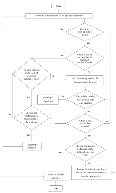
(II) A Complete Network Allows No Missing Node.The missing node refers to the node that cannot be found in the network. This is when the adding-node procedure is introduced. The idea of this procedure is to add the missing node into the network without violating criteria I. As mentioned, Floyd’s algorithm is used to construct a partial network. For example, if node𝑥 is missing from the partial network of

1 2 3 5 0 5 6 0 with the maximum number of 4

(5)

[image:5.600.51.290.82.148.2]

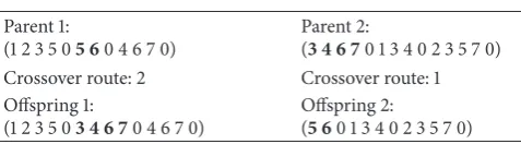
Table 1: Route crossover.

Parent 1:

(1 2 3 5 05 6 0 4 6 7 0)

Parent 2:

(3 4 6 7 0 1 3 4 0 2 3 5 7 0)

Crossover route: 2 Crossover route: 1

Offspring 1:

(1 2 3 5 03 4 6 7 0 4 6 7 0)

Offspring 2:

(5 6 0 1 3 4 0 2 3 5 7 0)

inserted in any position in the network, the network will be discarded and replaced with a new network. The conceptual overview of the procedure is shown inFigure 1.

(III) The Routes in the Network Must Connect to Each Other. For example, if the maximum number of nodes in each route is set to 4 and the number of routes in the network is set to 3 routes (this parameter will be used for the rest of the examples given later), considering the graph inFigure 2(a), the routes in the network are

1 2 3 5 0 5 6 0 4 6 7 0.

Note that the nodes of network inFigure 2(a)are connected to each other. This means that passengers can travel from any source to any destination, whereas the network for Figure 2(b)is

1 2 5 0 4 3 6 0 4 6 7 0.

It represents an unconnected network where some nodes in the network are not linked to each other. Note that the route 1-2-5 is not connected to the rest of the route. Therefore, some of the passengers are unable to travel to their destination. Hence, if an unconnected network is found, a new network will be constructed to replace the unconnected network.

(IV) The Exactly Same Route Cannot Be Repeated Twice in a Single Network.If there is any, that network will be deleted and replaced by a new feasible network. Note that, since we are dealing with a symmetric network, the route 1 2 3 0 is equal to 3 2 1 0.

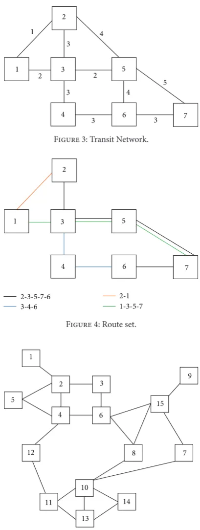
4.3. Fitness Evaluation. During the Fitness evaluation, the fitness value will determine the quality of the solutions and enables them to be compared.Figure 3shows an example of a transit network with the distance (in minutes) stated between two nodes, whereasFigure 4 represents a feasible route set with the number of 4 routes and a maximum of 5 nodes in a route. Notice the difference between the route set and the original transit network where some links from the transit network may be absent in the route set. Therefore, in the fitness evaluation function, every route set will go through Dijkstra’s algorithm [23] to calculate the shortest path of the route set from each source to each destination.

We assume that every passenger would want to travel through the shortest path. However, in a route set, there might be a possibility of having more than one route sharing the same shortest distance. For example, inFigure 4, to travel from node 2 to node 6, the shortest distance is 9 and a passenger may travel through nodes 2-1-3-4-6 or 2-3-4-6. A five-minute penalty is imposed each time a passenger makes

a transfer. Notice that the first route 2-1-3-4-6 requires two transfers with the total travel time of 19 minutes while the second route 2-3-4-6 requires only one transfer making the total travel time of 14 minutes. This clearly shows that the passenger would prefer the shortest distance with less transfer with lesser total travel time.

Another situation may arise where, in some cases, the passengers may able to travel with a lower travel time with less number of transfer(s) or no transfer at all. By using the example above, if passengers take account of the transfer waiting time when choosing their travel path, the travel path of 2-3-5-7-6 can lead to a lower travel time of 13 minutes with no transfer at all. Fan and Mumford [22] justified that when passengers take account of transfer waiting times when choosing their travel path, it gives results that are at least as good (and probably better) as those when assuming passengers ignore transfer waiting times when choosing their travel paths.

4.4. Selection. In every generation, a proportion of pop-ulation will be selected to undergo genetic operations to breed a new generation. Based on the initial investigations on the selection methods between the roulette wheel, rank, probabilistic binary tournament, and the sexual selections, we adopted the probabilistic binary tournament selection proposed by Deb and Goldberg [24] in the GA. First, a pair of individuals are randomly chosen from the population. Next, a probability will decide whether the fitter individual or the less fitter individual will be chosen to be the parent. Both of the individuals are then returned to the population and may be selected again. The process is repeatedly performed until half of the𝑃poppairs of parents have been selected.

4.5. Crossover. In the crossover phase, GA attempts to exchange portions of two parents to generate an offspring. In this study, route crossover inspired by Chakroborty and Dwivedi [2] is proposed where a random route is selected from each parent. Substrings between the chosen routes swap their position between the two parents, rendering two offspring.Table 1 shows an example of the route crossover between two parents. Route 2 from parent 1 crossed with the substrings of route 1 from parent 2 rendering offspring 1 and 2. Due to the highly complex multiconstrained UTRP, route crossover is able to reduce the possibility of getting an infeasible route set by avoiding infeasibility for criteria I in Section 4.2, and at the same time, search for a better solution with a higher fitness value. However, if the two offspring violated criteria II, III, or IV inSection 4.2, instead of replacing the route set, this genetic operator will be repeated by randomly searching for another route from each parent until two feasible offspring are found. Even so, if none of the possibilities are able to produce two feasible offspring, two new parents are then selected to run the route crossover again. This process is repeated until two feasible offspring are found.

(6)

Start

Construct a partial route set using Floyd’s algorithm

Check if a missing node is

found

Check if the1st

route reaches the maximum number of nodes

Add the missing node to the

first position of the route

Check if the missing node directly links

to its neighbor

Check if the route violates

criteria I

Check if the missing node reached the last position of the

route

Remove the missing node from the current position and insert it

into the next position Route set fulfilled

criteria II

End Discard the

route set Check if the route reached the last route of

the route set Check if the next

route reached maximum number of nodes

Yes Yes

Yes

Yes Yes No

No

No No

No

No No

Run Floyd’s

[image:6.600.103.501.64.724.2]

algorithm

(7)

1

2

3

4

5

6 7

1-2-3-5

5-6

4-6-7

(a)

1

2

3

4

5

6 7

1-2-5

4-6-7

4-3-6

(b)

[image:7.600.134.524.63.605.2]

Figure 2: (a) A connected-7-node network. (b) An unconnected-7-node network.

Table 2: Identical-point mutation.

Offspring 2:

(5 6 01 3 4 0 2 3 5 7 0)

Offspring 2:

(5 6 02 3 4 0 1 3 5 7 0)

Chosen node: 3

4.6. Mutation. The mutation operator helps in maintaining the population diversity by avoiding the population from being trapped in the local optimum. In this study, an identical-point mutation operator based on the modified version of route-crossover genetic operator from Ngamchai and Lovell [14] is proposed. In this mutation, a random node that consists of at least two or more identical nodes in the route set is chosen. The two routes that consist of

3 5 4

2

4

3 3 3 1

2 2

1 3 5

[image:7.600.325.530.67.610.2]

4 6 7

Figure 3: Transit Network.

2

1 3 5

4 6 7

2-3-5-7-6

3-4-6

2-1

1-3-5-7

Figure 4: Route set.

2 1

3

5

4 6

7 8

9

10

11 12

13

15

14

Figure 5: Mandl’s Swiss road network.

[image:7.600.70.281.76.504.2] [image:7.600.51.288.568.606.2]

(8)

1

2 3

4 5

6

7 8

9

10 11

12

13 14

15

Route4

(a)

1

2 3

4 5

6

7 8

9

10 11

12

13 14

15

Route6

(b)

1

2 3

4 5

6

7 8

9

10 11

12

13 14

15

Route7

(c)

1

2 3

4 5

6

7 8

9

10 11

12

13 14

15

Route8

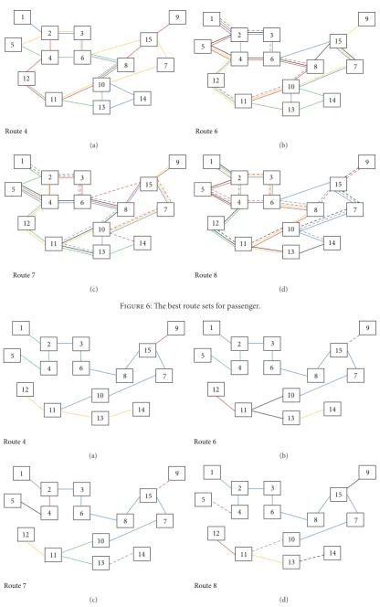
[image:8.600.91.508.62.727.2]

(d)

Figure 6: The best route sets for passenger.

1

2 3

4 5

6

7 8

9

10 11

12

13 14

15

Route4

(a)

1

2 3

4 5

6

7 8

9

10 11

12

13 14

15

Route6

(b)

1

2 3

4 5

6

7 8

9

10 11

12

13 14

15

Route₇

(c)

1

2 3

4 5

6

7 8

9

10 11

12

13 14

15

Route₈

(d)

(9)

10 10.5 11 11.5 12 12.5 13 13.5 14 14.5

60 70 80 90 100 110 120 130 140 150

CP

CO

Nondominated (Pareto Frontier) solutions for case I

(a)

CP

CO

9.5 10 10.5 11 11.5 12 12.5 13 13.5 14

60 80 100 120 140 160 180 200 220 240

Nondominated (Pareto Frontier) solutions for case II

(b)

CP

CO 9.5

10 10.5 11 11.5 12 12.5 13 13.5 14

60 80 100 120 140 160 180 200 220 240 260

Nondominated (Pareto Frontier) solutions for case III

(c)

CP

CO 9.5

10 10.5 11 11.5 12 12.5 13 13.5 14

60 80 100 120 140 160 180 200 220 240 260

Nondominated (Pareto Frontier) solutions for case IV

[image:9.600.66.539.71.408.2]

(d)

Figure 8: Nondominated (Pareto Optimum) solutions for cases I–IV.

replacing it with a new route for criteria I and replacing it with a new route set for criteria II, III, and IV as stated in Section 4.2, the steps in identical-point mutation are repeated with a different random node till a feasible offspring is found. However, if all of the random nodes are unable to produce a feasible offspring, then a new offspring is chosen to perform the mutation. It is important to mention that the mutation operation will only occur to the selected offspring based on the given probability.

4.7. Replacement Strategy. Replacement strategy is executed at the end of each generation where the parent population will be replaced by the offspring population. In the proposed GA, the steady-state replacement strategy is adopted where 10 percent of the best offspring is selected to replace 10 percent of the worst parent in order to keep the population size constant in every generation during implementation. The proposed algorithm terminates when all the individuals in the population converged.

5. Results and Discussions

From the literature review, we discovered that most of the papers have adopted the classical approaches for the

multiobjective UTRP. Pattnaik et al. [6], Tom and Mohan [13], Ngamchai and Lovell [14], and Fan and Machemehl [1] applied the weighted sum method in order to obtain a range of nondominated solutions. Although the weighted sum method is able to provide good solutions, the difficulties of this method are to determine the suitable values for the weights. In addition, it has nonuniformity in the optimal solutions and the inability to search for some Pareto-optimal solutions [25].

In the recent years, Fan et al. [3] and Mumford [18] addressed the UTRP using the evolutionary multi-objective approach. They searched for a set of Pareto-optimal solutions, and the best solution for passenger and operator was chosen from the set. By doing this, decision-making becomes easier and less subjective. In this study, our proposed algorithm will be tested on Mandl’s benchmark data set which contains 15 nodes and 21 links as shown inFigure 5.

(10)

[image:10.600.57.548.88.571.2]

Table 3: The best results obtained by Fan et al. [3].

Case Number of routes Parameters _{results for}The best

passenger

The best routes for passenger

The best results for

operator

The best routes for operator

I 4

𝑑0 90.88 14–13–11–10–8–6–4–5 61.08 2–3–6–8–15–7–10–11

𝑑₁ 8.35 2–4–12–11–10–7–15–9 36.61 15–9

𝑑2 0.77 11–10–8–6–3–2–1 2.31 14–13–11–12

𝑑un 0.00 5–2–3–6–15–7–10 0.00 5–4–2–1

ATT _10.65 _13.88

𝐶𝑂 126 63

II 6

𝑑0 93.19 13–11–10–8–6–3–2–1 66.09 2–3–6–8–15–7–10

𝑑₁ 6.23 7–15–6–3–2–4–5 30.38 9–15

𝑑2 0.58 10–8–6–4–5 3.53 2–1

𝑑un 0.00 13–14–10–11–12–4–2–1 0.00 14–13–11–10

ATT _10.46 _{10–7–15–9} _13.34 _2–4–5

𝐶𝑂 148 12–11–13–14 63 11–12

III 7

𝑑0 92.55 7–15–8 65.64 9–15

𝑑₁ 6.68 14–13–11–12–4–2–3 26.60 11–12

𝑑₂ 0.77 12–11–10–7–15–9 8.61 4–5

𝑑un 0.00 14–10–7–15–6–4–5 0.00 14–13–11

ATT _10.44 _{10–8–6–4–5–2–3} _13.54 _2–4

𝐶𝑂 166 1–2–3–6–8–10–11–13 63 1–2–3–6–8–15–7–10

4–2–1 11–10

IV 8

𝑑₀ 91.33 2–4–12–11–13–14–10 59.92 4–2

𝑑₁ 8.67 12–11–13–14–10–7–15–6 21.37 3–2

𝑑2 0.00 5–2–3–6–8–15–9 18.11 2–1

𝑑un 0.00 1–2–3–6–8–10–11–13 0.00 13–11

ATT 10.45 12–11–13–14–10–8–6–4 13.57 4–5

𝐶𝑂 245 4–6–15–9 63 15–9

5–4–6–8–10–11–13 12–11–10–7–15–8–6–3

12–11–10–7–15–6–3–2 13–14

algorithm on the Mandl’s network for the biobjective UTRP. Therefore, the results provided by Fan et al. [3] and Mumford [18] will be compared with our computational results to assess the efficiency of the proposed algorithm in solving the problem.

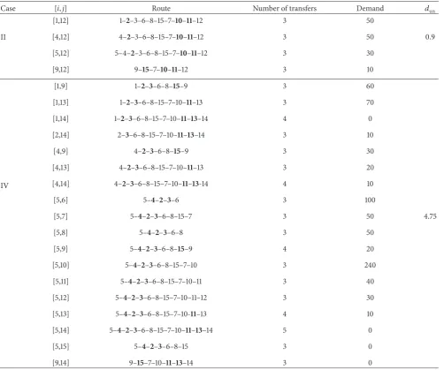
Table 3 contains the results published by Fan et al. [3]. However, we notice that some of the values published do not fit the route sets given. Notice that, from the results published, the percentage of passengers’ demand satisfied with more than two transfers (i.e., demand unsatisfied) in all of the four cases remains constant at the value of 0.00. We found out that, especially from the operators’ point of view, some of the demands of passengers require more than two transfers

to travel from the origin to their destination which leads to a certain percentage of passengers demand unsatisfied. For example,Table 4shows the shortest path of origin node𝑖of passengers that require more than two transfers to reach their destination node 𝑗for cases II and IV from the operators’ point of view. The nodes in bold indicate the station where the passenger needs to make a transfer. According to the best routes published, there is no other possible way that passengers could travel from node𝑖to node𝑗with no more than two transfers. Note that Mandl’s benchmark data set is a symmetric network where[𝑖, 𝑗] = [𝑗, 𝑖]. Therefore, the demand shown in theTable 4represents total demand of[𝑖, 𝑗]

(11)

[image:11.600.52.555.93.512.2]

Table 4: Routes and percentage for passengers’ demand unsatisfied from the operators’ point of view for cases II and IV.

Case [𝑖,𝑗] Route Number of transfers Demand 𝑑_un

II

[1,12] 1–2–3–6–8–15–7–10–11–12 3 50

[4,12] 4–2–3–6–8–15–7–10–11–12 3 50 0.9

[5,12] 5–4–2–3–6–8–15–7–10–11–12 3 30

[9,12] 9–15–7–10–11–12 3 10

IV

[1,9] 1–2–3–6–8–15–9 3 60

[1,13] 1–2–3–6–8–15–7–10–11–13 3 70

[1,14] 1–2–3–6–8–15–7–10–11–13–14 4 0

[2,14] 2–3–6–8–15–7–10–11–13–14 3 10

[4,9] 4–2–3–6–8–15–9 3 30

[4,13] 4–2–3–6–8–15–7–10–11–13 3 20

[4,14] 4–2–3–6–8–15–7–10–11–13-14 4 10

[5,6] 5–4–2–3–6 3 100

[5,7] 5–4–2–3–6–8–15–7 3 50 4.75

[5,8] 5–4–2–3–6–8 3 50

[5,9] 5–4–2–3–6–8–15–9 4 20

[5,10] 5–4–2–3–6–8–15–7–10 3 240

[5,11] 5–4–2–3–6–8–15–7–10–11 3 40

[5,12] 5–4–2–3–6–8–15–7–10–11–12 3 30

[5,13] 5–4–2–3–6–8–15–7–10-11–13 4 10

[5,14] 5–4–2–3–6–8–15–7–10–11–13–14 5 0

[5,15] 5–4–2–3–6–8–15 3 0

[9,14] 9–15–7–10–11–13–14 3 0

Table 5: Computational results for method 1.

Case CPU time (sec) Generation Objective Results

𝑑0 𝑑1 𝑑2 𝑑un ATT 𝐶𝑂

I 67.15 327 Passenger 89.84 9.80 0.36 0.00 10.75 131

Operator 67.68 28.13 4.16 0.03 13.83 67

II 101.00 473 Passenger 92.92 6.53 0.55 0.00 10.47 184

Operator 58.66 32.29 7.65 1.39 14.29 69

III 187.80 790 Passenger 92.02 7.58 0.40 0.00 10.51 194

Operator 52.10 27.48 14.32 6.10 15.58 66

IV 618.86 2361 Passenger 91.70 7.72 0.58 0.00 10.59 212

Operator 50.24 20.65 15.85 13.26 16.59 66

Average 243.70 988 Passenger 91.62 7.91 0.47 0.00 10.58 181

[image:11.600.56.548.545.735.2]

(12)

[image:12.600.51.556.90.279.2]

Table 6: Computational results for method 2.

Case CPU time (sec) Generation Objective Results

𝑑0 𝑑1 𝑑2 𝑑un ATT 𝐶𝑂

I 23.33 116 Passenger 88.53 11.11 0.36 0.00 10.93 126

Operator 72.54 25.27 1.93 0.27 13.14 68

II 41.71 145 Passenger 92.92 7.00 0.08 0.00 10.48 175

Operator 66.05 31.20 2.47 0.28 13.36 69

III 50.64 158 Passenger 93.53 6.28 0.19 0.00 10.43 196

Operator 56.81 36.13 6.31 0.75 14.29 67

IV 55.56 172 Passenger 94.68 5.29 0.03 0.00 10.32 231

Operator 60.99 27.85 8.72 2.44 14.61 66

Average 42.81 148 Passenger 92.42 7.42 0.17 0.00 10.54 182

Operator 64.10 30.11 4.86 0.94 13.85 68

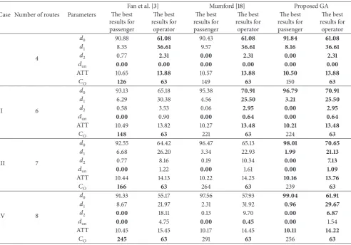
Table 7: Comparison of biobjective results of Mandl’s Swiss road network.

Case Number of routes Parameters

Fan et al. [3] Mumford [18] Proposed GA

The best results for passenger

operator

I 4

𝑑0 90.88 61.08 90.43 61.08 91.84 61.08

𝑑₁ 8.35 36.61 9.57 36.61 8.16 36.61

𝑑₂ 0.77 2.31 0.00 2.31 0.00 2.31

𝑑un 0.00 0.00 0.00 0.00 0.00 0.00

ATT 10.65 13.88 10.57 13.88 10.50 13.88

𝐶_𝑂 126 63 149 63 150 63

II 6

𝑑₀ 93.13 65.18 95.38 70.91 96.79 70.91

𝑑1 6.29 30.38 4.56 25.50 3.21 25.50

𝑑2 0.58 3.53 0.06 2.95 0.00 2.95

𝑑un 0.00 0.90 0.00 0.64 0.00 0.64

ATT 10.49 13.82 10.27 13.48 10.21 13.48

𝐶𝑂 148 63 221 63 224 63

III 7

𝑑0 92.55 64.42 96.47 65.13 98.01 70.65

𝑑₁ 6.68 26.20 3.34 22.93 1.99 21.13

𝑑₂ 0.77 8.16 0.19 10.34 0.00 7.13

𝑑un 0.00 1.22 0.00 1.61 0.00 1.09

ATT 10.44 14.13 10.22 14.25 10.16 13.76

𝐶_𝑂 166 63 264 63 239 63

IV 8

𝑑₀ 91.33 55.17 97.56 57.93 99.04 61.91

𝑑₁ 8.67 21.97 2.31 31.92 0.96 29.67

𝑑2 0.00 18.11 0.13 9.70 0.00 6.87

𝑑un 0.00 4.75 0.00 0.45 0.00 1.54

ATT 10.45 15.45 10.17 14.45 10.11 14.22

𝐶𝑂 245 63 291 63 256 63

note that there will be a 5-minute transfer penalty each time a passenger makes a transfer. Thus, in this case, the added value for𝑑undirectly affects the ATT of passengers as well.

5.1. Experimental Design. As for the computational experi-ment of the proposed algorithm, the population size is set at

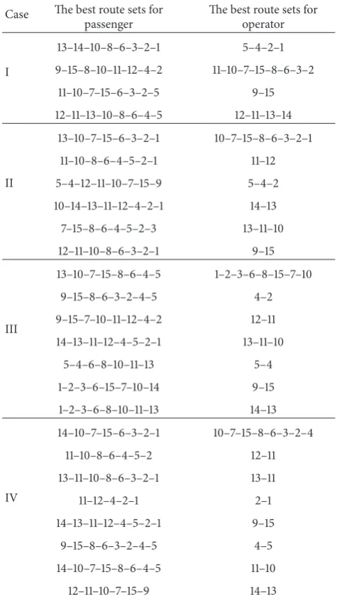
[image:12.600.55.548.307.651.2]

(13)

[image:13.600.49.292.100.528.2]

Table 8: The best route sets for passenger and operator for all four cases.

Case The best route sets for

passenger

The best route sets for operator

I

13–14–10–8–6–3–2–1 5–4–2–1

9–15–8–10–11–12–4–2 11–10–7–15–8–6–3–2

11–10–7–15–6–3–2–5 9–15

12–11–13–10–8–6–4–5 12–11–13–14

II

13–10–7–15–6–3–2–1 10–7–15–8–6–3–2–1

11–10–8–6–4–5–2–1 11–12

5–4–12–11–10–7–15–9 5–4–2

10–14–13–11–12–4–2–1 14–13

7–15–8–6–4–5–2–3 13–11–10

12–11–10–8–6–3–2–1 9–15

III

13–10–7–15–8–6–4–5 1–2–3–6–8–15–7–10

9–15–8–6–3–2–4–5 4–2

9–15–7–10–11–12–4–2 12–11

14–13–11–12–4–5–2–1 13–11–10

5–4–6–8–10–11–13 5–4

1–2–3–6–15–7–10–14 9–15

1–2–3–6–8–10–11–13 14–13

IV

14–10–7–15–6–3–2–1 10–7–15–8–6–3–2–4

11–10–8–6–4–5–2 12–11

13–11–10–8–6–3–2–1 13–11

11–12–4–2–1 2–1

14–13–11–12–4–5–2–1 9–15

9–15–8–6–3–2–4–5 4–5

14–10–7–15–8–6–4–5 11–10

12–11–10–7–15–9 14–13

computer running on Windows 7 with Intel (R) Core 2 Duo CPU 1.3 GHz and 2 GB of RAM.

5.2. sBiobjective Implementation. As mentioned inSection 3, the two objective functions that we are trying to optimize are 𝐶_𝑃 and 𝐶_𝑂. We implement the biobjective UTRP in two different methods separately. Here, we named them as method 1 and method 2. To satisfy the two objective functions𝐶_𝑃and𝐶_𝑂, for Method 1, the algorithm starts with Floyd’s initialization. The algorithm will switch the objective functions in every 10 generations until the solutions have converged. The best nondominated result for each objective will be recorded. As for method 2, instead of switching the objective function in every 10 generations, the objective function will only be switched when the entire population for the first objective (𝐶_𝑃) has converged. Therefore, in method 2,

the algorithm will only switch once and both of the objective functions will start with the same initial population that has been recorded earlier.

To make comparison between the methods, each case in Mandl’s network will be run five times. Five sets of the initial population are previously recorded so that, in each run, both of the methods will be using the same initial population. Tables5and6show average computational results for each case for method 1 and method 2. The last row in each table represents the overall average of all cases. From the results shown, it is undeniable that method 2, shows a better value especially in terms of execution time and the number of generations. The execution time and number of generation for method 1 increase dramatically when the number of route increases. Thus, we decided to use method 2 in our proposed algorithm to solve the biobjective UTRP.

5.3. Comparative Results for Biobjective Mandl’s Swiss Transit Network. As for the final computational experiment, for each case, the proposed GA is performed for 30 runs for statistical significance. 30 nondominated solutions for each of the objective functions will be recorded as the output. In every generation of each run, both of the objectives value are tested to see whether the value improves the best solutions recorded. If yes, it will replace the current best solution. After the population has converged, the nondominated solutions will be returned as output.

As mentioned earlier, the route sets published by Fan et al. [3] do not match the parameters’ value. Thus, inTable 7, we record the corrected results of Fan et al. [3] according to the route sets published. The last two columns show the best parameters’ values obtained for the two objectives based on the proposed GA. The values in bold represent the best results of each parameter.

The 𝐶_𝑃 and 𝐶_𝑂 are always contradicting each other. Therefore, it is reasonable that the lowest𝐶_𝑃will correspond with the highest𝐶_𝑂[3]. InTable 7, from the passengers’ point of view, we obtained a very satisfactory𝐶_𝑃 value with the highest value of𝑑₀reaching 99.04% and the lowest ATT value of 10.11 minutes in case IV. We constantly outperformed the results of [3, 18] in all cases. Nevertheless, the low 𝐶_𝑃 has led to a higher𝐶_𝑂value. From the operators’ point of view, for case I, we obtained the same values as in Fan et al. [3] in all parameters, whereas for cases II, III, and IV, even though we obtained the same value for𝐶_𝑂 as in Fan et al. [3] for all cases, we constantly bettered the values for the rest of the parameters. Similar pattern of results is obtained as compared to Mumford [18]. The percentage for passengers to travel to their destination without any transfer is up to 70.91% and the unsatisfied customer in all cases is not more than 1.54%. The lowest value for the ATT from the operators’ point of view is 13.48 minutes.

(14)

[image:14.600.52.549.89.217.2]

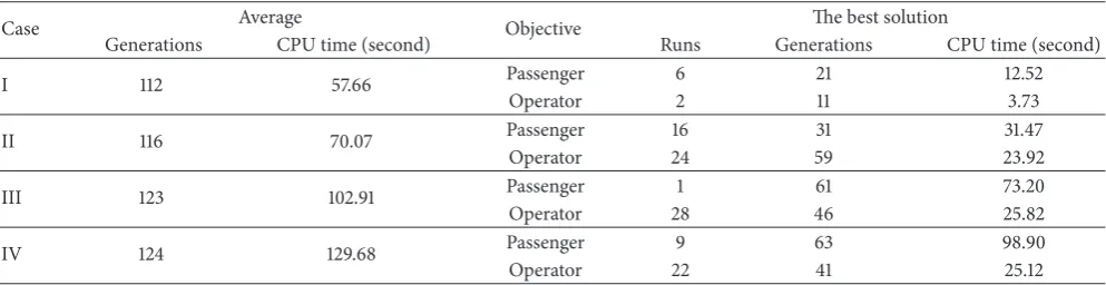
Table 9: The average and the best solutions found in terms of number of generations, number of runs, and CPU time.

Case Average Objective The best solution

Generations CPU time (second) Runs Generations CPU time (second)

I 112 57.66 Passenger 6 21 12.52

Operator 2 11 3.73

II 116 70.07 Passenger 16 31 31.47

Operator 24 59 23.92

III 123 102.91 Passenger 1 61 73.20

IV 124 129.68 Passenger 9 63 98.90

and 57.66 seconds, respectively. The best solution from the passengers’ point of view was obtained on run number 6 at the 21st generation with the CPU time of 12.52 seconds starting from the 6th run. In the operators’ point of view, on the other hand, the best solution is obtained on the 2nd run at the 11th generation with the CPU time of 3.73 seconds. Finally, the 30 nondominated solutions for each of the objective functions from the 30 runs which formed the Pareto Frontier for case I to case IV can be seen inFigure 8. Through the nondominated solutions from the Pareto Frontier, it is up to the decision maker to search for the best suited solution among all the nondominated solutions.

6. Conclusion

In this paper, we solved the biobjective UTRP by looking at the passengers’ and operators’ points of view. The proposed GA for the biobjective UTRP is first being initialized by using Floyd’s initialization. The initial population must satisfy the four feasible criteria in order to generate feasible solutions. Among them, an adding-node procedure is introduced to convert an infeasible solution to a feasible one. Furthermore, route crossover and identical-point mutation are proposed to perform the genetic operations. We executed the biobjective UTRP by switching the objective function after the first objective has converged. The proposed GA is tested on Mandl’s benchmark data set and it has performed better than the previous best published results from the literature in most cases.

References

[1] W. Fan and R. B. Machemehl, “Optimal transit route network design problem with variable transit demand: genetic algorithm

approach,”Journal of Transportation Engineering, vol. 132, no. 1,

pp. 40–51, 2006.

[2] P. Chakroborty and T. Dwivedi, “Optimal route network design

for transit systems using genetic algorithms,”Engineering

Opti-mization, vol. 34, no. 1, pp. 83–100, 2002.

[3] L. Fan, C. L. Mumford, and D. Evans, “A simple multi-objective optimization algorithm for the urban transit routing

problem,” inProceedings of the IEEE Congress on Evolutionary

Computation (CEC ’09), pp. 1–7, Trondheim, Norway, May 2009.

[4] C. A. Coello Coello, “Evolutionary multi-objective

optimiza-tion: a historical view of the field,”IEEE Computational

Intel-ligence Magazine, vol. 1, no. 1, pp. 28–36, 2006.

[5] R. W. Floyd, “Algorithm 97: shortest path,”Communications of

the ACM, vol. 5, no. 6, article 345, 1962.

[6] S. B. Pattnaik, S. Mohan, and V. M. Tom, “Urban bus transit

route network design using genetic algorithm,” Journal of

Transportation Engineering, vol. 124, no. 4, pp. 368–375, 1998. [7] S. Chien, Z. Yang, and E. Hou, “Genetic algorithm approach

for transit route planning and design,”Journal of Transportation

Engineering, vol. 127, no. 3, pp. 200–207, 2001.

[8] M. Bielli, P. Carotenuto, and G. Confessore, “A new approach

for transport network design and optimization,” inProceedings

of the 38th Congress of the European Regional Science Association (ERSA ’98), 1998.

[9] Y. Xiong and J. B. Schneider, “Transportation network design

using a cumulative algorithm and neural network,”

Transporta-tion Research Record, vol. 1364, 1993.

[10] M. Bielli, M. Caramia, and P. Carotenuto, “Genetic algorithms

in bus network optimization,”Transportation Research C, vol.

10, no. 1, pp. 19–34, 2002.

[11] G. Fusco, S. Gori, and M. Petrelli, “A heuristic transit network

design algorithm for medium size towns,” in Proceedings of

the 13th Mini-EURO Conference Handling Uncertainty in the Analysis of Traffic and Transportation Systems, pp. 652–656. [12] M. H. Baaj and H. S. Mahmassani, “Hybrid route generation

heuristic algorithm for the design of transit networks,”

Trans-portation Research C, vol. 3, no. 1, pp. 31–50, 1995.

[13] V. M. Tom and S. Mohan, “Transit route network design using

frequency coded genetic algorithm,”Journal of Transportation

Engineering, vol. 129, no. 2, pp. 186–195, 2003.

[14] S. Ngamchai and D. J. Lovell, “Optimal time transfer in bus

transit route network design using a genetic algorithm,”Journal

of Transportation Engineering, vol. 129, no. 5, pp. 510–521, 2003. [15] C. L. Valenzuela, “A simple evolutionary algorithm for

multi-objective optimization (SEAMO),” inProceedings of the

Congress on Evolutionary Computation (CEC ’02), pp. 717–722, Honolulu, Hawaii, USA, 2002.

[16] C. L. Mumford, “Simple population replacement strategies for

a steady-state multi-objective evolutionary algorithm,”Lecture

Notes in Computer Science, vol. 3102, pp. 1389–1400, 2004. [17] W. Y. Szeto and Y. Wu, “A simultaneous bus route design

and frequency setting problem for Tin Shui Wai, Hong Kong,”

(15)

[18] C. L. Mumford, “New heuristic and evolutionary operators for

the multi-objective urban transit routing problem,” in IEEE

Congress on Evolutionary Computation (CEC ’13), pp. 939–946, 2013.

[19] C. Mandl, Applied Network Optimization, Academic Press,

London, UK, 1979.

[20] M. H. Baaj and H. S. Mahmassani, “AI-based approach for

transit route system planning and design,”Journal of Advanced

Transportation, vol. 25, no. 2, pp. 187–210, 1991.

[21] F. A. Kidwai,Optimal Design of Bus Transit Network: A Genetic

Algorithm based Approach, Indian Institute of Technology, Kanpur, India, 1998.

[22] L. Fan and C. L. Mumford, “A metaheuristic approach to the

urban transit routing problem,”Journal of Heuristics, vol. 16, no.

3, pp. 353–372, 2010.

[23] E. W. Dijkstra, “A note on two problems in connexion with

graphs,”Numerische Mathematik, vol. 1, no. 1, pp. 269–271, 1959.

[24] K. Deb and D. E. Goldberg, “An investigation of niche and

species formation in genetic function optimization,” in

Proceed-ings of the 3rd International Conference on Genetic Algorithms, pp. 42–50, 1989.

[25] K. Deb,Multi-Objective Optimization Using Evolutionary

(16)

Submit your manuscripts at

http://www.hindawi.com

Hindawi Publishing Corporation

http://www.hindawi.com Volume 2014

Mathematics

Journal of

Hindawi Publishing Corporation http://www.hindawi.com

Differential Equations

International Journal of

Volume 2014

Applied MathematicsJournal of

Mathematical PhysicsAdvances in

Complex Analysis

Journal of

Optimization

Journal of

Combinatorics

International Journal of

Journal of

Function Spaces

Abstract and Applied Analysis

International Journal of Mathematics and Mathematical Sciences

Hindawi Publishing Corporation http://www.hindawi.com Volume 2014

The Scientific

World Journal

Discrete Dynamics in Nature and Society

Discrete Mathematics

Journal of

Genetic algorithm for biobjective urban transit routing problem

Research Article