Advance Access publication 2016 September 19
The effect of a wider initial separation on common envelope binary
interaction simulations
Roberto Iaconi,
1‹Thomas Reichardt,
1Jan Staff,
1,2Orsola De Marco,
1Jean-Claude Passy,
3Daniel Price,
4James Wurster
4,5and Falk Herwig
61Department of Physics and Astronomy, Macquarie University, Sydney, NSW 2109, Australia 2Department of Astronomy, the University of Florida, Gainesville, FL 32611, USA
3Argelander Institute f¨ur Astronomie, Bonn Universit¨at, D-53121, Bonn, Germany
4Monash Centre for Astrophysics and School of Physics and Astronomy, Monash University, Clayton, VIC 3800, Australia 5Astrophysics Group, School of Physics, University of Exeter, Stocker Road, Exeter EX4 4QL, UK
6Department of Physics and Astronomy, University of Victoria, Victoria, BC V8P 5C2, Canada
Accepted 2016 September 15. Received 2016 September 14; in original form 2016 March 2
A B S T R A C T
We present hydrodynamic simulations of the common envelope binary interaction between a giant star and a compact companion carried out with the adaptive mesh refinement code ENZOand the smooth particle hydrodynamics code PHANTOM. These simulations mimic the parameters of one of the simulations by Passy et al. but assess the impact of a larger, more realistic initial orbital separation on the simulation outcome. We conclude that for both codes the post-common envelope separation is somewhat larger and the amount of unbound mass slightly greater when the initial separation is wide enough that the giant does not yet overflow or just overflows its Roche lobe.PHANTOMhas been adapted to the common envelope problem here for the first time and a full comparison withENZOis presented, including an investigation of convergence as well as energy and angular momentum conservation. We also set our simulations in the context of past simulations. This comparison reveals that it is the expansion of the giant before rapid in-spiral and not spinning up of the star that causes a larger final separation. We also suggest that the large range in unbound mass for different simulations is difficult to explain and may have something to do with simulations that are not fully converged.
Key words: hydrodynamics – methods: numerical – stars: AGB and post-AGB – binaries: close – stars: evolution.
1 I N T R O D U C T I O N
The common envelope (CE) interaction is a short phase of the interaction between two stars in a binary system characterized by the dense cores of the two objects orbiting inside their merged
envelopes. It was first described by Paczynski (1976), but see also
Ivanova et al. (2013) and references therein. During this phase,
orbital energy and angular momentum are transferred to the gas of the envelope, which can become unbound from the potential well of the system, leaving behind a close binary. In cases when the envelope is not unbound, a merger results.
The CE phase is thought to be the main evolutionary channel that leads to all the evolved compact binaries. Post-CE compact binaries can eventually merge on longer time-scales. In addition to compact binaries, mergers inside the CE can take place. In this case energy and angular momentum from the orbit are entirely dissipated
E-mail:[email protected]
into the envelope, which may be not entirely ejected. Objects and phenomena resulting from these scenarios include Type Ia super-novae, low- and high-mass X-ray binaries, double neutron star and double black holes. A full physical description of all binary interac-tion scenarios, including the CE phase, is essential in constructing state-of-the-art stellar population synthesis models to understand the rates at which compact binaries and mergers form (see Toonen
et al.2014and references therein for an exhaustive review of both
binary evolution scenarios including CE and their rates). Hydrody-namics simulations are an essential tool to investigate the physics of the CE phase and determine the outcome of CE interactions as a function of initial binary parameters.
Past efforts have tried to reproduce numerically CE interactions
with different codes (e.g. Rasio & Livio1996; Sandquist et al.1998;
Sandquist, Taam & Burkert2000; Passy et al.2012; Ricker & Taam
2012; Nandez, Ivanova & Lombardi2014), but failed to reproduce
the post-CE systems observed. Primarily, simulations fail to unbind the entire envelope. While the envelope is lifted away from the in-spiralling binary, the majority of it is not unbound (e.g. Passy
C
2016 The Authors Published by Oxford University Press on behalf of the Royal Astronomical Society
et al.2012). Recently Ivanova, Justham & Podsiadlowski (2015)
and Nandez, Ivanova & Lombardi (2015) reported that adding
re-combination energy in their simulations achieves the unbinding of the envelope under at least a certain combination of parameters.
Current simulations are limited in one way or another. The range of physical phenomena taken into consideration is still very limited (e.g. the effect of magnetic fields is possibly important; Reg˝os &
Tout1995; Nordhaus, Blackman & Frank2007; Tocknell, De Marco
& Wardle2014; Ohlmann et al. 2016b). In addition, the initial
conditions of the simulations are often non-physical. For example, many simulations start with the companion on or close to the surface
of the primary (Passy et al.2012; Ricker & Taam2012). Despite
the growing number of simulations, binary parameter space is still sparsely covered. Additionally, different numerical techniques are
used, e.g. unigrid (Passy et al.2012), adaptive mesh refinement
(AMR; Ricker & Taam2012), smoothed particle hydrodynamics
(SPH; Nandez et al.2014) and unstructured mesh (Ohlmann et al.
2016a), but only seldom benchmark comparisons exist (e.g. Passy
et al.2012). Finally, the resolution of the simulations is always
relatively low (but see the improvement in the latest simulations by
Ohlmann et al.2016a) and the available convergence tests are never
exhaustive enough, due to the substantial computational demands of these simulations, to convince that resolution does not play a part in the outcome of the simulations. Thus, determining the effect that individual aspects of the simulations have on the results is a way to provide insight into which of the effects has the largest impact on the simulation’s outcome.
Here we analyse the effect of the initial orbital separation on the final outcome of the CE simulations by carrying out a set of simula-tions that parallel one of the simulasimula-tions carried out by Passy et al.
(2012, hereafterP12), where a 0.88 Mred giant branch (RGB)
star interacts with its 0.6 Mcompact companion. In their
simu-lation, the companion was initially placed near the surface of the giant. In one of our simulations we place instead the companion at the approximate largest distance from which an orbiting companion is likely to be brought into Roche lobe contact with a giant. It is expected that prior to the start of the CE in-spiral phase, tidal forces will redistribute orbital energy and angular momentum from the or-bit to the primary. Eventually the primary would overflow its Roche lobe and start mass transfer to the companion, finally resulting in the fast CE in-spiral. These phases are expected to induce enve-lope rotation and expansion, changing the overall distribution of the envelope and lowering its binding energy. The envelope would be lighter and easier to unbind, but the overall strength of the
gravi-tational drag (Ostriker1999) may be smaller because of relatively
lower densities and smaller velocity contrasts. It is therefore not clear a priori what effect a larger initial separation would have on the simulation.
The effect of a rotating giant on the CE outcome could only
be gauged by Sandquist et al. (1998) who carried out side-by-side
simulations with rotating and non-rotating giants and determined
that the outcome does not vary much. Rasio & Livio (1996), Ricker
& Taam (2012) and Ohlmann et al. (2016a) all used a rotating
giant, but did not compare their results with a non-rotating case. In
addition, while Rasio & Livio (1996) stabilized the rotating giant,
none of the other studies did, introducing doubts as to the impact of the giant rotational expansion on the results. Finally, all simulations started at a separation such that the giant was already overflowing its Roche lobe and thus could not gauge the effects of a more gradual expansion of the giant envelope.
In line with the work ofP12we carry out our simulations with
grid (in AMR mode) and SPH codes. In so doing we continue to
compare different numerical techniques while making the most of
what each has to offer. The SPH code we use,PHANTOM(Lodato
& Price2010; Price & Federrath2010), has never been used for
CE interaction simulations before, hence this work serves also to
introducePHANTOMto this problem.
This paper is organized as follows. In Section 2 we explain the simulations’ set-up. In Section 3 we analyse the outputs of our simulations, focusing on the evolution of the orbital separation in Section 3.1, the distribution of the envelope in Sections 3.2 and 3.3, the gravitational drag during the interaction in Section 3.4 and the energetics and the numerical behaviour of the codes in Section 3.5. In Section 4 we set our results in the context of all previous simulations while in Section 5 we conclude.
2 S I M U L AT I O N S S E T- U P
We use two different codes to simulate our physical problem:ENZO
(O’Shea et al. 2004; Bryan et al. 2014), an Eulerian code with
AMR andPHANTOM(Lodato & Price2010; Price & Federrath2010)
an SPH code.
ENZOis a parallel 3D hydrodynamic code including self-gravity,
originally developed for cosmological simulations, which has been
adapted for CE simulations as described inP12.ENZOalready had
AMR capabilities whenP12performed their simulation, but they
were not available for CE simulation. Therefore, they performed their simulations with a static, uniform grid. However, given the
most recent updates applied toENZO(Passy & Bryan2014), we used
the AMR capabilities of the code, which guarantee better resolution where needed and a better usage of computational resources.
Our simulation has been run with a cubic box of 863 R =4 au
on a side and a coarse grid resolution of 128 cells per side. We adopt two levels of refinement with a refinement factor of 2 (i.e. when a cell is refined it is divided by two along each dimension),
in this way the smaller cell size is 1.68 R, as was the case in the
2563simulations ofP12. The refinement criterion is based on cell
gas density. Cell densities above 1.38×10⁻⁸g cm−3dictate a cell
division. AdditionallyENZOadaptively de-refines the zones where
a cell and its surrounding region no longer satisfy the refinement criterion. For our choice of the smoothing length (see below), two levels of refinement are the minimum to obtain a stable giant model with the best possible energy conservation.
Ricker & Taam (2012), who carried out the only other CE
sim-ulations adopting an Eulerian AMR approach, use a computational
domain of 575 R =2.7 au with nine levels of refinement,
ob-taining a smallest cell length of 0.29 R, approximately six times
smaller than the value we obtain in this work.
As we will explain in Sections 2.1 and 2.2, we use point masses, interacting only gravitationally with both gas and other particles, to model the primary core and the companion. This point mass
po-tential is smoothed according to the prescription of Ruffert (1993).
To ensure reasonable energy conservation, our smoothing length is equal to three times the smallest cell size, as this was found to be
the optimal value by Staff et al. (2016a), who monitored the energy
conservation in their CEENZOsimulations as a function of
smooth-ing length. A smoothsmooth-ing length of 1.5 times the smallest cell size, as
used by Sandquist et al. (1998) andP12, results in a non-negligible
energy non-conservation in our simulations for this particular case. Increasing the smoothing length reduces the strength of the gravity over a larger volume around the point masses. Our choice for the
smoothing length (3×[smallest cell size]5 R) yields a radius
inside which gravity is smoothed that is double that ofP12’s 2563
simulations.
PHANTOMis a shared memory (OpenMP) parallelized, 3D SPH
code.PHANTOM was originally designed to model star formation,
but it has been expanded to simulate different types of
astrophys-ical problems because of its modularity. We modified PHANTOM,
allowing the code to setup 3D stellar models based on 1D stellar evolution codes radial profiles and then to create binary systems for CE simulations.
OurPHANTOMsimulations have been run with variable total num-bers of particles to test for convergence (see Section 2.3). However, the main simulations we use for our results have been carried out
with one million particles. Similarly to theENZOprocedure, we use
point masses (called sink particles in thePHANTOMnomenclature),
interacting only gravitationally with both gas and SPH particles, to model the primary core and the companion (see Sections 2.1 and 2.2). Both core and companion particles were given a softening
length1of 3 R
, irrespective of the total number of particles used.
The methodology followed to simulate our CE interaction con-sists of two main phases and is described in the following sections.
2.1 Single star set-up and stabilization
As in P12we model our binary system as an RGB primary and
a smaller companion with comparable mass, identifiable with a main-sequence star or a compact object such as a white dwarf. The resolution is not sufficient to resolve the primary’s core, or the companion, so we model them as dimensionless point masses. The
companion mass isM2=0.6 M(this choice will be discussed in
Section 2.2). The primary star is an extended object whose envelope
is well resolved. We use the same initial model as inP12: a star with
an initial mass of 1 M evolved to the RGB with the 1D stellar
evolution codeEVOL(Herwig2000). At this stage of the evolution,
the star has a radius ofR1=83 R, a total mass ofM1=0.88 M
and a core mass ofMc=0.392 M.
The relevantENZOphysical quantities are interpolated from the
1D model to the 3D domain. Because of the limited resolution of the 3D code, the interpolation process results in a mass deficit that coincides almost exactly with the mass of the core. The addition of a point mass representing the missing mass therefore completes the stellar structure. Moreover, because of the limited resolution, the surface of the star is poorly matched to the steep gradients typical of stellar atmospheres, therefore the part of the simulation box not occupied by the star is filled by low-density medium with
a density equal to 10−4 times the density of the surface layer of
the primary. To match the pressure of the stellar atmosphere this
medium has a high temperature (108 K). However, the stellar
model is not in perfect hydrostatic equilibrium in the grid due to the
higher resolution adopted byEVOLand its more realistic equation of
state that takes microphysics into account, whileENZOhas an ideal
gas equation of state withγ = 53. The primary therefore has to be
stabilized by damping at each time step the velocities that develop in the grid. This stabilization is carried out for 10 dynamical times. The stability of the model in the new grid is then verified by letting the simulation run without damping for 10 additional dynamical times, where our RGB star dynamical time is 21 d.
At the end of this process the initial 3D stellar model is relaxed
with respect to the 1D model as showed in Fig.1(upper panel). The
sharp density jump at the edge of the star has been smoothed by the
1The softening length in
PHANTOMis equivalent to the smoothing length
inENZO.PHANTOMreserves the term ‘smoothing length’ for the size of the
[image:3.595.306.548.53.445.2]smoothing kernel, such that each SPH particle has a smoothing length.
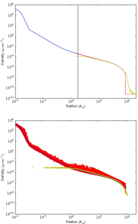
Figure 1. Upper panel: radial density profiles of the primary RGB star used in ourENZOsimulation, calculated with the 1DEVOLcode (blue), after mapping it in theENZOcomputational domain but before the stabilization process (red) and after stabilization (yellow). The change in slope at a radius of 3×10⁻²R
marks the core-envelope boundary of the 1D model, while the vertical line shows the size of anENZOcell at the deepest level of refinement. Lower panel: same as the top panel, but for thePHANTOMcode using 2.3 million particles. Note that while forENZOwe perform a radial average, showing a single density value at each radius, forPHANTOMwe plot the density of all the SPH particles at a given radius. As a result the red curve is not simply a line. The lowest density in thePHANTOMsimulation is
larger than forENZObecause of the lack of a low-density ‘vacuum’.
stabilization process, and the star is now slightly larger. The contour
of density of 10−11g cm−3has a radius 100 R
. The central density
is also slightly reduced, but overall the original structure of the star is mostly preserved.
To verify the stability of the model more quantitatively than
pre-viously done (Sandquist et al.1998;P12; Ricker & Taam2012),
the velocities that develop have been compared to global and local velocity scales, such as the local sound speed and the dynamical
velocity,vdyn,1=R1/tdyn,1R1(Gρ1)
1
2, wheretdyn,1 is the
dy-namical time of the primary,Gis the gravitational constant and
ρ1is the average density of the star. Additionally, we also
com-pare the gas velocities in the frame of reference of the primary to the orbital velocities of the binary system in the frame of reference
MNRAS464,4028–4044 (2017)
of the centre of mass (see Section 2.2). At each step during the relaxation at most 7 per cent of the cells had velocities exceed-ing the lowest of the velocity limits discussed above. Hence we expect the contamination of the CE interaction by the spurious mo-tions of the primary envelope to be negligible.
InPHANTOMwe map the same 1D stellar model, but in this case the SPH particles are distributed so as to reproduce the entire stellar mass distribution, inclusive of the core. This generates a very high particle density at the location of the core that would slow down the simulation excessively. We therefore approximate the core of the giant using a sink particle set-up to accrete all SPH particles
within a radius of 0.03 R. This quickly generated a ‘core’ with
the correct mass (Mc=0.392 M). Note that the number of particles
mentioned for all thePHANTOMsimulations in the following sections
is the actual number of particles after the accretion process (e.g.
the convergence test using 2.3×10⁶particles described in Section
2.3 was actually initialized with4×106particles). The giant was
then damped and stabilized as was done forENZO. The profiles of
the star as mapped inPHANTOMare shown in Fig.1(lower panel).
2.2 Binary system set-up
The companion has a massM2=0.6 Mfor both theENZOand the
PHANTOMsimulations, selected among those simulated byP12, also
based on the fact that their 0.6 Mcompanion simulations were
converged for the coarse grid resolutions we are using. However, theENZOandPHANTOMsimulations differ for the initial separation of the binary.
InENZOthe orbital separation was the largest that would result in
the evolution of the orbital elements and eventually in a CE:a=
300 R(corresponding to a period of 496 d=1.36 yr). This value
also corresponds to the approximate maximum orbital separation from which a tidal capture of the companion may take place within the evolution of a star similar to our primary: Madappatt, De Marco
& Villaver (2016) show that a 1.5 Mstar grows to have a maximum
RGB radius of 130 Rand can engulf a 0.15 Mcompanion that
orbits as far as 2.5 times that radius. Hence it is reasonable that our
star with a radius of∼100 Rcan succeed in capturing tidally a
companion that is as far as approximately 300 R. The system was
placed in circular orbit, where we gave the RGB star a Keplerian
velocity v1 12.4 km s−1 and the companion point particle a
velocityv218.2 km s−1, with the point mass core of the primary
coinciding with the centre of the box.
In our simulation the primary is driven into Roche lobe
con-tact (the Roche lobe radius of the primary is 124 R at an
or-bital separation of 300 R, using the approximation of Eggleton
1983, but noting it to be valid in the case of synchronized orbits,
which is not our case) and eventually a CE interaction by the
pre-contact tidal interactions in a relatively short time-scale (1.5 yr, see
Section 3.1), much shorter than realistic tidal interaction time-scales. Tidal interaction simulations performed by Madappatt et al.
(2016) show in fact that the time-scale for the engulfment of a
0.15 M companion by a 1.5 M primary initially orbiting at
300 Ris of the order of 100 000 yr. Although this system is
slightly different from the one simulated here, a tidal interaction time not too dissimilar is expected in our case. The reason for this differ-ence is that the strength of the interaction is sensitive to departures of the stellar envelope distribution from spherical. Inserting the com-panion in the computational domain generates a small distortion of the primary’s envelope resulting in a set of oscillations, which exert a relatively strong tidal force. Paradoxically, this larger than average tide results in shortening of the orbital separation within reasonable
computational times, something that would not be so if the tide were better reproduced. For more discussion on this topic see Section 3.3. We do not apply any initial rotation to the primary. However, we achieve a spinning star by spin–orbit interaction. This means that the total angular momentum in the system, which is increas-ingly transferred from the orbit to the envelope of the giant, is approximately that which would be expected for this system (see Section 3.5).
We carried out two mainPHANTOMsimulations. The first one has
similar parameters to that carried out byP12 with a companion
mass of 0.6 Mand is used as a verification step to ensure that
PHANTOMperforms similarly to the other codes we have used. This simulation’s outcomes were compared directly with the SPH sim-ulation ‘SPH2’, which in that study was carried out with the SPH codeSNSPH(Fryer, Rockefeller & Warren2006) using 500 000 SPH particles. Additionally, for this binary configuration, we carried out a resolution test, described in Section 2.3.
The secondPHANTOMsimulation has a larger initial separation,
to corroborate whether a larger initial separation promotes a wider
final separation. The initial separation we use in this case is 218 R,
the distance at which the primary fills its Roche lobe. Ideally we
would have used a larger separation of 300 R, like for theENZO
simulation discussed above. However, the orbital evolution of a PHANTOMsimulation with an initial separation of 300 Rwas too slow to reach the CE phase in reasonable computational times. This is due to the stability of SPH simulations to surface deformations
(Springel2010; see also our discussion in Section 3.3 and Fig.10).
Rasio & Livio (1996) and Nandez et al. (2014,2015) stabilize
their giants in the corotating frame of the binary, while slowly decreasing the orbital separation to the desired value (for a more
detailed description see Rasio & Livio1996). We do not apply
this additional stabilization in our simulations. Similarly to us, the
simulations of Sandquist et al. (1998,2000) and Ricker & Taam
(2012), all starting with a separation larger than the radius of the
primary (see Table1), did not stabilize their giants in the corotating
frame.
2.3 PHANTOM convergence test
SincePHANTOMwas used here for the first time to simulate a CE
interaction, we carried out a convergence test to better understand the behaviour of the code at different resolutions. We used three resolutions: 23 000, 230 000 and 2.3 million particles, and we show
the evolution of the orbital separation in the three cases in Fig.2.
The factor of 10 difference between the resolutions is just larger than the minimum resolution step needed for such a test. While this test shows that we have not yet achieved formal convergence, the change in orbital evolution with resolution is much smaller between the higher two resolutions than between the lower two, indicating converging behaviour.
3 R E S U LT S
3.1 Orbital separation
For ourENZOsimulation the separation between the point masses
as a function of time and the orbital decay rate are shown in
Fig. 3. To determine the time when the mass transfer phase
be-gins, we calculated the Roche lobe surface around the primary using the total potential field computed in the simulation. Then, we checked whether the cells contained within the primary’s Roche lobe, including the first cell near the inner Lagrangian point in the
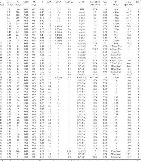
Table 1. A comparison of initial conditions and final outcomes of previous CE simulations that included at least one giant star.
M1 M1, c R1 Giant M2 q ai/R1 /ωa R1/R1, RL Codeb Resolution τrunc adf MUnbe Ref.f
(M) (M) (R) (M) (part./R) (d) (R) (per cent)
4 0.7 66 RGB 0.7 0.18 1.6 1(y) 1.3 SPH 500k 124 1(e) 10(?) 1
3 0.7 200 AGB 0.4 0.13 1.4 1(n) 1.3 n-grid 2.2 800 4.4(a) 41(?) 2
3 0.7 200 AGB 0.4 0.13 1.4 0 1.3 n-grid 2.2 800 4.7(a) 46(?) 2
5 1.0 200 AGB 0.4 0.08 1.4 1(n) 1.2 n-grid 2.2 800 4.4(a) 21(?) 2
5 1.0 200 AGB 0.6 0.12 1.4 1(n) 1.3 n-grid 2.2 800 4.8(a) 45(?) 2
5 0.94 354 AGB 0.6 0.12 1.5 0 1.2 n-grid 2.2 800 8.9(a) 46(?) 2
2 0.335 44 RGB 0.2 0.1 1.3 0.14(n) 3.7 n-grid 2.2 1050 2.1(a) 3(?) 3
1 0.28 22 RGB 0.35 0.35 1.3 0.23(n) 2.6 n-grid 2.2 1050 1.8(a) 10(?) 3
1 0.45 243 RGB 0.35 0.35 1.3 0.24(n) 2.6 n-grid 2.2 1050 21(a) 11(?) 3
1 0.45 221 RGB 0.1 0.1 1.3 0.14(n) 3.7 n-grid 2.2 1050 33(a) 4(?) 3
2 0.45 177 RGB 0.35 0.18 1.3 0.18(n) 3.2 n-grid 2.2 1050 19(a) 6(?) 3
1 0.28 18 RGB 0.45 0.45 1.3 0.26(n) 2.5 n-grid 2.2 1050 2.4(a) 14(?) 3
1.05 0.36 31 RGB 0.6 0.57 2.0 0.95(n) 1.2 a-grid(F) 0.29 60 9(e) 26(t) 4
0.88 0.39 85 RGB 0.1 0.11 1.0 0 1.8 u-grid(E) 1.7 1000 5.7(a)/4.2(e) – 5
0.88 0.39 85 RGB 0.15 0.17 1.0 0 1.9 u-grid (E)1.7 1000 6.9(a)/4.7(e) – 5
0.88 0.39 85 RGB 0.3 0.34 1.0 0 2.1 u-grid(E) 1.7 1000 11(a)/9.0(e) – 5
0.88 0.39 85 RGB 0.6 0.68 1.0 0 2.4 u-grid(E) 1.7 1000 19(a)/16(e) – 5
0.88 0.39 85 RGB 0.9 1.02 1.0 0 2.6 u-grid(E) 1.7 1000 26(a)/22(e) – 5
0.88 0.39 83 RGB 0.1 0.11 1.0 0 1.8 SPH(S) 500k 1050 6.1(a)/5.7(e) 2(t) 5
0.88 0.39 83 RGB 0.15 0.17 1.0 0 1.9 SPH(S) 500k 950 7.3(a)/7.8(e) 6(t) 5
0.88 0.39 83 RGB 0.3 0.34 1.0 0 2.1 SPH(S) 500k 750 11(a)/10(e) 8(t) 5
0.88 0.39 83 RGB 0.6 0.68 1.0 0 2.4 SPH(S) 500k 950 21(a)/18(e) 10(t) 5
0.88 0.39 83 RGB 0.9 1.02 1.0 0 2.6 SPH(S) 500k 600 27(a)/25(e) 10(t) 5
1.50 0.32 26g RGB 0.36 0.24 2.0 0 1.0 SPH(SM) 200k (?) 0.91(e) 100(r)h 6
1.98 0.38 49 RGB 0.99 0.5 1.0 0.95(n) 2.3 m-mesh(A) 0.07–0.01 120 4.9(e) 8(t) 7
1.20 0.32 29 RGB 0.32 0.27 2.0 0 1 SPH(SM) 100k 2000 1.4 100 8
1.20 0.32 29 RGB 0.36 0.30 2.1 0 1 SPH(SM) 100k 2000 1.5 100 8
1.20 0.32 29 RGB 0.40 0.33 2.1 0 1 SPH(SM) 100k 2000 1.4 100 8
1.40 0.32 28 RGB 0.32 0.23 2.0 0 1 SPH(SM) 100k 2000 1.1 100 8
1.40 0.32 28 RGB 0.36 0.26 2.0 0 1 SPH(SM) 100k 2000 1.1 100 8
1.40 0.32 28 RGB 0.40 0.29 2.0 0 1 SPH(SM) 100k 2000 1.2 100 8
1.60 0.32 26 RGB 0.32 0.20 1.9 0 1 SPH(SM) 100k 2000 0.87 100 8
1.60 0.32 26 RGB 0.36 0.23 2.0 0 1 SPH(SM) 100k 2000 0.91 100 8
1.60 0.32 31 RGB 0.36 0.23 1.6 1(y) 1 SPH(SM) 100k 2000 0.93 100 8
1.60 0.32 26 RGB 0.40 0.25 2.0 0 1 SPH(SM) 100k 2000 0.96 100 8
1.80 0.32 16 RGB 0.32 0.18 1.9 0 1 SPH(SM) 100k 2000 0.43 100 8
1.80 0.32 16 RGB 0.36 0.20 1.9 0 1 SPH(SM) 100k 2000 0.48 100 8
1.80 0.32 16 RGB 0.40 0.22 2.0 0 1 SPH(SM) 100k 2000 0.53 100 8
1.18 0.36 60 RGB 0.32 0.27 2.0 0 1 SPH(SM) 100k 2000 3.2 100 8
1.18 0.36 60 RGB 0.36 0.31 2.1 0 1 SPH(SM) 100k 2000 3.7 100 8
1.18 0.36 60 RGB 0.40 0.34 2.1 0 1 SPH(SM) 100k 2000 3.5 100 8
1.38 0.36 57 RGB 0.32 0.23 2.0 0 1 SPH(SM) 100k 2000 2.5 100 8
1.38 0.36 57 RGB 0.36 0.26 2.0 0 1 SPH(SM) 100k 2000 2.8 100 8
1.38 0.36 57 RGB 0.40 0.29 2.0 0 1 SPH(SM) 100k 2000 3.0 100 8
1.59 0.36 50 RGB 0.32 0.20 1.9 0 1 SPH(SM) 100k 2000 1.7 100 8
1.59 0.36 50 RGB 0.36 0.23 2.0 0 1 SPH(SM) 100k 2000 1.8 100 8
1.59 0.36 50 RGB 0.40 0.25 2.0 0 1 SPH(SM) 100k 2000 2.1 100 8
1.80 0.36 41 RGB 0.32 0.18 1.9 0 1 SPH(SM) 100k 2000 1.2 100 8
1.80 0.36 41 RGB 0.36 0.20 1.9 0 1 SPH(SM) 100k 2000 1.3 100 8
1.80 0.36 41 RGB 0.40 0.22 2.0 0 1 SPH(SM) 100k 2000 1.4 100 8
0.88 0.39 100 RGB 0.6 0.68 3 0 0.81 a-grid(E) 1.7 2000 36(a)/20(e) 16(t) 9
0.88 0.39 93 RGB 0.6 0.68 1.1 0 2.2 SPH(P) 1m 1850 21(a)/16(e) 13(t) 9
0.88 0.39 91 RGB 0.6 0.68 2.4 0 1.0 SPH(P) 300k 5050 29(a)/22(e) 16(t) 9
aStellar spin frequency as a function of orbital frequency, with an indication of whether the star was stabilized in its rotating configuration (y) or not (n) before
the start of the simulation.
bSPH: smoothed particle hydrodynamics; u-grid: uniform, static grid; n-grid: static nested grids; m-mesh: moving mesh; a-grid: adaptive mesh refinement grid;
F:FLASH; E:ENZO; S:SNSPH; P:PHANTOM; SM:STARSMASHER; A:AREPO.
cInformation not provided (?).
dRounded to two significant figures, calculated either at the end of the simulation (e) or at a time defined by the formula in Section 3.1 (a). eCalculated by including thermal energy (t), not including thermal energy (k), information not provided (?) or including recombination energy (r).
f1: Rasio & Livio (1996); 2: Sandquist et al. (1998); 3: Sandquist et al. (2000); 4: Ricker & Taam (2012); 5: Passy et al. (2012); 6: Nandez et al. (2015);
7: Ohlmann et al. (2016a); 8: Nandez & Ivanova (2016); 9: this work.
gThis is the Roche lobe radius also corresponding to the SPH radius in their simulation.
hNote that the same simulation run without recombination energy unbinds 50 per cent of the envelope, although the authors of that simulations do not present
data to illustrate their statement.
MNRAS464,4028–4044 (2017)
Figure 2. Evolution of the separation,a, between the two particles rep-resenting the core of the primary and the companion, used to show the convergence for thePHANTOMcode. The simulation reproduces the one from
P12with the same companion’s mass as this work (M2=0.6 M). The
number of SPH particles used is 2.3×10⁴(blue), 2.3×10⁵(red) and 2.3×
106(yellow). The inset shows a 10×zoom on the end of the rapid in-spiral
phase.
companion’s Roche lobe, have a density greater than the vacuum’s
density (6.93×10⁻¹²g cm−3). Computed in this way, the beginning
of the contact phase takes place after about 547 d=1.5 yr from
the beginning of the simulation. During this pre-contact phase, the
orbital separation has been reduced from 300 to 265 R, at which
point the primary’s Roche lobe radius is 108 R, similar to the
stellar radius at the start of the simulation.
The mass transfer phase lasts until the companion is engulfed in the envelope of the primary, at which point the rapid in-spiral phase begins. We define the start of the rapid in-spiral phase as the time when the equipotential surface passing through the outer
Lagrangian pointL2has a density greater than the vacuum’s density
in each of its cells. This condition is satisfied after about 1515 d, or 4.2 yr, from the beginning of the simulation.
The rapid in-spiral phase is observed as a steepening of the sep-aration versus time curve that denotes a regime change. This phase lasts 324 d and ends 1840 d (5.0 yr), from the beginning of the simulation, when the orbital separation stabilizes. We have used
the same criterion asP12and Sandquist et al. (1998), who defined
the end of the rapid in-spiral phase when−a <˙ 0.1(−a˙max), where
˙
a=da/dt. This point is somewhat arbitrary because it depends on
how steep the in-spiral is and, in our simulations, the in-spiral is much steeper than that witnessed in the simulations of Sandquist
et al. (1998) andP12. This can be seen by comparing our Fig.3,
lower panel, with their figs 4 and 5, respectively. As a result, the separation versus time curve is slightly steeper than the ones of
Sandquist et al. (1998) andP12at the point when we define the end
of the rapid in-spiral using this criterion.
The rapid in-spiral phase in our simulation lasts approximately
10 per cent longer than for the equivalent simulation ofP12, and
longer still if we acknowledge that at the end of the in-spiral phase as defined above, the separation is still reducing considerably. This could be due to the fact that our donor star is puffed up by the inter-actions in the previous phases, hence it is less dense. The delayed rapid in-spiral and its longer duration are in line with the results
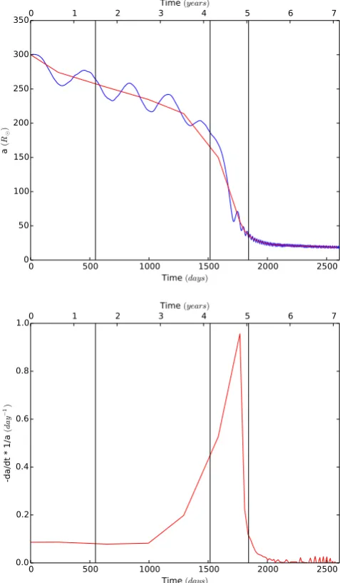
Figure 3. Upper panel: evolution of the separation,a, between the two particles representing the core of the primary and the companion, over the whole simulation time for theENZOsimulation. The blue line represents
the actual separation computed every 0.01 yr. The red line represents the separation averaged over one orbital cycle. The black vertical lines represent, from left to right, the beginning of mass transfer, the beginning of the fast in-spiral phase and the end of the fast in-spiral phase. Lower panel: evolution of the orbital decay, computed on the separation averaged over one orbital cycle for the same simulation.
obtained byP12in their simulations with the companion star slightly
away from the primary surface rather than in contact.
The orbit starts to become elliptical during the rapid in-spiral phase. Using the maxima and minima in the orbital separation evolution after the end of the rapid in-spiral phase, we obtain an
eccentricitye=0.12, in agreement with what was obtained byP12.
The final separation achieved (af) is a crucial output of the CE
simulations.P12identified that CE simulations have final
separa-tions that not only tend to be larger than observed (Zorotovic et al.
2010; De Marco et al.2011), but that depend on the companion/
primary mass ratio (q), a tendency not seen in the observations. By
using the average separation (red line in Fig.3) we estimated the
value of the separation reached at the end of the rapid in-spiral phase
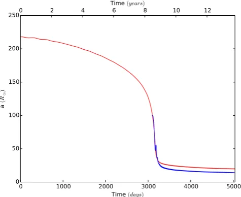
[image:6.595.48.285.59.253.2]Figure 4. Evolution of the separation,a, between the two particles repre-senting the core of the primary and the companion for thePHANTOM simu-lations with initial separations of 100 R(blue curve) and 218 R(red curve). For a clearer comparison of the final separation the blue line has been shifted forward in time by 3096- d, which is the time when the orbital separation of that simulation reaches 100 R.
in ourENZOsimulation to be 36 R, using the criterion described
above and 20 Rif we take the average value at the end of the
sim-ulation (see Table1, where we report the initial conditions and final
outcomes for all past CE simulations including at least a giant). The
separation at the end of the simulation is4 times the smoothing
length, indicating that the end of the in-spiral is not affected by the smoothing length and resolution. Our values of the final separation
are larger than those ofP12, which were 19 and 16 R, for the
criterion defined and final separations, respectively. In other words,
the final separation is larger by 25 per cent for theENZOsimulation
starting with a larger initial separation.
For our firstPHANTOMsimulation, carried out with the same initial
configuration as the simulation ‘SPH2’ ofP12, the final separation
we obtain is 21 Rat 180 d (the end of the dynamical in-spiral
as defined above), 16 Rat 1000 d and 14 Rat the end of the
simulation at 1500 d (blue line in Fig.4). The first two values can
be compared to 21 R at the end of the in-spiral and 18 Rat
1000 d for simulation ‘SPH2’ ofP12. We therefore find a very good
level of agreement in the final separation obtained between the two codes. The small differences are mainly due to the differences in
resolution and the slightly different initial separation of 100 Rthat
we had to adopt because the relaxed star inPHANTOMhas a larger
radius (R=93 R; defined using the volume-equivalent definition
of Nandez et al.2014) compared to the radius of the star stabilized
in simulation ‘SPH2’ ofP12(R=83 R).
The secondPHANTOMsimulation, carried out with an initial
sep-aration of 218 R, reaches a final separation of 29 R, using the
criterion to define the end of the rapid in-spiral described above or
22 Rat the end of the simulation (5050 d). We can compare these
values (29 and 22 R) to those obtained withPHANTOMin an initial
binary configuration similar to that used byP12(21 and 16 R).
The visual comparison is shown in Fig.4, where we plot the
evolu-tion of the separaevolu-tions of our twoPHANTOMsimulations by shifting
the simulation starting at 100 Rby 3096 d to a time when the other
simulation, starting at 218 Rhas a separation of 100 R. The two
PHANTOM simulations show final orbital separations that differ by
38 per cent, corroborating the conclusion drawn from comparing
the twoENZOsimulations that the final orbital separation increases
by including phases before the fast in-spiral.
3.2 Envelope ejection
To determine the extent to which the envelope is unbound we de-termined whether gas has total energy larger than zero. The total energy can be calculated including or excluding thermal energy, where the former prescription results in more unbound gas. Ivanova
& Chaichenets (2011) discussed how it is the enthalpy rather than
the thermal energy that needs to be included when determining whether a gas parcel is bound or not. Using enthalpy instead of thermal energy increases the unbound mass very marginally. In this work, where not otherwise specified, we include thermal energy in the computation of the bound and unbound mass.
For theENZOsimulation we present the density slices in the orbital
and perpendicular planes in Fig.5. In the first and middle columns
we compare the distribution of unbound gas both using thermal energy (left-hand column) and not (middle column), to distinguish between gas acceleration and gas heating. The initial unbinding event (first two rows, left-hand columns) happens because of heating of the gas falling into the potential well of the companion during the mass transfer phase, which is why this unbound material is not
recorded on Fig.5, middle column. This unbound material has very
low mass. Later, during the rapid in-spiral phase (Fig.5, last three
rows, left-hand and middle columns) far more mass is unbound because it is accelerated above the escape velocity as demonstrated by the similarity of the left-hand and central columns.
Similarly to what was reported in previous work (Sandquist et al.
1998, Ricker & Taam2012; Ohlmann et al.2016a), we observe that,
while the pre-contact interactions do not accelerate the envelope gas to supersonic speeds, during the in-spiral a bow shock forms in front of the companion followed by spiral shocks generated both by primary’s core and the companion. This behaviour is showed in
Fig.6, where we plot the envelope Mach number and the gas entropy
in the orbital plane during the rapid in-spiral (lasting from 1515 d, or 4.2 yr, to 1840 d, or 5 yr, from the beginning of the simulation). The spiral shocks wind around the binary and are stronger closer to the point masses, as highlighted by the entropy distribution in
the last two panels of Fig.6(right-hand column). We note that the
high entropy in the peripheral regions in the first two slices of Fig.6
(right-hand column) is due to residual ‘vacuum’ gas with very high temperature.
The evolution of the unbound gas can be followed only inside
the simulation box due to the grid nature ofENZO. However, we
estimated whether the mass that leaves the box is bound or unbound in the following way. We calculated the fraction of unbound gas contained within the box boundary (i.e. within the six, one cell thick, box faces) and we assumed it to be representative of the fraction of unbound gas between code outputs (which take place
every 3.65 d= 0.01 yr). We then multiplied this fraction by the
mass that leaves the box between code outputs.
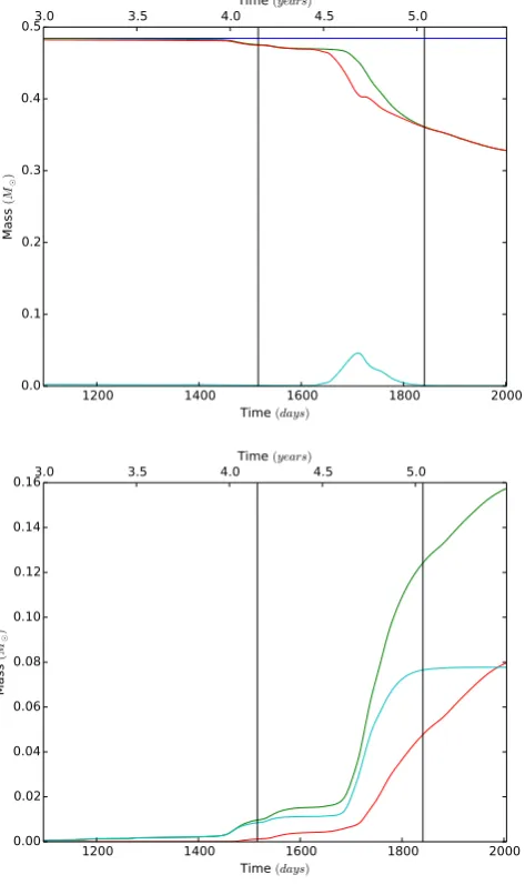
The estimate of the total unbound mass leaving the box is shown
in Fig.7(lower panel). Our approximation is consistent with the
total amount of mass that leaves the box during the simulation,
shown in Fig.7(upper panel). The first unbound mass leaves the
box at approximately 1500 d, at the onset of the rapid in-spiral, but the bulk of the mass flows out during the rapid in-spiral phase (between approximately 1750 and 1900 d). The total mass unbound
in the simulation amounts to 8×10⁻²M
, or 16 per cent of the
initial envelope mass. The unbound mass is 14 per cent, if we do
MNRAS464,4028–4044 (2017)
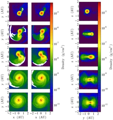
Figure 5. Left-hand panel, left-hand column: density slices perpendicular to thez-axis in the orbital plane after (from top to bottom) 887, 1381, 1653, 1774 and 1840 d from the beginning of theENZOsimulation. The point mass particles representing the core of the primary and the companion are shown as black
dots, while the white regions represent the unbound gas. The size of the black dots is not representative of any property of the point masses and is chosen only to highlight them. Left-hand panel, right-hand column: same as the left-hand column, but excluding thermal energy (Eth) in the computation of the
bound/unbound mass elements. Right-hand panel: density slices perpendicular to the orbital plane atx=0, taken at the same times as the left-hand panels.
not include thermal energy and 17 per cent, if we use the enthalpy
as suggested by Ivanova & Chaichenets (2011). P12found that
10 per cent of the initial envelope mass was unbound, which should be compared to our 16 per cent. This increase likely represents the effect of a larger initial separation.
Most of the ejecta are expected to flow away close to the orbital plane, where the gas is accelerated by the orbiting particles. This
was already borne out by the simulations of Sandquist et al. (1998)
and is clearly seen in Fig.5(right-hand panel). Fig.8demonstrates
how the envelope is ejected around the binary over time. We divide the computational domain into six pyramids centred at the centre of the box and whose bases are the six faces. We plot the mass in
pairs of pyramids aligned with each of the three directions,x,yand
z. Initially the mass is equally distributed in the three pairs of
pyra-mids as the star resides at the centre of the box. Later the mass in the pyramid pairs oscillates as the giant moves along its orbit. The de-crease of the peaks in the green line during the rapid in-spiral phase
in Fig.8marking approximately the completion of a full orbital
revolution, demonstrates a decrease in the mass contained in the
z direction in favour of mass contained in the other two
direc-tions. The decreasing amplitude of the oscillations over time indi-cates that the gas distribution becomes more and more independent of the orbital motion of the two particles, as the interaction pro-ceeds. Towards the end of the CE, as the oscillations cease, more mass is being ejected out of the simulation box highlighting how the rapid in-spiral rapidly lifts the envelope, disrupting the primary star.
For thePHANTOMsimulations, we plot the evolution of the bound
and unbound components of the mass in Fig.9. The first simulation,
starting from an initial orbital separation of 100 R, shows that the
unbinding of the envelope mass begins right after the simulation is started and terminates around 80 d, before the separation has
levelled off (Fig.9, upper panel). The unbinding is almost entirely
caused by gas accelerated above escape velocity, while heating plays a minor role. Both these results are in agreement to what
was obtained byP12’s ‘SPH2’ simulation. The mass unbound is
approximately 13 per cent of the envelope mass, compared to
ap-proximately 10 per cent for ‘SPH2’ ofP12. Again, we think that
these differences are due to differences in the code used and in the slightly larger initial separation.
Figure 6. Left-hand panel: Mach number slices perpendicular to thez-axis in the orbital plane for theENZOsimulations, after (from top to bottom) 887, 1381,
1653, 1774 and 1840 d from the beginning of the simulation. The point mass particles representing the core of the primary and the companion are shown as black dots. The size of the black dots is not representative of any property of the point masses and is chosen only to highlight them. The Mach number equal to unity contours are marked with a blue line. Right-hand panel: same as for the left-hand panel, but for the entropy distribution.
The second PHANTOM simulation starts instead from an initial
orbital separation of 218 R. In this case the unbinding of the mass
begins gradually while the companion approaches the primary star, but before the onset of the rapid in-spiral. Then as soon as the rapid in-spiral is triggered the bulk of the mass is ejected and unbound
(Fig.9, lower panel). This behaviour is very similar to what we
obtained for ourENZOsimulation starting from an initial separation
of 300 R. The mass unbound in the simulation is 16 per cent of the
envelope mass, marginally larger than the 13 per cent for the same simulation starting with a lower initial separation. The increased amount of mass unbound is therefore in line with what we obtained
for ourENZO simulations. Similarly to what was observed in the
ENZOsimulation, and in line with previous work, the envelope is
mainly expelled in the orbital plane and a series of spiral shocks are produced while primary core and companion in-spiral towards each other.
3.3 Tidal bulges
As explained in Section 2.2, the pre-contact phase in our simulation takes place over much shorter time-scales than it would in nature. The short pre-contact time-scale observed in our simulation is due to deformations created on the primary by the insertion of the com-panion into the computational domain. This is likely the result of the lack of stabilization of the binary in the corotating frame, discussed in Section 2.2.
MNRAS464,4028–4044 (2017)
Figure 7. Upper panel: evolution of the gas mass inside theENZOsimulation domain over time. The blue line represents the value of the initial gas mass contained in the domain and is plotted for comparison, while the green line shows the evolution of the total mass contained inside the box. The red and cyan lines show, respectively, the bound and unbound components of the mass. Lower panel: cumulative mass of the gas flowing out of the simulation box over time for the same simulation. Line colours have the same meaning as for the upper panel. The black vertical lines in both panels correspond to the beginning and end of the rapid in-spiral and both plots are limited to the part of the simulation where significant mass is lost from the box.
A simple order of magnitude analytical estimate of the mass,
δM1, contained in the tidal bulges of the primary, for equilibrium
tides, can be obtained from Zahn (2008):
δM1≤M2
R1
a 3
, (1)
whereM1,M2,R1andaare the masses of the primary, secondary,
the radius of the primary and the orbital separation, respectively.
For the purpose of this calculation we only varyawith time, while
leavingR1constant, hence the value ofδM1oscillates due to the
eccentricity that develops (Fig.3, upper panel).
In Fig.10we compare this analytical estimate with the bound
mass residing outside the initial equilibrium radius of the primary
[image:10.595.49.286.61.460.2]forENZO(solid line) andPHANTOM(dashed line). The insertion of the
Figure 8. Gas mass inside the simulation domain versus time for the gas located in six pyramids whose bases are the six faces and whose vertexes are at the centre of the domain, for theENZOsimulation. The two pyramids along thex-axis are in blue, along they-axis are in red and along thez-axis are in green. The cyan line shows the sum of thexandycontributions to highlight the behaviour of the mass ejection in the orbital plane. The black vertical lines show the estimated beginning of the Roche lobe overflow phase and the beginning and end of the rapid in-spiral phase.
companion into the simulations’ domain triggers some oscillations
on a time-scale of the order of the dynamical time of the star (21 d).
Over the pre-contact phase there is also a gradual expansion of the star, seen as an increasing trend of the mass outside its original volume. The oscillation is caused by the mass distribution acquiring two small opposite bulges that are initially aligned with the direction
of the companion, but which then disappear and reappear at 90◦to
the original direction. This generates the relatively strong torques that contribute to the fast decrease of the orbital separation during the pre-contact phase.
Both simulations show that the bulge mass is commensurate with
the analytical approximation. The oscillation is smaller inPHANTOM
due to the fact that SPH is more stable to surface deformations
compared to the grid-based ENZO. This may be the reason why
the tidal in-spiral is slower inPHANTOMthanENZO. Another reason,
discussed more in depth in Section 3.5, could be thatENZOconserves
angular momentum less well thanPHANTOM.
At 1515 d in theENZOsimulation, gravitational drag between the
companion and the surrounding gas becomes the main mechanism exchanging energy and causing the decrease of the orbital separation
(see Ricker & Taam2012and discussion below in Section 3.4). This
regime change is evident in Fig.3, at the location of the vertical line
representing our estimation for the beginning of the rapid in-spiral.
3.4 Evolution of the gas velocities and density in proximity to the companion
The mechanism behind the energy and angular momentum ex-change that drives the in-spiral is gravitational drag (Ricker & Taam
2012). Gravitational drag is caused by the gas that flows past the
moving body (in our case the companion star), forming a wake with higher density behind it that gravitationally pulls on it, slowing the body down. The gravitational drag experienced by a body im-mersed in a fluid depends on the body’s mass, the fluid density, the velocity contrast between the body and the fluid and on the Mach
Figure 9. Upper panel: evolution of the gas mass for thePHANTOM
sim-ulation starting with an initial separation of 100 R. The green line shows the evolution of the total mass. The red and cyan lines show, re-spectively, the bound and unbound components of the mass. Lower panel: evolution of the gas mass for thePHANTOMsimulation starting with an initial separation of 218 R. Colours are the same as those of the upper panel.
number of the body. Approximations for the gravitational drag are
given by Iben & Livio (1993,Fdrag∝(M2ρvrel2)/(v2rel+c2s)2, for the
subsonic motion regime) and by Ostriker (1999) who calculated a
more detailed formula, carefully considering the effects of the Mach number.
It is fundamental to determine whether simulations accurately reproduce the effects of gravitational drag because this determines in turn when the companion in-spiral terminates and, as a result, the amount of orbital energy deposited. Is the end of the in-spiral due to the decreasing density around the particles, the corotation of the surrounding gas or a change in the Mach regime (as was the
case in the simulations of Staff et al.2016b)? Does the density
gra-dient affect the force as questioned by MacLeod & Ramirez-Ruiz
(2015)? How does the interplay of resolution and smoothing length
affect the simulation (Staff et al.2016a)? It is well known that the
particles will not approach closer than approximately two smooth-ing lengths, effectively because their potentials are flat within that
Figure 10. Mass in the tidal bulges of the primary star overtime during the pre-contact phase, estimated from theENZOsimulation data (solid blue line), from thePHANTOMsimulation with an initial separation of 218 R data (dashed blue line) and from the analytical formula (dotted red line).
distance. However, less clear are the effects that not resolving a
radius of the order of the Bondi radius (Bondi1952) around the
particles will have on the drag force (Staff et al.2016b).
In Fig. 11we display the evolution of the density profile
be-tween the two cores for theENZOsimulation, showing only the part
between the particles (upper panel), or the entire computational do-main (lower panel). The density profile changes smoothly at the beginning of the simulation, with the primary expanding, but it then transitions into a phase of more rapid change at the onset of the rapid in-spiral phase, when the profile flattens and then becomes U-shaped, showing peaks at the locations of both primary’s core
and the companion with densities of 2.8×10⁻⁶ g cm−3for the
primary and 4.6×10⁻⁶g cm−3for the companion. The underlying
density is of the order of 10−6g cm−3at 365–730 d after the start of
the simulation. These values are comparable to those ofP12(their
fig. 13, middle panel).
The gas density in the proximity of the particles at the end of the simulation is high, and is unlikely to be the cause of the observed
slowing down of the in-spiral. From the density profiles Fig.11
(lower panel) it is clear that during the evolution of the system some of the envelope accumulates around the companion. The accumu-lation of mass is negligible until the beginning of the rapid in-spiral phase, during which it starts to increase because the companion is plunging into the denser parts of the envelope. The companion local
density is a factor of a few larger than the density 10–20 Raway
from it. The density gradient underlying the density peak near the companion is small and likely unimportant to the in-spiral.
In Fig. 12 (upper panel) we plot the companion’s speed, the
average local gas velocity projected in the direction of motion of the companion and the average local gas velocity projected in the
direction perpendicular to the motion of the companion for theENZO
simulation. In Fig.12(lower panel) we plot the companion’s Mach
number and the normalized average density near the companion. To calculate the parallel and perpendicular ambient gas velocities we averaged the respective projections for all cells within a volume
with radius 10 R from the companion. The local density was
calculated by averaging the density inside the same volume and the
MNRAS464,4028–4044 (2017)
[image:11.595.308.545.60.251.2]Figure 11. Upper panel: density profile between the core of the primary (located at zero in the abscissa) and the companion (each black dot represents the density at the location of the companion) for theENZOsimulation. Profiles are taken, for clarity, every 110 dumps of the code. Colours represent times as follows: red=0 d, blue=398 d, cyan=796 d, yellow=1194 d, black= 1591 d, orange=1989 d. Lower panel: same as the top panel, but extended to the whole box. The primary’s core is represented by a large black dot while the companion is marked as a smaller dot.
Mach number by averaging the gas sound speed within the same volume.
As was the case for the simulation ofP12, the entire journey of
the companion is subsonic, reaching at most a Mach number of
0.47. This is different from the simulations of Staff et al. (2016b),
where the initial part of the in-spiral was supersonic and the end of the in-spiral phase appeared to coincide with the transition between supersonic and subsonic regimes. No such transition occurs here.
A regime change does however take place at the approximate time of the end of the in-spiral. This change seems to be initiated by the gas near the companion being brought into near corotation at approximately 1750 d. At this point, while the orbital separation is still reducing, there is still a considerable outflow (cyan line in
Fig.12), which eventually leads to a decrease of the local density
after approximately 1870 d (dashed line in Fig.12). At that point the
companion’s velocity’s increase slows down (blue line in Fig.12,
upper panel) as do both components of the local gas velocity (cyan
and green lines in Fig.12, upper panel). By approximately 2100 d,
[image:12.595.46.284.58.423.2]the density has reduced so much (green line in Fig.12, lower panel)
Figure 12. Upper panel: companion velocity (thicker blue line), local av-erage gas velocity projected on the direction of the companion velocity (vgas,, thick green line) and local average gas velocity perpendicular to the direction of the companion velocity (vgas,⊥, thin cyan line) for the ENZOsimulation. The three lines are smoothed with a Savitzky–Golay filter, using 31 coefficients and seventh-order polynomials. Lower panel: compan-ion Mach number (thick blue line) and normalized average gas density in the companion’s proximity (ρ/ρmax, whereρmax1.15×10−5g cm−3;
thin green line). All plots start at the onset of the rapid in-spiral, the vertical solid lines represent the estimated end of the rapid in-spiral and the dashed ones mark the point of maximum density.
that the gravitational drag is very small and the parameters of the binary change very slowly. Most of the unbinding happens at 1700 d,
right after most of the orbital decay has taken place (Fig.3, upper
panel).
To confirm that this trend is not a result of the size of the sphere used to estimate our quantities, we carried out the same test with
spheres of 5 and 20 R. Both show results similar to Fig.12with
the only exception that the gas velocity parallel to the companion direction of motion is overall larger and close to the companion’s velocity for the smaller sphere, as expected. We also note that at the beginning of the in-spiral the local gas has a rotation velocity of
10–20 km s−1, which is a range of values expected for giants spun up by companions.
3.5 Angular momentum and energy conservation
Energy and angular momentum were conserved by the SPH
sim-ulations of P12 at the 1 per cent level. They did not check the
conservation level of their equivalentENZOsimulations, because of
the grid nature of the code which leads to loss of mass off the
simulation box and because their ENZOsimulations showed
simi-lar results to the SPH ones, which suggested a reasonable level of energy conservation.
As mentioned in Section 2, Staff et al. (2016a) quantified the
level of energy non-conservation in grid-based simulations using
ENZOand determined that conservation is improved by selecting a
larger smoothing length of 3 cells rather than what was used byP12
(1.5 cells). The highest resolution in our AMR simulation is the
same as the resolution in the unigrid simulations ofP12. However,
we have adopted the larger smoothing length of 3 cells, which must have weakened the gravitational interaction somewhat compared to
the simulations ofP12.
In the upper panels of Figs13and14we plot various components
of the angular momentum and energy, respectively, in the ENZO
computational domain as a function of time. The behaviour of some of the components is driven by mass-loss out of the computational
domain, which starts at∼260 d (some of the low-density ambient
medium outflows before, but has negligible mass), but is particularly
heavy during the rapid in-spiral phase. In Fig.13we show only thez
component of the angular momentum, that, as expected, dominates over the other components. Additionally, we see that most of the angular momentum resides in the point masses, with an initial value
of∼3.5×1052g cm2s−1. Before 260 d from the beginning of the
simulation, only negligible mass and angular momentum are leaving
the simulation box. The particles’zangular momentum decreases
during the in-spiral. Some of that is transferred to the gas. 5 per cent of the angular momentum is lost due to non-conservation, between the beginning of the simulation and 260 d, while 10 per cent is lost over the first 3 yr, a time at which substantial amount of mass starts leaving the domain. This value is larger (as expected) than for the
SPH simulation ofP12and similar to the 8 per cent of Sandquist
et al. (1998), who estimated it over1000 d of their simulation.
Estimating the level of conservation of energy is even more diffi-cult than the angular momentum, because the low-density medium filling the volume outside the star has a very high thermal energy, even if its total mass is negligible. Even before envelope mass starts flowing out of the computational domain at 260 d, a small amount of this high-energy gas flows out of the box taking with it an energy
of1.3×1045erg (or11 per cent of the initial total energy). This
behaviour is clear in Fig.14: the total energy at the beginning of
the simulation is dominated by the thermal energy of the ‘vacuum’ and by the potential energy between the point mass particles and the gas, with the former continuously decreasing as some of the low-density medium outflows the box; this decrease is mimicked by the total energy at times greater than 260 d. Before this threshold is passed the code conserves energy to the 4 per cent level, similar
to the result of Sandquist et al. (1998).
In Figs13and14, lower panels, we present the angular
momen-tum and energy conservation properties for ourPHANTOMsimulation
with an initial orbital separation of 218 R(similar results were
obtained for the smaller, 100 R, initial orbital separation
[image:13.595.307.543.60.461.2]simula-tion). The angular momentum is conserved to the 0.03 per cent level
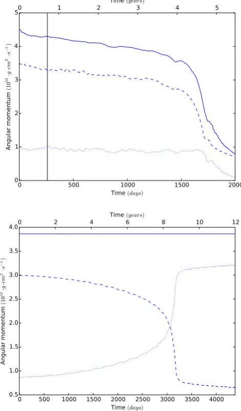
Figure 13. Upper panel: evolution of thezcomponent of the angular mo-mentum with respect to the centre of mass of the system for gas (dotted line), particles (dashed line) and their sum (solid line), inside theENZOsimulation domain. The black vertical line represents the moment when the envelope mass starts leaving the box (260 d). Lower panel: evolution of thez com-ponents of the angular momentum for thePHANTOMsimulation starting at 218 R. The line styles are the same as for the upper panel.
over the entire simulation time, better than what obtained byP12
withSNSPH(Fig.13, lower panel). Additionally, mass conservation in SPH simulations allows us to highlight the transfer of angular
momentum from the orbit (dashed line in Fig.13, lower panel) to
the envelope gas (dotted line in Fig.13, lower panel).
Total energy (thick black line in Fig.14, lower panel) is conserved
inPHANTOMat the 0.1 per cent level, again better than what obtained byP12withSNSPH. By comparing upper and lower panels of Fig.14, one can also notice the magnitude of the contribution of the hot
‘vacuum’ to theENZOenergy budget.
Both ENZO (initial separation 300 R) and PHANTOM (initial
separation 218 R) simulations reach the onset of the rapid
in-spiral over similar, non-realistic time-scales of the order of years
(Section 3.3). SincePHANTOMconserves angular momentum well,
we deduce that non-conservation inENZO is not the main factor
MNRAS464,4028–4044 (2017)
Figure 14. Upper panel: components of the energy as a function of simu-lation time in theENZOdomain: total energy (thick black line), total kinetic energy (solid black line), total potential energy (dashed black line), total (= gas) thermal energy (dotted black line), gas kinetic energy (solid red line), gas potential energy (dashed red line), point mass kinetic (solid yellow line), point mass to point mass potential (dashed yellow line) and point mass to gas potential (dashed cyan line). The black vertical line represents the mo-ment when the envelope mass starts leaving the box (260 d). Lower panel: conservation of the components of the energy for thePHANTOMsimulation starting at 218 R. The colours are the same as for the upper panel. driving the orbital shrinkage, though we cannot exclude that it plays a role.
4 C O M PA R I S O N W I T H P U B L I S H E D S I M U L AT I O N S
Here we carry out a comparison of CE simulations containing at
least one giant (Rasio & Livio1996; Sandquist et al.1998,2000;
Passy et al.2012; Ricker & Taam2012; Nandez et al.2015; Nandez
& Ivanova2016; Ohlmann et al.2016a), highlighting possible trends
or aspects that need further clarification. We do not include those
simulations carried out by Staff et al. (2016a) that started with
highly eccentric orbits. All the final results of these simulations
are summarized in Table1and we display results in Fig.15. All
the simulations, except that of Nandez et al. (2015) are carried out
with codes that include similar physics and can be more directly compared.
4.1 Side-by-side code comparison
The only side-by-side code comparison that can be carried out is
amongENZO,SNSPHandPHANTOMfor which almost identical
simu-lations were carried out. The comparison between the first two was
already carried out byP12. Here we only add thatSNSPHresults in
final separations that are approximately 10 per cent larger than for
ENZO. The relative difference does however increase for simulations
with very low mass companions (0.1 M).
The comparison betweenSNSPH(simulation SPH2 inP12) and our
ownPHANTOMsimulation shows that, at the criterion point, the final separations are the same within one solar radius, while at 1000 d the PHANTOMseparations is 10 per cent smaller, but has the same value as
theENZOsimulation. We conclude that code-to-code differences for
these three codes and for this parameter space are within 10 per cent
for simulations with companions more massive than∼0.3 M.
4.2 The final orbital separation as a function ofM2/M1
Comparing the fiveENZOsimulations ofP12with each other, or their
fiveSNSPHsimulations with each other or, to an extent, comparing
two of the simulations of Sandquist et al. (1998) for which only
M2 was changed, we conclude that the final separation increases
for increasing value ofM2, for the same value ofM1. It is
diffi-cult to compare with the other simulations, because although two
simulations may have the same value ofq, the binding energies of
the primaries’ envelope could be vastly different (but see Section
4.3). Some of the simulations of Nandez & Ivanova (2016) carried
out with the same primary and different secondary masses could be used to carry out this kind of analysis were it not for the very narrow range of mass ratios available which lead to effectively the same final separation.
Sandquist et al. (1998) also compared two simulations with
dif-ferent primaries and the sameq. The simulation with the more
ex-tended, lower binding envelope energy primary has a much larger
final separation (see Table1), but we did not plot it because the
final separation cannot decrease much below the resolution times the particles’ smoothing length and in that simulation the two values are almost the same.
The post-CE binary observations of Zorotovic et al. (2011) show
that post-CE binaries with post-RGB primaries (identified by a
mass smaller than 0.5 M) have systematically smaller separations
than post-CE binaries with post-asymptotic giant branch (AGB)
pri-maries (which have masses larger than 0.5 M). They also show a
marginal correlation, though statistically ‘real’, between secondary mass and post-CE orbital separation. The latter conclusion is in line with the simulations, though clearly the signal in the data is diluted by the range in primary masses for each secondary mass (see below).
4.3 The final orbital separation as a function of primary mass or envelope binding energy
The simulations of Rasio & Livio (1996), Nandez et al. (2015),
Nandez & Ivanova (2016), Ohlmann et al. (2016a) and some of
the simulations of Sandquist et al. (2000) produce distinctly lower
separations, at a given mass ratio, even accounting for their
differ-ent values ofM2. We ascribe this difference to heavier and/or more