Exploiting historical registers: Automatic methods for coding c19th and c20th cause of death descriptions to standard classifications

Exploiting historical registers: Automatic methods for

coding c19th and c20th cause of death descriptions to

standard classifications

Jamie Carson

, Graham Kirby

, Alan Dearle

, Lee Williamson

,

Eilidh Garrett

, Alice Reid

, Chris Dibben

1

School of Computer Science, University of St Andrews e-mail: {jkc25, graham.kirby, alan.dearle}@st-andrews.ac.uk 2_{Longitudinal Studies Centre Scotland, University of St Andrews}

e-mail: {lepw, cjld}@st-andrews.ac.uk

3_{Department of Geography, University of Cambridge} e-mail: [email protected], [email protected]

Abstract

The increasing availability of digitised registration records presents a significant oppor-tunity for research. Returning to the original records allows researchers to classify de-scriptions, such as cause of death, to modern medical understandings of illness and dis-ease, rather than relying on contemporary registrars’ classifications. Linkage of an indi-vidual’s records together also allows the production of sparse life-course micro-datasets. The further linkage of these into family units then presents the possibility of reconstruct-ing family structures and producreconstruct-ing multi-generational studies. We describe work to de-velop a method for automatically coding to standard classifications the causes of death from 8.3 million Scottish death certificates. We have evaluated a range of approaches us-ing text processus-ing and supervised machine learnus-ing, obtainus-ing accuracy from 72%-96% on several test sets. We present results and speculate on further development that may be needed for classification of the full data set.

Keywords: machine learning, linkage

Acknowledgements: This work is supported by the Wellcome Trust and the Scottish Health Informatics Programme.

1.

Introduction

classify descriptions, such as cause of death, to modern medical understandings of illness and disease, rather than relying on contemporary registrars’ classifications. Linkage of an individual’s records together also allows the production of sparse life-course micro-datasets. The further linkage of these life-course micro-datasets into family units then presents the possibility of reconstructing family structures and producing multi-generational studies. This type of data therefore presents the possibility of researching important characteristics of both the historic and the modern population, particularly the inheritance of various traits and vulnerabilities.

There are of course significant methodological issues to overcome before this type of data can be exploited in the way outlined. This paper describes work being carried out in Scot-land, to develop a method for automatically processing the 8.3 million causes of death recorded on death certificates from 1855 to the present day. These are being made ready for analysis by the ‘Digitising Scotland’ project (Dibben, Williamson and Huang, 2012), funded by the UK’s Economic and Social Research Council. This project is jointly run by the University of St Andrews and National Records of Scotland (Scotland’s national sta-tistical agency).

There are two key problems: firstly, how to consistently code cause of death over the en-tire 150 year period so that researchers can explore changing patterns and trends; and secondly, how to automate this process so that the majority of records do not need to be manually coded. In this paper we focus on the second of these problems: developing methods to automatically classify narrative cause of death descriptions into a fixed set of standard classifications.

2.

Data Sets

The target data set is, as described, the complete set of all 8.3 million causes of death rec-orded in Scotland from 1855 to present day. They need to be coded to the ICD-10 classi-fication (World Health Organization, 1990). Transcription of these records will com-mence in early 2013, so we do not currently have this data in electronic form.

For our experiments in automatic classification we used a number of smaller data sets, all from the latter half of the C19th, for which we already had cause of death codings pro-duced by expert historians. The cause of death string in some records contains a single cause of death, while in others it includes both primary and contributory factors. In the majority of such cases the factor listed first would now be considered the primary factor, but this is not universally true. All of the data sets were completely anonymised before any processing in our classification experiments.

Tasmania: 93,000 records (22,000 unique) from Tasmania in the period 1838-1899 (Gunn and Kippen, 2008). For this data set we have only the set of unique causes; we do not know the number of occurrences of each one. These records are coded into 36 distinct classes.

Massachusetts: 47,000 records (13,000 unique) from Massachusetts in the period 1850-1912, provided by Susan Leonard. See (Leonard, Anderton and Swedlund, 2012) for more information on the project and access to tidied forms of the data. These records are coded into 170 distinct classes.

3.

Classification Methods

We have evaluated several methods for automating coding. For each of the methods we contrast our automatic coding against the assumed ‘gold standard’ of the historian coding. We explored three approaches:

• parsing using regular expressions • natural language processing • machine learning

3.1 Parsing

Experiment 1. The idea of this approach is to design, after studying examples of input strings and the corresponding actual codings, a simple parser that can extract substrings equivalent to the desired coding. Using a regular expression processor, we implemented a sequence of transformations, including:

• discarding multiple causes of death where indicated by numbering • discarding parenthesised phrases

• discarding linking phrases such as ‘and’, ‘from’, ‘due to’, ‘owing to’, etc • discarding references to duration of illness

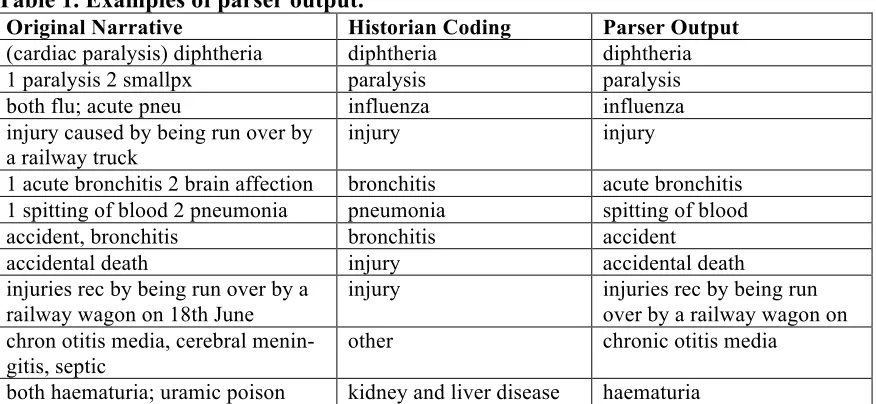
Table 1. Examples of parser output.

Original Narrative Historian Coding Parser Output

(cardiac paralysis) diphtheria diphtheria diphtheria

1 paralysis 2 smallpx paralysis paralysis

both flu; acute pneu influenza influenza

injury caused by being run over by a railway truck

injury injury

1 acute bronchitis 2 brain affection bronchitis acute bronchitis

1 spitting of blood 2 pneumonia pneumonia spitting of blood

accident, bronchitis bronchitis accident

accidental death injury accidental death

injuries rec by being run over by a railway wagon on 18th June

injury injuries rec by being run

over by a railway wagon on chron otitis media, cerebral

menin-gitis, septic

other chronic otitis media

both haematuria; uramic poison kidney and liver disease haematuria

It can be seen that 4 of the 11 examples were classified correctly by the parser. This is not, however, a representative sample of the data set; these examples have been chosen to illustrate the effects of the various transformations.

The example in the last row illustrates a fundamental limitation of this approach. It is in-capable of producing a classification that contains phrases not appearing in the original— unless produced by a ‘hard-wired’ shorthand expansion such as that of ‘flu’ in the third row. A related issue is that the classifier has no ‘knowledge’ of the set of desired classifi-cations, and so makes no attempt to map to the best candidate from that set.

A further methodological limitation is that the approach relies on being able to identify sufficient commonality in the phrasing of the cause of death narratives to be able to de-sign appropriate parsers; this involves a de-significant degree of manual analysis of the source text, and the resulting parsers may not give good results on other data sets.

3.2 Natural Language Processing

We investigated the potential for more sophisticated grammatical analysis, and consid-ered using the OpenNLP toolkit (Apache Software Foundation, 2010) to produce parse trees representing the grammatical structure of the cause of death strings. However, we were unable to find a straightforward method for mapping such parse trees to the desired standard coding. Knowing the grammatical structure was not helpful in identifying any link to the standardised coding, since these are essentially ‘term-driven’ with little varia-tion in grammar.

3.3 Machine Learning

mini-mising error. The function f can then be used to assign an output class to previously un-seen data.

Experiment 2. The Mahout machine learning framework (Apache Software Foundation, 2011) was used to perform classification using three separate learning algorithms:

• Stochastic Gradient Descent (SGD) (Zhang, 2004) • Naive Bayes (Langley, Iba and Thompson, 1992)

• Complementary Naive Bayes (Rennie, Shih, Teevan and Karger, 2003)

We separately tested a subset of the Kilmarnock data comprising unique records only. It was expected that classification accuracy would be lower on this than on the full data set, since the benefit of reinforcement by redundant data in the training set would be lost. The purpose was to obtain some indication of the magnitude of this accuracy reduction, since in some circumstances only the unique records may be available—as is the case for the Tasmania data in this work.

Experiment 3. We experimented with combining the parser with a machine learning classifier, in the hope that some simple cleaning of the input data to the classifier would improve its performance. We used the parser to transform the original cause of death de-scriptions before feeding the results to the SGD classifier. The results were better than stand-alone SGD on some data sets, and worse on others.

Experiment 4. When we compared the individual per-record classification decisions of the two-phase classifier described above with those made by the stand-alone SGD classi-fier, we noticed that the pre-processing had a negative effect in some cases. Since the SGD implementation provides a numerical measure of confidence for each classification decision, we then used this measure to decide between the classifier with pre-parsing and the stand-alone version, on a per-record basis. We trained both versions, used both to classify each test record independently, and then picked the decision with the higher con-fidence value attached. This gave the best results so far.

Experiment 5. Our next step was to try an ensemble method (Dietterich, 2000) combin-ing the decisions of multiple machine learncombin-ing classifiers. We ran each of the three classi-fiers, plus SGD with pre-processing, and the compound classifier from experiment 4, and for each record picked the most popular classification from the resulting five decisions.

Experiment 6. We now wanted to use confidence measures to decide between machine learning classifiers, in a similar style to experiment 4. We used an ensemble containing the three core classifiers, plus SGD with pre-processing. The two Bayesian classifiers do not, however, generate confidence measures. To address this, we examined the classifica-tion decisions and confidence levels produced by the SGD classifier in previous experi-ments, and identified a static confidence threshold value that corresponded approximately to a 50% probability of being correct.

ex-ceeded the threshold the corresponding decision was selected. Otherwise the decision of one of the Bayesian classifiers was chosen at random.

Experiment 7. In the final ensemble variation, we generated proxy confidence values for the Bayesian classifiers, and then selected the classifier with the highest confidence. Be-fore the classification tests we ran the Bayesian classifiers over the training set. For each class X we recorded the proportion of records classified as X that should in fact have been so classified. We could then treat this value as a crude approximation of the probability that a classification decision of X would be correct, or after suitable mapping to a differ-ent scale, a proxy confidence measure.

4.

Results

In the following discussion we abbreviate the names of the data sets as: KM-F for the full Kilmarnock set; KM-U for the unique Kilmarnock records; TAS-U for the unique Tas-mania set; and MASS-F for the full Massachusetts set.

Experiment 1. The parsing classifier developed for the Kilmarnock data was evaluated on that data set. Since this classifier did not require training, the entire data set was used for testing, and only a single testing run was required. The accuracy obtained was 44%, relative to the expert-coded classifications—rather low as expected for reasons previously discussed.

Experiment 2. Table 3 shows the range of accuracies obtained using the various classifi-ers, with the number of test runs shown in brackets. For each run on each data set, 80% of the records were randomly selected as the training set, and the remainder used for testing.

Table 3. Classification accuracy of machine learning classifiers.

KM-U (5) KM-F (5) TAS-U (4) MASS-F (2)

SGD 22-68% 92-93% 74-85% 19-27%

Naive Bayes 65-67% 89-90% 77-77% 82-82%

Complementary Naive Bayes 65-67% 89-90% 77-77% 82-82%

As expected, classification performance was generally poorer on the unique record data sets, leading us to speculate that performance on the Tasmania data might be improved if the duplicate records were known. The SGD classifier exhibited much greater variation in accuracy between runs than the two Bayesian classifiers, which also appeared to perform identically.

Table 4. Classification accuracy of SGD classifier on unique Kilmarnock records us-ing various proportions for trainus-ing, and testus-ing on remainder.

10% 20% 30% 40% 50% 60% 70% 80% 90%

SGD

48-51%

56-58%

59-61%

60-64%

64-66%

63-67%

62-67%

65-68%

66-68%

It appears from these results that for the Kilmarnock data set the bulk of the training ben-efit can be achieved with 20% of the records; further increases in the training set size yield only small improvements. This is encouraging with respect to the eventual goal— classification of millions of initially un-coded records—for which the relevant question is ‘how small can the training set be while retaining acceptable accuracy?’ We will need to be able to estimate this in order to decide how many records need to be (expensively) hand-coded at the outset of the main classification activity.

Experiment 3. Table 5 shows the effect of combining the SGD classifier with version 1 of the parser classifier. First, the parser was applied to all records in the data set, with each result replacing the original cause of death string. The SGD classifier was then used to classify the modified strings, using an 80/20 training/testing split as before, over 4 runs.

Table 5. Classification accuracy of SGD classifier operating on output from parser.

KM-U (5) KM-F (5) TAS-U (4) MASS-F (2)

SGD with pre-parsing 25-78% 88-93% 65-72% 20-28%

Experiment 4. Table 6 shows the results of using the confidence measure output by the SGD implementation to decide, on a per-record basis, between the alternative classifica-tions.

Table 6. Classification accuracy of SGD with confidence-decided pre-processing.

KM-U KM-F (5) TAS-U (4) MASS-F (2)

SGD with confidence-decided pre-processing

26-81% 92-96% 79-88% 20-28%

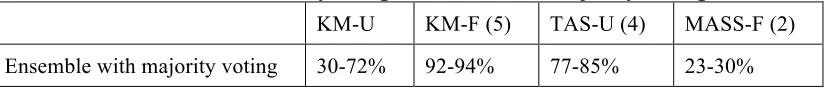
Experiment 5. Table 7 shows the results for the ensemble classifier using 5 pre-processor/classifier combinations, determining the overall classification for each record by majority voting.

Table 7. Classification accuracy using ensemble with majority voting.

KM-U KM-F (5) TAS-U (4) MASS-F (2)

Experiment 6. Table 8 shows the results for the ensemble classifier using confidence measures, where available, to choose between individual classifiers.

Table 8. Classification accuracy using ensemble with confidence-decided selection.

KM-U KM-F (5) TAS-U (4) MASS-F (2)

Ensemble with confidence-decided selection

72-84% 95-96% 87-93% 84-84%

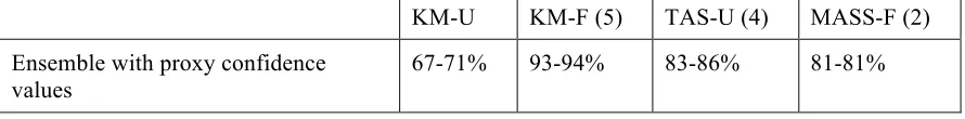
Experiment 7. Table 9 shows the results of the ensemble classifier using confidence measures to select between classifiers, with proxy values generated for the Bayesian clas-sifiers.

Table 9. Classification accuracy using ensemble with proxy confidence values.

KM-U KM-F (5) TAS-U (4) MASS-F (2)

Ensemble with proxy confidence values

67-71% 93-94% 83-86% 81-81%

5.

Conclusions

Table 10 summarises the performance of the best classifier for each of the data sets. The right-most column shows the ratio of records to classes for each data set.

Table 10. Summary of best classifiers for various data sets.

Data set Accuracy Best classifier Records/class

KM-U 72-84% Ensemble with confidence-decided selection 71

KM-F 95-96% Ensemble with confidence-decided selection 252

TAS-U 87-93% Ensemble with confidence-decided selection 611

MASS-F 84-84% Ensemble with confidence-decided selection 276

As expected, the accuracy achieved for the unique Kilmarnock records was significantly worse than that for the full data set. This may be due to the beneficial redundancy in the full data set, in terms of training effect, or simply due to the training set being larger for the full data set, since the same training/testing ratio was used in all cases. If the latter factor is significant, then it might have been a fairer comparison to have fixed the training set size for all data sets rather than the ratio. However, the results shown in Table 4 sug-gest that performance is not particularly strongly affected by training set size.

The ensemble with confidence-decided selection (experiment 6) gave the best perfor-mance for all data sets, taking both accuracy and consistency into account. Therefore this appears to be the most promising approach.

Looking ahead to the task of classifying the full Scottish data set, we will conduct a simi-lar exercise on a sample of the records as they become available, in order to decide which classification approach should be employed. Even before this, we plan several follow-up experiments to those already performed:

• We will perform a manual analysis of the incorrectly classified records, looking for any common patterns that might be candidates for special cases being added to the pre-processor.

• We will investigate whether the classifiers could be applied, in a later phase, to the problem of identifying records likely to have been incorrectly classified—in which case a secondary classification process could be performed to prioritise cer-tain records for manual checking.

• We will repeat the main experiments on a data set containing 200,000 modern death records that are already coded to ICD-10. We expect that classification ac-curacy may be better for these, since we expect modern narrative descriptions to be more tightly focused and to exhibit less variation.

• Using the same data set we will investigate the effect of varying the granularity of classification, for example coding to sub-categories of ICD-10.

• We will investigate the applicability of this work to the classification of occupa-tions and family names (the problem in the latter case being to code to standard spellings).

Regarding the methodology for performing classification of a given large-scale data set, we will investigate the scope for automating:

• the selection of the most suitable classifier (whether stand-alone or ensemble), guided by experiments on samples from the data set;

• the determination of the minimum size training set then required to be hand-coded, to achieve a given acceptable level of accuracy.

References

Apache Software Foundation. (2010). Apache OpenNLP. Available at: http://opennlp.apache.org/ (Accessed January 29, 2013).

Apache Software Foundation. (2011). Apache Mahout: Scalable Machine Learning and Data Mining. Available at: http://mahout.apache.org/ (Accessed January 29, 2013). Dibben, C. J., Williamson, L. E. and Huang, Z. (2012). Digitising Scotland. Economic

and Social Research Council, ES/K00574X/1.

Dietterich, T. G. (2000). Ensemble Methods in Machine Learning. In Multiple Classifier Systems. Berlin, Heidelberg: Springer (Vol. 1857, pp. 1–15).

Gunn, P. and Kippen, R. (2008). Household and Family Formation in Nineteenth-Century Tasmania, Dataset of 195 Thousand Births, 93 Thousand Deaths and 51 Thousand Marriages Registered in Tasmania, 1838-1899. Australian Data Archive. Australian National University, Canberra.

Langley, P., Iba, W. and Thompson, K. (1992). An Analysis of Bayesian Classifiers. 10th National Conference on Artificial Intelligence, AAAI Press, 223–228.

Leonard, S. H., Anderton, D. L. and Swedlund, A. C. (2012). Grammars of Death. Uni-versity of Michigan/ICPSR. Available at:

https://sites.google.com/a/umich.edu/grammars-of-death/home (Accessed January 29, 2013).

Mitchell, T. M. (1997). Machine Learning. McGraw-Hill, Inc.

Reid, A., Davies, R. and Garrett, E. (2002). Nineteenth-Century Scottish Demography From Linked Censuses and Civil Registers: a ‘Sets of Related Individuals’ Approach. International Journal of Humanities and Arts Computing, 14(1-2), 61–86.

Reid, A., Garrett, E., Davies, R. and Blaikie, A. (2006). Scottish Census Enumerators’ Books: Skye, Kilmarnock, Rothiemay and Torthorwald, 1861-1901. Economic and Social Data Service. Available at: http://www.esds.ac.uk/

findingData/snDescription.asp?sn=5596 (Accessed January 30, 2013).

Rennie, J. D. M., Shih, L., Teevan, J. and Karger, D. R. (2003). Tackling the Poor As-sumptions of Naive Bayes Text Classifiers. 20th International Conference on Ma-chine Learning. Retrieved from http://people.csail.mit.edu/jrennie/papers/icml03-nb.pdf

World Health Organization. (1990). WHO International Classification of Diseases (ICD-10). WHO. World Health Organization. Available at:

http://www.who.int/classifications/icd/en/ (Accessed January 29, 2013).

Zhang, T. (2004). Solving Large Scale Linear Prediction Problems Using Stochastic Gra-dient Descent Algorithms. 21st International Conference on Machine