An immune inspired swarm aggregation algorithm for self healing swarm robotic systems

An Immune-Inspired Swarm Aggregation Algorithm for

Self-Healing Swarm Robotic Systems

Timmis, J.⇤

Department of Electronics, University of York, Heslington, York. YO10 5DD Ismail, A. R.

Department of Computer Science,

Kulliyyah of ICT, International Islamic University Malaysia, P.O. Box 10, 50728, Kuala Lumpur, Malaysia

Bjerknes, J.D.

Kongsberg Defence Systems, P.O. Box 1003, NO-3601, Kongsberg, Norway. Winfield, A.F.T

Faculty of Environment and Technology, University of the West of England, Bristol BS16 1QY, UK

1. Introduction

Swarm robotics is an approach to the co-ordination and organisation of multi-robot systems of relatively simple robots [13]. When compared to tra-ditional multi-robot systems that employ centralised or hierarchical control and communication systems in order to coordinate behaviours of the robots, swarm robotics adopts a decentralised approach in which the desired collective be-haviours emerge from the local interactions and communications between robots and their environment. Such swarm robotic systems may demonstrate three desired characteristics for multi-robot systems: robustness, flexibility and scal-ability. [1] define these characteristics as:

• robustness is the degree to which a system can still function in the presence of partial failures or other abnormal conditions;

• flexibility is the capability to adapt to new, diverse, or changing require-ments of the environment;

⇤_{Corresponding author}

Email addresses: [email protected](Timmis, J. ),[email protected](Ismail,

A. R.),[email protected](Bjerknes, J.D.),[email protected]

• scalability can be defined as the ability to expand a self-organised mecha-nism to support larger or smaller numbers of individuals without impact-ing performance considerably

Even though the swarms exhibit high level of robustness, such claims are frequently not supported by empirical or theoretical analysis [2]. Those authors also explored fault tolerance in robot swarms through Failure Mode and E↵ect Analysis (FMEA) illustrating by a case study of wireless connected robot swarm, in both simulation and real laboratory experiments. A failure mode and e↵ects analysis (FMEA) is a procedure for analysis of potential failure modes within a system for classification by severity or determination of the e↵ect of failures on the system. Failure modes are any errors or defects in a process, design, or item, leading to the studying the consequences of those failures to the systems. The FMEA case study in [2] showed that a robot swarm is remarkably tolerant to the complete failure of robot(s) but is less tolerant to partially failed robots. For example, a robot with failed motors but with all other sub-systems functioning, can have the e↵ect of anchoring the swarm and hindering or preventing swarm motion (taxis toward the target). [2] then concluded that: (1) analysis of fault tolerance in swarms critically needs to consider the consequence of partial robot failures, and (2) future safety-critical swarms would need designed-in measures to counter the e↵ect of such partial failures. One of the example is to envisage (form) a new robot behaviour that identifies neighbours who have partial failure, then ‘isolates’ those robots from the rest of the swarm: a kind of built-in immune response to failed robots [2].

Work in [13] argues that a significant benefit of swarm robotics is robustness to failure. However, recent work has shown that swarm robotic systems are not as robust as first thought [3, 2]. This is also described in [12, 6], which highlighted that the number of foods collected in the foraging environment de-creased when the stopped or failed robots increases in a simulation field with hundreds of swarm robots.

To demonstrate the above-mentioned robustness issue, a simple but e↵ ec-tive algorithm for emergent swarm taxis (swarm motion towards a beacon) is proposed by [3]., In order to achieve beacon-taxis, the algorithm allows the swarm to move together towards an IR beacon using a simple symmetry break-ing mechanism without communication between robots. To aid understandbreak-ing of the reliability of the swarm, the evaluation of the e↵ect of individual robot failure towards the operation of the overall swarm were investigated, these be-ing: (1) complete failures of individual robots due to a power failure (2) failure of a robot’s IR sensor and (3) failures of robot’s motors leaving all other func-tions operational including the sensing and signalling. The study revealed that the e↵ect of motor failures will have a potentially serious e↵ect of causing the partially-failed robot to ‘anchor’ the swarm impeding the movement towards the beacon.

modes, the swarm to ‘self-heal’ and continue operation and continue operation and demonstrate emergent swarm taxis. We propose an extension to the existing !-algorithm [3] that a↵ords a self-healing property that functions under certain failure modes. Our solution takes inspiration from the process of granuloma formation, a process of ‘containment and repair’ observed in the immune system. We then derive a set of design principles that we use to instantiate an algorithm capable of isolating the e↵ect of the failure, initiate a repair sequence to allow the swarm to continue operation. This idea was first discussed in [7] and in further detail by [20]. For the purposes of this paper, our scenario is that of power failure in a robot which results in the loss of mobility for the robotic unit, but limited communication is still possible. We explore the performance of the proposed algorithm in simulation and show that by having this new ‘granuloma formation algorithm’, e↵ective energy sharing can be initiated between the failed robot(s) that allow for a repair to be made that allows for aggregation of the swarm to continue.

This paper is structured as follows. Section 2 reviews the swarm taxis algo-rithm that is used as the case study in this paper, and acts as the baseline per-formance for our experimental work. We then present our experimental design in Section 3 and review specific issues that we intend to resolve with the immune inspired approach. In Section 4, we outline the concept of granuloma formation from an immunological perspective. This is then followed by a proposed granu-loma formation algorithm that has been developed from the immunology using modelling and derivation of design principles. We finally provide conclusions and discussions on our future work in Section 5.

2. Swarm Taxis Algorithm

Aggregation of a swarm requires that agents have a physical coherence when performing a task. Robots are randomly placed in an environment and are required to interact with each other to maintain physical coherence and complete a task. This is relatively easy when a centralised control approach is used but very challenging when a distributed control approach is used [1]. [11], [3] which was published as [2] developed a class of aggregation algorithms which makes use of local wireless connectivity information alone to achieve swarm aggregation namely the↵, and! algorithms.

the limited range gives enough information on relative position. Such severely constrained conditions allow the act of communication with other behaviours of the robot and referred as situated communication in[16].

For our experimental case study we make use of a !-algorithm with two swarm behaviours: flocking and swarm taxis toward a beacon. The combina-tion means that the swarm maintains itself as a single coherent group while moving toward an infra-red (IR) beacon. The algorithm is a modified version of the wireless connected swarming algorithm (the ↵-algorithm) developed by Nembrini et al [11]. The wireless communication channel in !-algorithm has been removed and replaced with simple sensors and a timing mechanism. Flock-ing is achieved through a combination of attraction and repulsion mechanisms. Repulsion between robots is achieved using IR sensors and a simple obstacle avoidance behaviour. Attraction is achieved using a simple timing mechanism. Each robot measures the duration since its last avoidance behaviour, and if that time exceeds a threshold, then the robot turns towards its own estimate of where the center of the swarm is and moves in that direction for a specified amount of time. In order to reach the beacon, the algorithm uses a symmetry-breaking mechanism, in which the short-range avoid sensor radius for those robots that are illuminated by the beacon is set slightly larger than the avoid sensor radius for those robots in the shadow of other robots [3]. An emergent property of this approach is swarm taxis towards the beacon.

2.1. Anchoring of the Swarm

Various types of failure modes and the e↵ect of individual robots failures and its e↵ect to the swarm have been analysed by [2]. Quoted from [2] the failure modes and e↵ects for swarm beacon taxis are as follows :

• Case 1: complete failures of individual robots (completely failed robots due, for instance, to a power failure) might have the e↵ect of slowing down the swarm taxis toward the beacon. These are relatively benign, in the sense that ‘dead’ robots simply become obstacles in the environment to be avoided by the other robots of the swarm.

• Case 2: failure of a robot’s IR sensors. This could conceivably result in the robot leaving the swarm and becoming lost. Such a robot would become a moving obstacle to the rest of the swarm and might reduce the number of robots available for team work.

• Case 3: failure of a robot’s motors only. Motor failure only leaving all other functions operational, including IR sensing and signalling, will have the potentially serious e↵ect of causing the partially-failed robot to ‘anchor’ the swarm, impeding its taxis toward the beacon.

that fail, the swarm can still moves towards the beacon. This is a form of self-repairingmechanisms inherent in the!-algorithm. For example, with complete failure of a robot, the ’dead’ robots simply become obstacles in the environment to be avoided by the other robots of the swarm. However the swarm will also experience a serious e↵ect which cause the partially failed robot to ‘anchor’ the swarm. In swarm beacon taxis, this can only happen if the anchoring force resulted by the e↵ect of the robot’s motor are greater than the beacon force, which is the force from the beacon in the systems.

(a) Swarm beacon taxis without failure. Here we see the swarm successfully moves over to the beacon on the right-hand side of the image

(b) Swarm beacon taxis where 3 robots fail simultaneously. Here we see the swarm become stationery, and an anchor point emerge, with the swarm now being unable to continue towards the beacon as described in case 1 and case 3

Figure 1: Swarm Beacon Taxis with and without anchoring

In emergent swarm taxis, a certain number of robots are necessary in main-taining the emergence property. A reliability model (k-out-of-n-system model) of the swarm in swarm beacon taxis has been developed and the results show that there is a point at which swarms no longer are as reliable as first thought [2]. The result suggests that in a swarm of 10, then at least 5 robots have to be working in order for swarm taxis to emerge. This would indicate that in order for the swarm to continue operation then some form ofself-healing mechanism is required apart from self-repairing mechanism which is already available in swarm beacon taxis [3].

a recharge of drained batteries.

Table 1: Results for robot’s wheel and robot’s led Robots No Di↵erence in time between the

robot’s wheels stop moving and robot’s led stop signalling Robot 1 27 minutes 36 seconds Robot 2 29 minutes 37 seconds Robot 3 28 minutes 29 seconds Robot 4 25 minutes 48 seconds

The following section investigate!-algorithm [3] in Player/Stage simulation that will serve as a baseline from which we will calibrate our new proposed system against. In addition, we propose a series of potential solutions to the anchoring issue, and evaluate their performance when compared to each other. What we find is that no approach is suitable, and this leads to the development of a more sophisticated extension of the !-algorithm inspired by the immune system.

3. Initial Investigations into the !-algorithm

3.1. Experimental Protocol

The experiments presented in this section were performed in simulation using the sensor-based simulation tool set, Player/Stage [5]1_{. 10 e-puck robots are} simulated, sized 5cm x 5cm, and equipped with 8 proximity sensors, two at the front, two at the rear, two at left and two at right. Initially robots are randomly dispersed within a 2 m circle area with random headings. A robot will poll its proximity sensors at frequency 5 Hz (1/T), whenever one or more sensors are triggered the robot will execute an avoidance behaviour, and turn away from the colliding robot or obstacles. The avoidance turn speed depends on which sensors are triggered and robot will keep turning for 1 second. The task of the swarm is to aggregate and move together towards an infra-red beacon. The environment is a 20 x 20 cm square arena with a beacon at position (4.0, 0.0) as shown in figure 2. The fixed parameters for the simulation are displayed in Table 2. Each simulation run consisted of ten robots and was repeated ten times. For each run, the centroid position of the robots in swarm were recorded. For the first experiment, we developed!-algorithm [3] in simulation and serve as our baseline behaviour for the remaining experiments.

As outlined above, the failure mode for our experiments is a motor failure, which is a consequence of a partial failure in the power unit. We assume that the failure is sufficient to stop the motors of the robot, but that there is sufficient power to light LEDs. Using the simulation, we inject a power reduction failure

Figure 2: Snapshots of the simulation with Player/Stage with 10 robots and 1 beacon

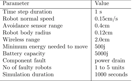
Table 2: Robot fixed parameters for all simulations.

Parameter Value

Time step duration 1 s

Robot normal speed 0.15cm/s

Avoidance sensor range 0.4cm

Robot body radius 0.12cm

Wireless range 2.0cm

Minimum energy needed to move 500j

Battery capacity 5000j

Component fault power drain

No of faulty robots 1 to 5 units

Simulation duration 1000 seconds

to robots: for a single robot failure we term it RSF, for two robot failures RT F

and three or more robot failures (until 5) we term them RT M. In RSF, one

robot in the environment will experience a power reduction approximately at time=100 seconds in the simulation. For RT F, two robots will be supplied with

a power reduction simultaneously at t=100 seconds whilst with RM F, three and

more failing robots will be introduced simultaneously in the simulation. During this time, the robots are not moving and will remain static in the environment. The parameter for the faulty scenario is shown in Table 3.

Table 3: Variable parameters for failing scenario in the environment

Number of faults Parameter Time (s)

Single failure Speed=0 m/s, energy=500 joules t=[100] Multiple failure Speed=0 m/s, energy=500 joules t=[100]

In these experiments we measure the progression of the centroid of the swarm towards the beacon for every 100 seconds, using equation 1; wherexand yare the coordinates of the robots andn is the number of robots in the experiment.

Centroid distance of robots to beacon =

n X

i=1 p

(x1i x2i)2+ (y1i y2i)2

3.2. Results and Analysis 3.2.1. Experiment I:!-algorithm

H10: The use of!-algorithm (M1) for swarm beacon taxis allows the swarm to achieve a centroid distance less than 5 cm away from the beacon when there are no failures introduced.

H20: The use of !-algorithm (M1) for swarm beacon taxis allows all robots in the swarm to achieve the distance less than 5 cm away from the beacon with a completely failed robot in the environment.

H30: The use of !-algorithm (M1) for swarm beacon taxis allows all robots in the swarm to achieve the distance less than 5 cm away from the beacon with more than two failing robots in the environment.

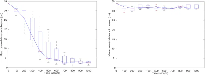
Our experiment starts with the investigation of!-algorithm for swarm bea-con taxis, in e↵ect H10 as undertaken by [3]. The swarm starts in one part of the arena and moves toward the beacon. The distance from the centroid of the swarm to the beacon for each run is given in Figure 3. For each experiment the robots have a di↵erent starting position in the arena, but as the importance here is on the relative performance between di↵erent sets of runs, the starting point was set to 35 cm from the beacon. This allows for a comparison between each run, as comparison between runs will be for identical starting distances from the beacon. The hypothesis can be accepted if the swarm centroid comes close to the beacon within a range of less than 5 cm. Based on the experiments, the swarm has a mean of velocity of 1.2 cm/simulation seconds. The fastest in the experiment of 10 robots moved at 1.52 cm/simulation seconds and the slowest had the velocity of 1.01 cm/simulation seconds. At time t=600 seconds, swarm has reached 5 cm away from the beacon. We then use the sample data to construct a 95% confidence interval for the mean centroid position of the robots from the beacon (assumed normal) and we obtained 95% confidence interval in our experiment.

In the context of the scenario above, we then introduced a partial failure to an individual robot in the swarm, to test H20. The swarm will experience a temporary slow down as it is attempting to avoid the obstructing robots, then it will pick up its normal velocity once the failed robot has been avoided. The mean distance over time in the ten runs is shown in figure 4. The swarm has the mean velocity of 1.32cm/sec, where the fastest velocity in the experiment is 1.65 cm/sec when the swarm is trying to free itself from the failed robot. During the faulty scenario, the robot does not move and remains static. The experiment accept the hypothesis H20 at the default of ↵= 0.05 significance level, which is indicated by the pvalue = 0.6442 is much greater than the ↵. The 95% confidence interval on the mean centroid distance of robots to the beacon is less than 5cmis obtained from this experiment.

Figure 3: Boxplots of the distance between swarm centroid and beacon as a function of time for 10 experiments using!-algorithm with no robot failure for H10. The centre line of the

box is the median while the upper edge of the box is the 3rd_{quartile and the lower edge of}

the box is the 1st_{quartile. At about t=600 seconds, the swarm has reached the beacon}

Figure 4: Boxplots of the distance between swarm centroid and beacon as a function of time for 10 experiments using!-algorithm with one robot fails at t=100 seconds for H20. The

centre line of the box is the median while the upper edge of the box is the 3rd_{quartile and}

the lower edge of the box is the 1st_{quartile. The swarm reach the beacon at t=700 seconds}

able to reach less than 5cmaway from the beacon when two failing robots are introduced to the system, the anchoring problem will manifest as three failing robots are introduced to the systems. With three failed robots, the experiment reject the hypothesis H30 at the default of↵= 0.05 significance level, which is indicated by the p value = 3.6926e-14 that has fallen below the ↵. The 95% confidence interval on the mean centroid distance of robots to the beacon is more than 5cm is obtained from this experiment.

(a) Boxplots of the distance between swarm centroid and beacon as a func-tion of time for 10 experiments using! -algorithm with two robot fails simulte-nously at t=100 seconds for H20. The

centre line of the box is the median while the upper edge of the box is the 3rd

quar-tile and the lower edge of the box is the 1st_{quartile. The swarm reach the beacon}

at t=850 seconds

(b) Boxplots of the distance between swarm centroid and beacon as a func-tion of time for 10 experiments using! -algorithm with three robot fails simulta-neously at t=100 seconds H30. The

cen-tre line of the box is the median while the upper edge of the box is the 3rd_quartile

and the lower edge of the box is the 1st

quartile. The swarm does not reach the beacon as the failing robots anchor the swarm

Figure 5: The!-algorithm with two and three failing robots

Results from the experiments show that, even with two completely failed robots the swarm will always reach the beacon, and the delay is once again relatively small. However, as three faulty robots are introduced in the simula-tion, the swarm starts to show a complete halt, not reaching the beacon and stagnate around the three failing robots as shown in figure 5(b). This confirms the potential issue of “anchoring” in swarm beacon taxis that is described in section 2.1. From all experiments that have been conducted, we have confirmed the observations of [3] that the anchoring issue, occur in the swarm beacon taxis as more failures are injected in the systems. The failing robot will ‘anchor’ the swarm impeding its movement towards the beacon.

charger algorithms.

3.2.2. Experiment II: Single Nearest Charger Algorithm

H40: The use of single nearest charger mechanism (M2) for swarm beacon taxis does not improve the ability of the robots in the systems to reach the beacon when compared with M1 when more than two faulty robots are introduced to the systems

As discussed by [9], in contrast of the form of ‘central sharing’, robots must be able to distribute the collective energy resources owned by the group member (trophallaxis). Taking this idea, we apply a simple solution in energy sharing between robots in the simulation called the single nearest charger algorithm. We begin by assuming the simplest rules basically depend on the each robot’s position in the environment. We limit the energy transfer between two robots, meaning that each robot can only receive or donate energy from one robot at any one time [9]. We also constrain the system such that the nearest robot that acts as the donor cannot reject the request and must donate the amount of energy defined by the energy threshold in the simulation. In our experiment, we set the energy threshold = 1500 Joules, thus each donor can only transfer the up to the energy threshold to preserve the donor’s energy. This algorithm is outlined in algorithm 1.

This experiment tests hypothesis H40 to determine whether better results can be obtained from a single charger algorithm that is described in algorithm 1. Thus, the first experiment tests whether the single charger algorithm is able to allow the systems to move at least 5cm away from the beacon with failing robots in the environment.

begin

Deployment: robots are deployed in the environment

repeat

Random movement of the robot in the environment Signal propagation: Faulty robots will emit faulty signal Rescue: One of the healthy robots with the nearest distance (earliest arriving robot) will perform protection and rescue Repair: Sharing of energy between faulty and healthy robots according to algorithm 2

untilforever

end

Algorithm 1: Overview of single nearest charger algorithm

Algorithm 1 reflects the overview of single nearest charger algorithm to do the repair for the faulty robot(s). The basic terms used in the algorithm are outlined below:

• posself(t): position of the current robot

begin

Evaluate posself(t) Send posself(t)to peers

Receiveegypeer(t x) andposself(t x)from peers

forall egypeer(t x)do

Evaluate egypeer(t x)

if egypeer(t x)< egymin then

Evaluatepospeer(t x)

Sortpospeer(t x)in ascending order Move to nearestpospeer(t x)

else

Do not move topospeer(t x)

end end end

Algorithm 2: Algorithm for containment and repair for single nearest charger algorithm

• egyself(t): energy of the current robot • egypeer(t x): energy of peer robots

• egymin: minimum energy required • egyneeded: energy needed by each robot

Similar to the previous set of experiments in M1 (our baseline), M2 is tested with the same scenarios and results are compared to M1. We look at both statistical and scientific significance. Statistical significance is measured with ranksum test and scientific significance with A measure [21]. The interpreta-tion of A value is such that a value around 0.5=no e↵ect, 0.56=small e↵ect, 0.64=medium e↵ect, and 0.71=big e↵ect. A p value of 0.05 for ranksum test is commonly used to signify that two samples are di↵erent with the statistical significance because the medians are di↵erent at a 95% confidence level.

In the first experiment with RSF and RT F, M2 does not di↵er greatly

from M1 which is indicated by the p value=0.54 with one robot fails and p value=0.8150 with two robots fail. From this results the swarm can get within 5 cm of the beacon. However, as compared to M1, in M2 all robots are able to arrive to the beacon whereby in M1, even though with one and two failing robots in the swarm, the swarm can reach the beacon but they leave the failing robots behind and avoid them as obstacles: this is consistent with the observa-tions by [3] and [2] as discussed in Section 2.1. The results for M2 for one and two failing robots are shown in figure 6(a) and 6(b).

and four failed robots in the system. Results for three and four failing robots are shown in figure 6(c) and figure 6(d). For five failed robots M2 does not gives a better performance if compared with M1 as indicated by thepvalue = 0.3033. The di↵erence between M2 and M1 is shown in table 4. Therefore, with three and four failed robots, the experiments reject the hypothesis H40 with 95% confidence level on the mean centroid distance of the robots to the beacon is more than 5cm is obtained.

Table 4: P and A value for mean centroid distance on robots between M1 and M2 in 1000 simulation seconds.

M2/M1 ranksum P A measure

One fail 0.54 0.7908

Two fails 0.8150 0.0181

Three fails 1.7661e-04 1

Four fails 1.7562e-04 1

Five fails 0.3033 0.640

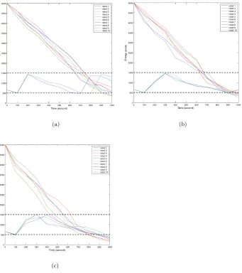
The robots start with same levels of energy which is 5000 Joules. In each failing case, the energy is reduced as explained in table 3. The threshold value for the failing robots to start triggering failing signal is 500 J. Figure 7(a), 7(b) and 7(c) show the energy of each robot during 1000 simulation seconds with di↵erent failing robots in the environment. In figure7(b), three failing robots are introduced into the environment. Half of the swarm reach the minimum energy threshold in 900 simulation. From figure 7(c) we can see that for four failing robots, the swarm starts to reach the minimum energy threshold dur-ing 900 simulation seconds. This trend continues for five faildur-ing robots in the environment.

In summary, results from this experiment show that M2 performs slightly better than M1 but the swarm cannot reach the beacon if the number of failing robots is more than three. During the experiments, we also observe that the nearest charging robot may not have sufficient energy to donate to the faulty robots leading to the failure of the charging robots. This method would also be applicable if the number of failing unit is small (less than half of the swarm fails). However as more robots fail, they will then act as ‘anchor’ the swarm leading to impeding the swarm to moves towards the beacon. Although M2 managed to achieve desirable solution with RSF and RT F but, for RM F, is unable to reach

the beacon in all simulated scenarios. Thus, the next set of experiments in the following section investigates an enhanced method and introduces the shared nearest charger mechanism.

3.2.3. Experiment III: Shared Nearest Charger Algorithm

(a) (b)

(c) (d)

Figure 6: Boxplots of the distance between swarm centroid and beacon as a function of time for 10 experiments using single nearest charger algorithm with one faulty robot (6(a)), two robots fail simultenously at t=100 seconds(6(b)), three robots fail simultenously at t=100 seconds (6(c)) and four robots fail simultenously at t=100 seconds (6(d)). The centre line of the box is the median while the upper edge of the box is the 3rd _{quartile and the lower}

edge of the box is the 1st_{quartile. In figure 6(a), with one faulty robot, the swarm reach the}

beacon at t=650 seconds. With two failing robots in figure 6(b), the swarm reach the beacon at t=900 seconds. Meanwhile as depicted in figure 6(c) and figure 6(d) the swarm does not reach the beacon as the failing robots ‘anchor’ the swarm to moves towards the beacon.

Here we investigate whether M3 with a shared charger mechanism can out-perform M2 and M1 with a mean centroid distance of robots from the beacon is 5cm. Based on the idea of single nearest charging, we extend the algorithm by increasing the number of donors to each faulty robot. The general algorithm of shared nearest neighbour algorithm is presented in algorithm 3, which is also illustrated in figure 8.

(a) (b)

(c)

begin

Deployment: robots are deployed in the environment

repeat

Random movement of the robot in the environment Signal propagation: Faulty robots will emit faulty signal Rescue: n number healthy robots with the nearest distance (earliest arriving robot) and highest energy will perform protection and rescue according to algorithm 4

Repair: Sharing of energy between faulty and healthy robots according to algorithm 2

untilforever

end

Algorithm 3: Overview of Shared Nearest Charger Algorithm

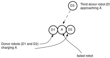
with the failed robot. In this algorithm, the robots can transfer the minimum amount of energy from each of the neighbouring/charging robots taking into account that priority will be given to the robots with higher energy and near to the failing robots. In the algorithm, we limit the energy transfer between three robots, which means that each faulty robot can only receive energy simultaneous from three nearest robots. The donor must donate the amount of energy defined by the energy transfer rule in algorithm 4.

Figure 8: The illustration of shared nearest charger algorithm

The basic terms used in the algorithm are as follow:

• posself(t): position of current robot • pospeer(t x): position of peer robots

• egyself(t): energy of current robot

• egypeer(t x): energy of peer robots

• egymin: minimum energy required

begin

Evaluate posself(t) Send posself(t)to peers

Receiveegypeer(t x)/ andposself(t x)from peers

forall egypeer(t x)do

Evaluate egyneeded(t) Divide egyneeded(t) with n Sendegyneeded(t)to peers

if egypeer(t x)< egymin then

Evaluatepospeer(t x)

Sortpospeer(t x)in ascending order Move to nearestpospeer(t x)

else

Do not move topospeer(t x)

end end end

Algorithm 4: Algorithm for containment and repair according to energy and position of robots

• n: number of donor robot, in this experiment n = 3

As with previous experiments in section 3.2.1 and section 3.2.2, M3 is tested in the same scenarios and results compared to M2 and M1. We again look at both statistical and scientific significance.

In the first experiment with RSF and RT F, results of M3 do not di↵er greatly

from M1 as in both methods, the swarm cannot reach the beacon if the number of failing robots is more than three. However, as compared to M1, in M2 all robots are able to arrive at the beacon. The results for M3 are shown in figure 9(a), 9(b), 9(c) and 9(d). Based on figure 9(a) and figure 9(b), M3 works well with one and two failing robots in the systems where the swarm can reach the beacon. However, it starts to su↵er when the number of failures increases. With three, four and five failing robots in the system, the swarm fails to reach the beacon. These are shown in figure 9(c) and figure 9(d). In the experiment with RSF and RT F, results of M3 do not di↵er much from M1 and M2 as in all

methods, all robots in the swarm can reach the beacon. These are illustrated in figure 9(a) and figure 9(b). However, this algorithm is unable to perform the task in reaching the beacon with RM F. As depicted in figure 9(c) and figure

9(d), they can only reach around 10 to 15cm away from the beacon. We will later describe the significance di↵erences between M3, M2 and M1.

Both algorithms do not di↵er statistically with RSF and RT F but, for RM F,

fails the remaining robots are not able to reach the beacon. This scenario is observed during simulation M1 and M2 for swarm beacon taxis, and again is consistent with similar observations by [2].

Table 5: P and A value for mean centroid distance on robots between M3 and M2 in 1000 simulation seconds.

M3/M2 ranksum P A measure

One fail 0.3631 0.3750

Two fails 0.2404 0.34

Three fails 0.4261 0.6100

Four fails 0.0930 0.7200

Five fails 0.8785 0.4750

M3 and M1, do not di↵er statistically with RSF and RT F but, with three and

four failing robots in the system, the experiment reject the hypothesis H50at the default of↵= 0.05 significance level, which is indicated by thepvalue = 1.7462e-04 andpvalue = 1.0650e-04 that have fallen below the ↵. Thus, M3 performs significantly better from M1 when there are three and four failing robots in the system. For five failing robots M3 does not gives a better performance if compared with M1 as indicated by thepvalue = 0.4226. The di↵erence between M3 and M1 is shown in table 6. Therefore, with three and four failing robots, the experiments reject the hypothesis H40 with 95% confidence level on the mean centroid distance of the robots to the beacon is more than 5cm .

Table 6: P and A value for mean centroid distance on robots between M3 and M1 in 1000 simulation seconds.

M3/M1 ranksum P A measure

One fail 0.650 0.2718

Two fails 0.57 0.62

Three fails 1.7462e-04 1

Four fails 1.0650e-04 1

Five fails 0.4226 0.61

the swarms only reach around 10 to 15cm from the beacon when they move around the failed robots. This trend again continues for 5 failing robots in the environment.

3.3. Experimental Findings

So far, we have studied the e↵ect of single nearest charger and shared nearest charger algorithms in an attempt to resolve the potential anchoring issues for power failure in the context of swarm beacon taxis. Based on these results, we observe issues with swarm taxis in line with [2] and with simple repair strate-gies are unable to mitigate these issues. With asingle nearest charger algorithm, only one robot needs to share its energy with a faulty robot. However, since only one robot is sharing the energy, it has to give a large proportion of the required energy to the faulty robot, resulting to the major reduction on its own energy. This issue is crucial, and potentially not scalable, when the number of faulty robots increases. In an attempt to resolve this issue, we proposed an enhance-ment by increasing the number of simultaneous chargers . Here, we proposed a shared nearest charger algorithm, with three charging robots for each failing robot in the environment. Compared with thesingle nearest charger algorithm, the robots will no longer su↵er with major energy reduction. However, when too many robots try to reach the faulty robots, docking and navigation is clearly an issue as robots interfere with each other to recharge the failing robots. Thus, a design of the docking and signalling algorithms than can improve the navigation is clearly needed. Due to these issues, we propose an immune-inspired solution inspired by the process of granuloma formation in immune systems. In the re-maining part of the paper, we first describe the process granuloma formation in section 4. Secondly, we explain the computational model of granuloma forma-tion in accordance with the idea of immuno-engineering as proposed in [19] in section 4.1 and finally we describe the granuloma formation algorithm in section 4.2, followed by an empirical investigation into the algorithms performance.

4. Granuloma Formation

An immune system is a complex system, involved in the defence of a host that has evolved in animals and plants over millions of years. There are many threats to hosts, and the immune system has evolved a variety of mechanisms to cope with these threats [18]. Of particular interest to our work is the formation of structures known as granulomain response to certain pathogenic infection. Granulomas form in response to cells being infected by pathogens (in particular in response to infection by tuberculosis and Leishmanianas), and are structures that form of particular immune cells, known as T-cells that try and contain the infection in the cell and prevent cell to cell transmission of the pathogen [14]. The main cells involved in granuloma formation are; macrophages, T-cells and cytokines. [14] outline three main stages of granuloma formation:

2. Cytokines and chemokines are released by macrophages, activated T-cells and dendritic cells. The released cytokines and chemokines attract and retain specific cell populations.

3. The stable and dynamic accumulation of cells and the formation of the organised structure of the granuloma.

These do vary slightly depending on location of the formation, be that in the liver or lung, for example, but the principles are the same.

In granuloma formation a cell called a macrophage will ‘eat’ or engulf the pathogen in an attempt to prevent the pathogen from spreading. However, the pathogen may infect the macrophage and begin to duplicate. Therefore, despite the fact that macrophages are able to stop the infection, pathogens will use macrophages as a‘taxi’ to spread diseases leading to the cell lysis (the breaking down the structure of the cell). Infected macrophages then will emit a signal which indicates that they have been infected and this signal will lead other macrophages to move to the site of infection, to encase the infected cells, in e↵ect then isolating the infected cells from the uninfected cells. This will ultimately lead to the formation of a granuloma structure, and in many cases the removal of the pathogenic material. By separating the infected macrophages, the robustness of the system will be maintained and the failure of one or more cells will not a↵ect other cells and the overall task of the system can be maintained. During granuloma formation, macrophages form a walling around the chron-ically infected macrophages as well as the bacteria leading to the formation of granuloma with the objective of separating the infected and uninfected cells as well as separating the bacteria from the healthy cells. By separating the in-fected macrophages, the robustness of the systems will be maintained and the failure of one or more cell will not a↵ected other cell and the overall desired task of the systems can be achieved. Based on our literature survey in Section 3.1, macrophages have essentially four states:

• uninfected: able to take up bacteria (phagocyte) and if not activated quickly, it will become infected; not secreting anything

• infected: can still phagocytose and kill but function will decreases with increasing bacterial load, able to secrete chemokines

• activated: efficient at killing their intracellular bacterial load. In order to be activated, macrophages need to be activated by T-cell

• chronically infected: cannot phagocyte or kill; secrete chemokines

For our purpose, the most important property in granuloma formation is the communication between macrophages which is determined by the level of chemokine secretion. Chemokines will not only attract other macrophages to move towards the site of infection but it will activate T-cells that will secrete cytokines to act as a signal for activation of macrophages. T-cells and activated macrophages are able to kill extra cellular bacteria that will control infections in immune systems. This is show in Figure 12. In this figure, we illustrate the di↵erent stages of macrophages and shows how the secretion of chemokines at-tract other macrophages. The infected macrophage which is in blue will secrete chemokines to attract other uninfected macrophages to the site of infection so that it can be isolated from the other cells and thus prevent further infection.

It is this early stage formation that we find interesting in the case of the swarm beacon taxis failures. We propose that there is a natural analogy between the potential repair of a swarm of robots, as in the situation of swarm beacon taxis, and the formation of a granuloma and removal of pathogenic material. We now explore this analogy in the context of immuno-engineering [19].

4.1. Computational Model of Granuloma Formation

In understanding the problem domain and the immune systems under study, we follow the engineering approach that is proposed by [18]. Immuno-engineering is defined in [18] as:

‘The abstraction of immuno-ecological and immuno-informatics prin-ciples, and their adaptation and application to engineered artefacts (comprising hardware and software), so as to provide these artefacts with properties analogous to those provided to organisms by their natural immune systems. ’

Immuno-engineering involves the adoption of conceptual framework [15] in AIS algorithm development and the problem-oriented perspective described in [4]. [18] propose a bottom-up approach to the engineering of such systems which will be achieved via an interdisciplinary approach which cuts across immunology, mathematics, computer science and engineering. Having explained the problem domain in which we are working, we now are able explore the biological back-ground to our solution and take that forward towards a novel immune inspired aggregation algorithm for swarm robotic systems.

simulation, we have constructed four design principles of self-healing in swarm robotic systems. The four principles for our algorithm development are:

1. The communication between agents in the system is indirect consisting number of signals to facilitate coordination of agents.

2. Agents in the systems react to defined failure modes by means of faulty from non-faulty using self-organising manner

3. Agents must be able to learn and adapt by changing their role dynamically. 4. Agents can initiate a self-healing process dependant to their ability and

location.

As we have discussed in [20] applying the granuloma formation concepts to swarm robotics allows us to perform two related tasks. First, we may isolate faulty robots. Given that we can detect faulty robots, such robots may e↵ect the performance of other robots and act as an ‘anchor’ to other robots, as we have shown above. In [20] we discuss how we can assume that certain signals can be sent by the robot which other functional robots nearby can recognise. These functional robots are then attracted towards the faulty robot, akin to how T-cells are attracted by cytokines emitted by an infected macrophage. A limited number of these robots then isolate the fault robot, akin to T-cells surrounding an infected macrophage, but still move around the faulty robot so that other functional robots in the swarm are no longer drawn to the ‘anchor’ point that could be the faulty robot. We now move to the development of agranuloma inspiredapproach to a self-healing swarm.

4.2. Granuloma Formation Algorithm

Using our knowledge gained from the development of a computational model, and the subsequent derivation of the design principles outlined above, we have derived the granuloma formation algorithm for solving the anchoring issue in swarm beacon taxis. We illustrate the process of granuloma formation algorithm in figure 13 which then is outlined in algorithm 5. The key di↵erences between the granuloma formation algorithm and the shared charger algorithm is the number of functional robots that will surround and share the energy with the faulty robots varies, it is not pre-defined. This will be explained later.

As outlined in algorithm 5, in granuloma formation, failing robots will send signals that can be recognised by other functional robots. These functional robots are then attracted towards the faulty robot, akin to how T-cells are attracted by cytokines emitted by an infected macrophage in granuloma forma-tion. A limited number of these robots then isolate the faulty robot, akin to T-cells surrounding an infected macrophage. The other robots which are not in-volved in isolating the faulty robot will ignore the failing and surrounding robots and treat them as if they were obstacles in a manner similar to the standard !-algorithm.

begin

Deployment: robots are deployed in the environment

repeat

Random movement of the robot in the environment

Signal propagation: Faulty robots will emit faulty signal, where the average radius of the target neighbouring robot is R

Protection and rescue: Healthy robots will decide how many will perform protection and rescue according to algorithm 6

Repair: Sharing of energy between faulty and healthy robots according to algorithm 7

untilforever

end

Algorithm 5: Overview of Granuloma Formation Algorithm

to repair the failing robot, together with the location of the faulty robot. Each faulty robot is able to evaluate their own energy level and position, and propa-gate that information to other robots, as outlined in algorithm 6. An illustration for this process is shown in figure 14. From this figure, when there exists a faulty robot(s), it will emit a signal to robots at a certain predefined radius (R). The robots that receive the signal will communicate, exchanging the information on their locations and their current energy. This is according to the energy transfer rules explain in algorithm 7, where the nearest functional robot will come alongside the robot, and share an amount of energy. If the energy that can be donated by the nearest functional robot is enough the faulty robots will stop sending the information to the other robots. However, if the energy is not enough, the faulty robot will continue to request energy from other functional robots in the environment. This will be repeated until enough energy infor-mation is obtained and then the isolating and sharing of energy will then take place.

begin

Evaluate egyneeded(t)

Send egyneeded(t)to peers withinR

Receiveegypeer(t x) from peers withinR

forall egypeer(t x)received do

if egypeer(t x)received< egyneeded then

Sendegyneeded(t)to peers withinR

else

Stop sendingegyneeded(t) to peers withinR

end end end

Algorithm 6: Algorithm for containment and repair according to energy and position of robots

begin

Evaluate egyself(t)andposself(t)

Send egyself(t)andposself(t)to peers withinR

Receiveegypeer(t x) andpospeer(t x)from peers

forall egypeer(t x)received do if egypeer(t x)< egymin then

R = matchegypeer(t x),egyself(t) Storeegypeer(t x) in inbound queue

else

R’ = not matchegypeer(t x),egyself(t) Addegypeer(t x)to outbound queue

end end

forall egypeer(t x)in inbound queue do

Add signature

Store egypeer(t x)in robot list

forall egypeer(t x)in robot list do if egyself(t)< egythresholdthen

Evaluatepospeer(t x)

Sortpospeer(t x)in ascending order Move to nearestpospeer(t x)

end end end

forall egypeer(t x)in outbound queue do

Delete signature

end end

• posself(t): position of self robot • pospeer(t x): position of peer robots

• egyself(t): energy of self robot

• egypeer(t x): energy of peer robots

• egyneeded: energy needed by failing robot

• egythreshold: the limit of the energy that is needed

In the real robot scenario, during the repairing phase, donor robots will share their energy with the faulty robots. During this time, we will adopt the ideas of signalling mechansim in granuloma formation that is explain in section 4. In granuloma formation, di↵erent signals are emitted by macrophages to inform other cells their current status. In granuloma formation algorithm, we will use di↵erent color of LED signals during the repairing phase. The green LED signals will be emitted by the faulty and donor robots that are involved in this phase notifying the other robots to ignore them and continue moving towards the beacon. This is illustrated in figure 15.

4.3. Experimental Investigation to the Granuloma Formation Algorithm For this experiment, we follow the experimental protocol that is described in Section 3.1. We cast our hypotheses as follows:

H60: The use of a granuloma formation algorithm (M4) does not improve the ability of the robots in the system to reach the beacon when compared to M2 when more than two faulty robots are introduced to the systems

H70: The use of a granuloma formation algorithm (M4) does not improve the ability of the robots in the system to reach the beacon when compared to M3 when more than two faulty robots are introduced to the systems

This experiment tests hypothesis H60and H70to determine the performance of the granuloma formation algorithm. The first set of experiments are on swarm beacon taxis with RSF and RT F. We than continue to test the algorithm with

RM F. M4 is assessed with the same scenario as the single nearest charger

algorithm (M2), shared charger algorithm (M3) and!-algorithm (M1) as the base line experiments. We than compare the algorithms and examine at the statistical and scientific di↵erences with ranksum and A measure tests. Results for M4 are illustrated in figure 16(a), 16(b), 16(c) and 16(d). Based on the graphs, swarm beacon taxis with M4 is able to reach the beacon with RSF,

RT F and RM F.

We now measure the significant di↵erence between M4 with single nearest charger algorithm (M2) and shared charger algorithm (M3). We also compare M4 with!-algorithm (M1). All results are shown in table 7 and table 8. With RSF, RT F, there is no significant di↵erence between M4, M3 and M2. This

Table 7: P and A value for mean centroid distance on robots between M4 and M3 in 1000 simulation seconds.

M4/M2 ranksum P A measure

One fail 0.7903 0.4600

Two fails 0.4722 0.4000

Three fails 0.0350 0.8900

Four fails 1.0650e-04 1

Five fails 1.7861e-04 1

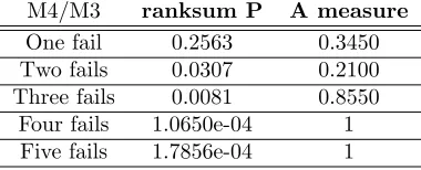
Table 8: P and A value for mean centroid distance on robots between M4 and M2 in 1000 simulation seconds.

M4/M3 ranksum P A measure

One fail 0.2563 0.3450

Two fails 0.0307 0.2100

Three fails 0.0081 0.8550

Four fails 1.0650e-04 1

Five fails 1.7856e-04 1

of the mechanisms is able to make the systems recover and operate to perform the needed task. The crucial part is when there are three or more robots that fail. The algorithm must cater for this type of failure to achieve robustness. If we compare M4 with M3 and M2 with RM F, it shows that M4 performs

significantly better than M3 and M2 with 3, 4 and 5 failing robots. M4 also performs better than the baseline experiment in this paper.

Form these experiments, even though M4 does not di↵er significantly with M2 and M3 with less than one and two failing robots, with three, four and five failing robots, the experiments reject the hypothesis H60 at the default of ↵= 0.05 significance level, which is indicated by the pvalue = 0.0350,p value = 1.0650e-04 andp value = 1.7861e-04 that has fallen below the↵. The 95% confidence interval on the mean centroid distance of robots to the beacon is less than 5 cm is obtained from this experiment. The experiments also reject the hypothesis H70 at the default of↵= 0.05 significance level with more than two failing robots are introduced to the system, which is indicated by the p value = 0.0081,pvalue = 1.0650e-04 andpvalue = 1.7856e-04 that has fallen below the↵. The 95% confidence interval on the mean centroid distance of robots to the beacon is less than 5cmis obtained from this experiment.

levels. The swarm is able to continue operating even with such failures.

5. Conclusion

References References

[1] Bayindir L, S¸ahin E (2007) A review of studies in swarm robotics. Turkish Journal of Electrical Engineering and Computer Science 15(2):115–147

[2] Bjerknes J, Winfield A (2010) On fault-tolerance and scalability of swarm robotic systems. In: Proc. Distributed Autonomous Robotic Systems (DARS)

[3] Bjerknes JD (2009) Scaling and fault tolerance in self-organized swarms of mobile robots. PhD thesis, University of the West of England, Bristol, UK.

[4] Freitas A, Timmis J (2007) Revisiting the foundations of artificial immune systems for data mining. IEEE Transaction on Evolutionary Computation 11(4):521–540

[5] Gerkey B, Vaughan RT, Howard A (2003) The player/stage project: Tools for multi-robot and distributed sensor systems. In: Proceedings of the 11th International Conference on Advanced Robotics (ICAR 2003), pp 317–323

[6] Haek MA, Ismail AR, Basalib AOA, Makarim N (2015) Exploring energy charging problem in swarm robotic systems using foraging simulation. Ju-rnal Teknologi 76 (1):239–244

[7] Ismail AR, Timmis J (2010) Towards self-healing swarm robotic systems inspired by granuloma formation. In: Special Session: Complex Systems Modelling and Simulation, part of ICECCS 2010, IEEE, pp 313 – 314

[8] Melhuish C, Hoddell OHS (1998) Collective sorting and segregation in robots with minimal sensing. In: Proceedings of the fifth international con-ference on simulation of adaptive behavior on From animals to animats 5, MIT Press, pp 465–470

[9] Melhuish C, Kubo M (2007) Collective energy distribution: Maintaining the energy balance in distributed autonomous robots using trophallaxis. In: Alami R, Chatila R, Asama H (eds) Distributed Autonomous Robotic Systems 6, Springer Japan, pp 275–284

[10] Mondada F, Bonani M, Raemy X, Pugh J, Cianci C, Klaptocz A, Magnenat S, Zu↵erey JC, Floreano D, Martinoli A (2009) The e-puck, a Robot De-signed for Education in Engineering. In: Proceedings of the 9th Conference on Autonomous Robot Systems and Competitions, vol 1, pp 59–65

[12] Ohkura K, Yu T, Yasuda T, Matsumura Y, Goka M (2015) Robust swarm robotics system using cma-neuroes with incremental evolution. Interna-tional Journal of Swarm Intelligence and Evolutionary Computation 4 (125):1–10

[13] S¸ahin E (2005) Swarm robotics: From sources of inspiration to domains of application. In: International Workshop of Swarm Robotics (WS 2004), Springer, LNCS, vol 43, pp 10–20

[14] Sneller MCM (2002) Granuloma formation, implications for the pathogen-esis of vasculitis. Cleveland Clinic Journal of Medicine 69(2):40–43

[15] Stepney S, Smith R, Timmis J, Tyrell A, Neal MJ, Hone ANW (2005) Conceptual framework for artificial immune systems. Unconventional Com-puting 1(3):315–338

[16] Støy K (2001) Using situated communication in distributed autonomous mobile robotics. In: In Proceedings of the 7th Scandinavian conference on artificial intelligence, Amsterdam: IOS, pp 44–52

[17] Støy K, Shen WM, Will P (2002) Global locomotion from local interaction in self-reconfigurable robots. In: 7th International Conference on Intelligent and Autonomous Systems (IAS7), pp 309–316

[18] Timmis J, Andrews P, Owens N, Clark E (2008) An interdisciplinary per-spective on artificial immune system. Evolutionary Intelligence 1(1):5–26

[19] Timmis J, Hart E, Hone A, Neal M, Robins A, Stepney S, Tyrrell A (2008) Immuno-engineering. In: 2nd International Conference on Biologically In-spired Collaborative Computing, IFIP, vol 268, pp 3–17

[20] Timmis J, Tyrrell A, Mokhtar M, Ismail AR, Owens N, Bi R (2010) An artificial immune system for robot organisms. In: Levi P, Kernback S (eds) Symbiotic Multi-Robot Organisms: Reliability, Adaptability and Evolu-tion, vol 7, Springer, pp 279–302

(a) (b)

(c) (d)

(e)

(a) (b)

(c) (d)

a) Movement b) Infected cells

c) Signal propagation d) Granuloma formation

Figure 11: Simple scenario: formation of granuloma

Signal propagation . . . . . . . . .._{. .} . . . ... . . .._. . . . . .._. . . .. . .. . . . . . .. ._. . . . . . . . . . . .._. . . .. . . . . ..._... . . . . . . . . .. . . . . . . . . . . . . . . . .._. . . . .._. . . .. . . . . ... . ._. . ._... . ._..... . ... . . . ... . . . ..._.._.. .. _.._.. . . . . . .. . . .. . . . ... ... ._. . ._.... ... . . .. . .._. . .. . ._.. . . .. ._.. . . ... ... . ... . . .. . . . . . ._{.. .. .} . . . . . . . . .. . . . . . . . . . ._. . .. . . .. . . .. . .. . . .. . . ._. . .. . . .. . . . . . . . . . . . . .. . . . . . ... ... . ... .._.... . .. . . . . . ... ... . ... .._.... . .. . . . . . ... ... . ... .._.... . .. . . . . . ... ... . ... .._.... .. . . . . . ... ... . ... .._.... . .. . . . . . ... ... . ... ... .

Figure 13: Simple Scenario: granuloma formation algorithm

(a) (b)

(c) (d)

(e)

Figure 16: Boxplots of the distance between swarm centroid and beacon as a function of time for 10 experiments using granuloma formation algorithm with one faulty robot (16(a)), two failing robots (16(b)), three failing robots (16(c)), four failing robots (16(d)) and five failing robots (16(e)) simultenously at t=100 seconds, for H60and H70. The centre line of the box

is the median while the upper edge of the box is the 3rd _{quartile and the lower edge of the}

box is the 1st_{quartile. The swarm reach the beacon at t=650 for one faulty robot, at t=800}

(a) (b)

(c)