Computational grid generation for the design of free-form shells with
complex boundary conditions
Tierui Li1, Jun Ye2, Paul Shepherd3, Boqing Gao5
1 PhD Student, College of Civil Engineering and Architecture, Zhejiang University, Hangzhou, 310058. Email:
2 Research Associate, Dept. of Architecture & Civil Engineering, Univ. of Bath, Bath, BA2 7AY. Email: [email protected]. 3 Associate Professor, Dept. of Architecture & Civil Engineering, Univ. of Bath, Bath, BA2 7AY. Email: [email protected].
4 Professor, College of Civil Engineering and Architecture, Zhejiang University, Hangzhou, 310058.Email: [email protected].
Abstract: Free-form grid structures have been widely used in various public buildings, and many are bounded by complex curves including internal voids. Modern computational design software enables the rapid creation and exploration of such complex surface geometries for architectural design, but the resulting shapes lack an obvious way for engineers to create a discrete structural grid to support the surface that manifest the architect’s intent. This paper presents an efficient design approach for the synthesis of free-form grid structures based on “guide line” and “surface flattening” methods, which consider complex features and internal boundaries. The method employs a fast and straightforward approach, which achieves fluent lines with bars of balanced length. The parametric domain of a complete NURBS (Non-Uniform Rational B-Spline) surface is firstly divided into a number of patches, and a discrete free-form surface formed by
mapping dividing points onto the surface.The free-form surface was then flattened based on the principle of equal area. Accordingly, the flattened rectangular lattices are then fit to the 2D surface, with grids formed by applying a guide-line method. Subsequently, the intersections of the guide-lines and the complex boundary are obtained, and the guide-lines divided equally between boundaries to produce grids connected at the dividing points. Finally, the 2D grids are mapped back onto the 3D surface and a spring-mass relaxation method is employed to further improve the smoothness of the resulting grids. The paper concludes by presenting realistic examples to demonstrate the practical effectiveness of the proposed method.
Introduction
Gridshells as long spanning roof structures are often the most striking part of such a building. They provide a sense of simplicity and elegance in terms of appearance. Their important features are their uninterrupted span, the smoothness of their continuous surface, the sparseness of their structural grid, curve fluidity and most importantly their high structural efficiency that can resist external actions through membrane stiffness (Malek and Williams 2017). Gridshells with multi-planar, cylindrical, spherical and parabolic shapes are not uncommon in practice (Kang et al., 2003; Shilin, 2010; Cui and Jiang, 2014), where engineers use analytical equations to generate nodal positions and member connectivity, as shown in Fig.1.
Fig.1Free-form grid structures: the British Museum Great Court
In general, however, free-form surfaces cannot be expressed accurately by means of (piecewise) analytic functions, and the curvature of such surfaces is generally complex. In recent years, parametric modeling techniques in computer aided design (CAD) have brought a new level of sophistication to the generation of 3D free-form surfaces, allowing architects more freedom to create inspiring designs and to restructure their approach to design. The aesthetically pleasing nature of such designs also attracts the attention of high-profile clients and the number of new and complex free-form grid structures is increasing. Despite these advancements in CAD technology, given the varying curvature and complex boundaries associated with such designs, it remains a challenge for architects and engineers to generate structural or cladding grids on such surfaces, and the digital tools available for such tasks lag behind those available for the initial surface generation.
The grid patterns on free-form shells are traditionally created by hand using computer-aided design tools, or
a structural grid on a given free-form surface are urgently needed to facilitate the design process, particularly in the early stage. Such tools need to deliver in four key areas. Grids generated should be an approximation of the given surface. Grid members should all be of similar lengths to ease manufacture, connections, and equalize their buckling strengths and each continuous member should pass over the surface in a fluid manner
and avoid singularities of curvature (kinks), as shown in Fig.2. Finally, tools should be relatively automated and quick to run on a broad range of complex surfaces to allow the user the ability to interactively explore appealing options.
Fig.2 Gridshell with curve fluidity and regular grid cells.
One area of research where such qualities have been investigated is in the field of Finite Element Analysis (FEA). Methods such as the Advancing Front Technique (Aubry et al., 2011), the Mapping Method (Hannaby, 1988) and Delaunay Triangulation (Muylle et al., 2002; Liu et al., 2011) have been developed to generate triangular or quadrilateral meshes on complex surfaces, and the qualities needed for FEA share many characteristics with those needed for gridshells. However the resulting FEA mesh does not necessarily meet the requirement of equal rod length and certainly the architectural grid fluidity is not considered.
Grid generation methodologies specifically for free-form surfaces are therefore beginning to attract the attention of researchers. One of the earliest methods for grid generation on a 3D surface, known as the Chebyshev net, was proposed in 1878 (Popov 2002). Two arbitrary intersecting curves are first defined on a given surface, and each curve is then divided into segments of the same rod length. A grid of points is then produced by intersecting two adjacent circles on the surface, where each circle has a radius equal to the rod length. Due to the nature of these intersecting circles, this method is better known as the “Compass Method”,
Curve fluidity
as shown in Fig.3. Lefevre et al. (2015) used the Compass Method to generate gridshells for instability analysis, while a method with a denser net was proposed to improve the quality of the resulting grid.
Fig.3 Compass method
Shepherd and Richens (2012) proposed the use of the Subdivision Surface method to generate grids, where an initial triangular or quadrilateral mesh is first imposed onto a free-form surface and then subdivided over a number of iterations, snapping back to the original surface at each step. Su et al. (2014) developed a grid generation procedure using the principle-stress trajectories of a surface under specific dominant load. A
modified ‘advancing front’ mesh technique was used for the grid generation, however this involved FE analysis, which required significant computational time and the fluidity and equal rod length of grid cells was not guaranteed. Others (Zheleznyakova and Surzhikov 2013, Zheleznyakova 2015) proposed a new approach for triangular grid generation based on molecular dynamics, with nodes considered as interacting particles with mass. The particles then moved within the design domain according to residual forces and damping, and once they were finally well positioned after the molecular dynamics simulation process, well-formed triangles were created using Delaunay triangulation. More recently, Douthe et al. (2017) proposed a method to generate gridshells with quadrilateral cells using two intersection curves as guide lines. A circular mesh was generated, and the duality between a circular mesh with a unique radius and a Chebyshev net was used to obtain a quadrilateral grid that considered the planarity of each cell.
The most recent method for the synthesis of free-form grid structures was proposed by Gao et al. (2017a).
fluidity. Gao et. al. (2017b) improved on the method to include a surface flattening technique, which reduced the grid shape irregularity by up to 47%.
In practice, the free-form architectural surfaces are complex, particularly with regards their non-convex boundaries and the presence of internal holes. For example, the roof surfaces in Fig.4 have internal
boundaries that are trimmed by several closed space curves.
Fig.4 Free-form grid structures with complex boundaries: Guangzhou Sports stadium (above) and Shenzhen Bay Sports Center (below)
The main limitation of the methods reviewed above is that they struggle to cope with free-form surfaces that contain such complex boundary definitions. The key advance described in this paper is, therefore, a method that combines the surface flattening technique with an improved guide-line method that can also work with complex boundaries, both internal and external. Fluidity is also guaranteed, and the resulting grids express
Descriptions of curves and surfaces
NURBS (Non-uniform rational Basis-Splines) expressions (Piegl and Tiller, 2012) are used in this paper to represent the free-form surface. NURBS are a standard method for architectural shape representation, design and data exchange when geometric information is processed by computer. They represent the arbitrary shape of a surface by adjusting their control points and knots weights to establish a relationship between a 3D surface and a 2D parametric domain, which is convenient for surface flattening and grid generation. A pth-degree NURBS curve is shown in Fig.5 and is defined by (Piegl and Tiller 2012):
ሺݑሻ ൌσసబேǡሺ௨ሻڄఠڄ
σసబேǡሺ௨ሻڄఠ (1)
where ሼܥܲሽ are the control points, ሼ߱ሽ are the weights, and ܰǡሺݑሻ are the pth-degree B-spline basis
functions which are:
ܰǡሺݑሻ ൌ ቄͳ݂݅ݑͲݐ݄݁ݎݓ݅ݏ݁ ݑ ݑାଵ
ܰǡሺݑሻ ൌ௨௨ି௨
శି௨ܰǡିଵሺݑሻ
௨శశభି௨
௨శశభି௨శభܰାଵǡିଵሺݑሻ (2) defined on the non-periodic and non-uniform knot vector:
ܷ ൌ ൝ܽǡ ǥ ǡ ܽᇣᇤᇥ ାଵ
ǡ ݑାଵǡ ǥ ǡ ݑǡ ܾǡ ǥ ǡ ܾᇣᇤᇥ ାଵ
ൡ (3)
Fig.5 Relationship between a curve and its control points
A NURBS surface (shown in Fig.6) of degree p in the u direction and degree q in the v direction is a bivariate vector-valued piecewise rational function with the following form (Piegl and Tiller 2012):
ሺݑǡ ݒሻ ൌσసబσೕసబேǡሺ௨ሻڄேೕǡሺ௩ሻڄఠǡೕڄǡೕ
where ൛ܥܲǡൟ forms a bidirectional control net, ൛߱ǡൟ are the weights, and ܰǡሺݑሻ,ܰǡሺݒሻ are the non-rational B-spline basis functions defined on the knot vectors:
ە ۖ ۔ ۖ
ۓܷ ൌ ൝ܽǡ ǥ ǡ ܽᇣᇤᇥ ାଵ
ǡ ݑାଵǡ ǥ ǡ ݑǡ ܾǡ ǥ ǡ ܾᇣᇤᇥ ାଵ
ൡ
ܸ ൌ ൝ܿǡ ǥ ǡ ܿᇣᇤᇥ ାଵ
ǡ ݒାଵǡ ǥ ǡ ݒǡ ݀ǡ ǥ ǡ ݀ᇣᇤᇥ ାଵ
ൡ
(5)
Fig.6 The relationship between a curved surface and its control points
Fig.7 Mapping from parametric domain to the NURBS surface
Surface flattening
Surface flattening is a technique that transforms a 3D surface into a planar surface, where further operations can be more easily carried out on a planar surface compared to direct operations on the 3D curved surface. This has been widely used in engineering practice, for example, to calculate and design blank-shapes in the manufacturing industry (McCartney et al., 2005). Surfaces are classified as developable or undevelopable, depending on their Gaussian curvature, with Gaussian curvature equal to zero everywhere being the necessary and sufficient condition for a developable surface (Banchoff and Lovett, 2015). Surface flattening techniques have been used in the design of membrane structures for decades, with Topping and Iványi (2008) more recently introducing a method to transform 3D strips of membrane surfaces into planes for membrane cutting pattern generation based on the dynamic relaxation algorithm. In their method, the surface flattening process does not require the strip to be developable. There are three main methods of surface flattening, geometric-, mechanical- and combined geometric and mechanical flattening (Li et al., 2005; McCartney et.
al., 2005; Wang and Tang, 2007). The authors here also use a geometric flattening method to unfold the surface, this time based on the rule of identical area due to its high efficiency and adaptability compared to the other methods (Li et al., 2005; Wang and Tang, 2007). The technique is explained using the example of a crescent-shaped surface that has been trimmed with internal holes and a complex boundary, as shown in Fig.8.
Fig.8 Trimmed crescent shape surface with complex boundary
Surface discretization
boundary lengths. A discrete free-form quad mesh is therefore generated in 3D by mapping the dividing points of the parametric domain onto the surface, as shown in Fig.9.
Fig.9 Surface discretization
Flattening of the central point and surrounding points
The central point of the surface mesh is then used to define the flattening center and is obtained by searching the center in the parameter domain of N×M grid of segments. The coordinates of unfolded plane points corresponding to the flattening center and its surrounding eight points on the surface should be firstly determined, as shown in Fig.10.
The corresponding point of the flattening center ܣ is point ߙ on the plane and is taken as the origin of the flattening plane. Suppose ɀ is the difference in the sum of internal angles around the flattening center before and after flattening. Since after flattening the points lie in a plane and their angles therefore sum to ʹɎ, ɀ can be calculated as:
ɀ ൌ ʹɎ െ ሺߙଵ ߙଶ ߙଷ ߙସሻ (6)
The value ɀ will be allocated to the 4 regions around point a0 in the same proportion as the corresponding angles on the surface. The corresponding angles on the plane after flattening can therefore be obtained from Eq.7:
ߚ ൌ ߙ ɀ ൈ ߙΤσ ߙ (7)
Now that the angles have been determined, a scale factor is needed to determine the actual coordinates of the points on the plane. Suppose the ݑ and ݒ directions have the same rate of expansion (ݐ) before and after flattening, with ݐ as defined by Eq.8:
ݐ ൌȁబభȁ
ȁబభȁൌ
ȁబమȁ
ȁబమȁൌ
ȁబయȁ
ȁబయȁൌ
ȁబరȁ
ȁబరȁ (8)
By applying the rule that the areas of triangles ᇞ ܽܽଵܽଶ, ᇞ ܽܽଶܽଷ, ᇞ ܽܽଷܽସ, ᇞ ܽܽସܽଵ after flattening should be equal to the sum of the areas of the corresponding triangles before flattening, value of ݐ is obtained:
ȁܣܣଵȁȁܣܣଶȁ ߙଵ ȁܣܣଶȁȁܣܣଷȁ ߙଶ ȁܣܣଷȁȁܣܣସȁ ߙଷ ȁܣܣସȁȁܣܣଵȁ ߙସ ൌ ݐଶሺȁܣܣଵȁȁܣܣଶȁ ߚ
ଵ ȁܣܣଶȁȁܣܣଷȁ ߚଶ ȁܣܣଷȁȁܣܣସȁ ߚଷ ȁܣܣସȁȁܣܣଵȁ ߚସሻ (9) By rearranging Eq.(9) and solving for t, this value can then be substituted into Eq.(8) to give values
forȁܽܽଵȁ,ȁܽܽଶȁ,ȁܽܽଷȁ and ȁܽܽସȁ, and therefore the coordinates of points ܽଵ,ܽଶ,ܽଷ,ܽସ can be calculated.
Finally, the principle of identical area is also used to calculate the coordinates of points ܽହ,ܽ,ܽ,଼ܽ. Taking ܽହ as an example, suppose ܧଵ,ܧଶ,ܧଷ represent the area of triangle ᇞ ܣଵܣଶܣହ,ᇞ ܣܣଵܣହ, ᇞ ܣܣଶܣହ individually. Likewise,ܵଵ,ܵଶ,ܵଷ represent the area of corresponding triangle after flattening
and ȟ represents the sum of the squares of the changes in areas before and after flattening:
ȟ ൌ σଷୀଵሺെ ሻଶ (10)
In order to minimize ȟ, the following formula is applied:
ቐ డୗ
డ௫ ൌ Ͳ
డୗ
డ௬ ൌ Ͳ
The coordinates of point ܽହ can then be obtained by solving Eq.(11) and the coordinates ofܽ,ܽ,଼ܽ can be determined in the same way.
Flattening of the whole regions
Once the surface flattening center is determined by searching the center in the parameter domain of N×M
grid of segments, the entire surface is divided into four regions and each is then flattened in sequence.
Following the flattening of ܣ and its surrounding 8 points, point ܣଵ
,
for example can then be used as a center to flatten its surrounding points according to the same principle of identical area used to flatten point ܣ. Each region is flattened by repeating the above steps in the specific order shown in Fig.11, firstlytraversing the surface in the direction A0 Æ A1 and then A0 Æ A2 on each consecutive row and column working out from A0 to the diagonally opposite corner of the region.
(a) Grid nodes of the first region flattening in a row
(b) Grid nodes of the first region flattening 14
A0 A1 A2 A5
1 2 3 4 5 6
7 8 9
10 11 12 13 15
(c) Grid nodes of all four regions flattened Fig.11The steps of grid-flattening
When the surface shown in Fig.9 is flattened using the above method, the result is as shown in Fig.12.
Fig.12 Rectangular lattices of the doubly-curved surface flattened onto the plane
Grid generation based on an improved guide-line method
After the flattening of the free-form surface, the improved guide-line method is used to generate grids in the 2D flattened domain. The guide-line method begins by considering a curve which is sketched onto the
original 3D surface by the architect and can represent the designer’s aesthetic intent. The process then covers the entire flattened surface with multiple guide-lines by advancing the predefined guide line. The fluency and regularity of the grid cells are largely determined by the advancing guide-lines.
Fig.13 The trimming boundary on the flattened 2D surface
Guide-line advancement
First the initial guide-line should be sketched on the original surface by the designer, as shown in Fig.14. This guide-line can then be directly mapped onto the flattened 2D surface, since they share the same parametric field, as shown in Fig.15.
(a) Top view (b) Perspective view
Fig.14 The initial guide-lines on the original surface
Fig.15 The initial guide line on the flattened complete surface
Eq.(1)) of the preceding guide-line by a fixed distance l, which is the desired member length of the final gridshell. A special case is that the initial guide-line is not long enough to intersect with the boundary curves, an extended guide-line with tangent line at both ends of the original curves can be used. Taking the NURBS surface in Fig.8 as an example and starting from the initially defined guide-line (Fig.15), the resulting plane
covered with guide-lines is shown in Fig.16.
Fig.16 The flattened complete surface covered with guide-lines
The intersections between guide-lines and boundaries
After the flattened 2D surface is covered with guide-lines, the intersections between each guide-line and the boundaries are calculated, which includes internal as well as external boundaries, to allow the guide-lines to be trimmed. A special case is that the guide-line is tangent to the boundary curve, in which case the intersection point at that boundary should be ignored. If the first intersection is on part of the boundary that
is to be kept after trimming, such as point A in Fig.17, then the curves between subsequent pairs of intersections should be deleted, shown as a dashed-line on part of guide-line A in Fig.17. Otherwise, if the first intersection is on part of the boundary which needs to be deleted, then the part of the guide-line between it and the next intersection is removed, along with any part of the curve between subsequent intersections as was the case with guide-line A. The dashed part of guideline B in Fig.17 demonstrates this case.
Fig.17 The trimmed guide-lines on the flattened 2D surface
Mapping the guide-lines to original surface
Since the original surface shares the same u-v (coordinates in the parametric field as defined in Figure 7) parametric field with the flattened 2D surface, the guide-lines generated in the flattened surface can be directly mapped back to the original surface, as shown in Fig.18.
(a) Top view (b) Perspective view
Fig.18 Guide lines mapped back to the original 3D surface
If two guide-lines are initially sketched on the 3D surface in different directions, then each can be mapped to sets of guide-lines in the same way, resulting in quadrilateral grids, as shown in Fig.18.
Grid relaxations
The grids generated in this way are generally fluent and with regular grid sizes. However, a relaxation method may be needed to further smooth the generated grids, as implemented by Williams (2001) in the design of the British Museum Great Court roof (Fig.1). The Particle-spring method was successfully used by Kilian and Ochsendorf (2005) to form-find structural forms in pure compression or tension. In their method, axial
Fig.19 The equilibrium of the particle-spring system
To apply the particle-spring method to the grid-lines resulting from the surface flattening and guide-line method, each node of the grid can be regarded as a particle and the members considered as springs. When the springs are given an initial length l, the forces in the particle-spring system will not generally be equilibrium. There are three types of force applied to the particles, as shown in Fig.19. First, a force is applied between two particles when they are connected by a spring. The second force stems from a particle which is fixed, such as particles defined on the boundries (internal and external) of the surface. Finally,
forces are applied to prevent the particles from moving off the surface.
Each particle is assumed to have a constant lumped mass m and each rod is taken as a linear elastic spring with a constant slack-length l, and constant axial stiffness ݇௦. Since these values have no physical
relevance and are simply used to solve for equilibrium, without loss of generality, the lumped mass m can be set to 1 and the stiffness ݇௦ used to control the convergence speed. This stiffness is set to a larger
value during the first few iterations to accelerate convergence and is then gradually reduced to achieve stable equilibrium. Each spring applies a force to the particles at its ends as:
݂ ൌ ሺ݈ௗെ ݈ሻ ڄ ݇௦ (12)
where the ݈ௗ is the deformed length of the spring. Each particle i will therefore be subjected to unbalanced internal forces from its connecting springs ሼሽ as:
ܨ௦ǡൌ ݂ǡ
ሺǡሻאሼௌሽ (13)
ܨ௨௩ǡ ൌ ݇௨௩ڄ ݀௨௩ǡభ (14)
in which ݇௨௩ is a coefficient, larger values of ݇௨௩ indicate a stronger constraint on the particles. ݀௨௩ǡ is the distance between the particle and the boundary curve which can be calculated using (Piegl
and Tiller 2012). e1 is an exponent penalty parameter of the distance, with a larger factor of e1 meaning that
particles further from the boundary will be subjected to more constraint while particles closer to the boundary have less restoring force applied (when ݀௨௩ǡ is larger than a unit). This accelerates convergence whilst
avoiding unnecessary oscillations.
For non-boundary particles, a force ܨ௦௨ǡ is used to constrain the particles to the surface, allowing them
to slide within the surface but not move off:
ܨ௦௨ǡൌ ݇௦௨ڄ ݀௦௨ǡమ (15)
where ݇௦௨ is a coefficient similar to ݇௨௩, ݀௦௨ǡ is the distance between the particle and the
surface and e2 is an exponent parameter similar to e1. The resultant force of each particle can be calculated by:
ൌ ǡ ൜ ǡ ǡ
(16)
The equations of motion are then applied to all particles using the kinematic motion equations of particles in a viscous damping environment:
ܽ௧ǡൌܨ௧ǡെ ܿ ڄ ݒ௧ǡ݉ (17)
ݒ௧ାଵǡൌ ݒ௧ǡ ܽ௧ǡڄᇞ ݐ (18)
݀௧ାଵǡൌ ݀௧ǡͳ
ʹ൫ݒ௧ାଵǡ ݒ௧ǡ൯ ᇞ ݐ (19)
where ܨ௧ǡ, ܽ௧ǡ, ݒ௧ǡ and ݀௧ǡ are the force, acceleration, velocity and position respectively for particle i at time t. c is the viscous damping coefficient and ᇞ ݐ is the length of the discrete time step.
An iterative process has traditionally been applied to solve these equations of motion for the form-finding of cable-net and membrane structures (Williams 2001; Topping and Iványi, 2008; Adriaenssens et al., 2012;
Richardson et al., 2013) with discussions on the effects of the given parameters on convergence also available (Barnes, 1977; Topping and Khan, 1994) and so further elaboration is not needed here. However, a simple example is presented below, implementing the method on the free-form surface show in Fig.20. An initial grid on the surface with distorted and coarse grid cells is presented on the left of Fig.21. In this example, the stiffness ݇௨௩ and ݇௦௨ were taken as 1000 and ݇௦ was 0.01. The viscous damping coefficient
variance of member length is selected as the index to evaluate the quality of the generated grid, with lower index indicating a grid with better quality, and is calculated in the same way as Gao et. al (2017), where the variance of member length is defined as:
ߜ ൌ ටσಿసభሺିሻమ
ே (20) where N is the total number of edges and l is the slack length of the edges. A smaller value of ߜ indicates a more uniform grid. The variance of member length gradually reduces to a stable value as the iterations progress, as shown in Fig.22. The variance in member length of the initial grid is 39.62. After the relaxation, the variance of member length has reduced to 6.01, with a more smooth and regular grid shown on the right
of Fig.21. It is important to note that the values of stiffness and damping do not take the real physical values of the gridshell structure, but are chosen to accelerate convergence of the particle-spring system.
Fig.20 A free-form surface for the grid generation
Fig.22 The variance of member length with the iterations
Case studies
For the case studies in the paper, ݇௨௩ ൌ ݇௦௨ ൌ ͳͷͲͲͲ, ݇௦ was taken as 64, e1=e2=2 while c=16. The iteration time step ᇞ ݐ was 0.01. It is worth noting that the value of parameters should be defined in a trial and error procedure.
British Museum Great Court roof
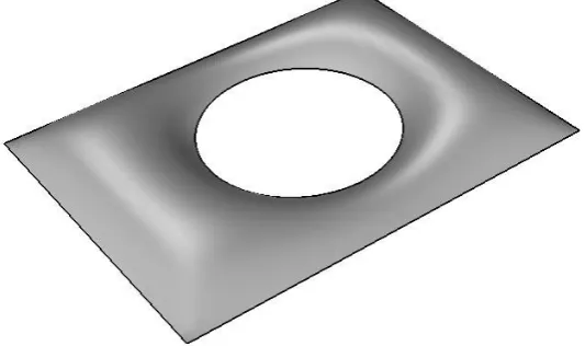
The steel and glass roof of the British Museum Great Court covers a rectangular area 70m wide and 100m long. The Reading Room, which has a cylindrical shape of diameter of 44m, is located near the center of the roof. The shape of the roof was defined by a mathematical function and more information is provided by Williams (2001), with the original trimmed surface shown graphically in Fig. 23.
Fig. 23 Original trimmed surface of British Museum Great Court Roof
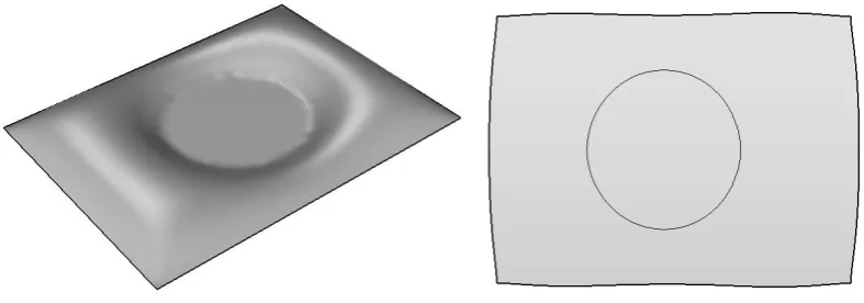
The original surface was obtained analytically (Williams 2001) and a surface reconstruction procedure was
therefore employed to create a NURBS version for this study. The reconstructed NURBS surface was
0 10 20 30 40 50
0 100 200 300 400 500 600 700
varia
nce
of m
em
ber
length
[image:19.595.165.432.531.689.2]discretized and flattened by employing the procedures presented above and the flattened surface is shown in Fig. 24.
Fig. 24 The reconstructed and the flattened surface with trimming boundary
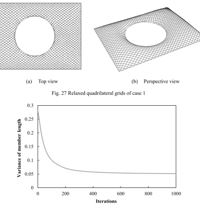
The diagonals were first chosen as the initial guide-lines, as shown in Fig.25. Crossing guide-lines were used to generate the quadrilateral mesh on the flattened surface, and the generated grids were then mapped to the
3D surface. It can be seen from Fig. 26 that the generated grids follow the initial guide-line definition and the grids were generally fluent even without the particle-spring relaxation process being applied. Some very short rods were present close to the boundary, and so vertices very close together at the boundaries were merged.
(a)
(b)
[image:20.595.83.260.627.763.2](a) Top view (b) Perspective view Fig. 26 Quadrilateral grids of case 1
To show the flexibility of the grid generation process, Case 1 above was then relaxed using the particle-spring method and the results are shown in Fig. 27. Compared to the unrelaxed results in Fig. 26, fewer short
rods are observed along their boundary curves. Fig. 28 shows the decreasing variability in member length as more iterations of the grid relaxation method are carried out.
[image:21.595.102.499.242.652.2](a) Top view (b) Perspective view
[image:21.595.137.462.440.649.2]Fig. 27Relaxed quadrilateral grids of case 1
Fig. 28 Change of member length to the iterations for the quadrilateral grid
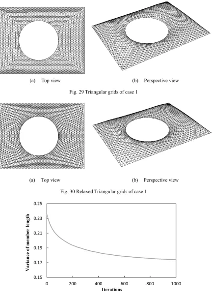
By generating the diagonals of each quadrilateral grid cell, as shown in Fig. 29, a triangular grid was obtained.
Since the new diagonal rods were not very smooth, with kinks especially where they cross the diagonals of the roof, the grid relaxation procedure was further employed on the triangular grid and the results are shown in Fig. 30, leading to more fluent grids and fewer kinks. Fig.31 shows the decreasing variation of member
0 0.05 0.1 0.15 0.2 0.25 0.3
0 200 400 600 800 1000
length with regard to the iterations of grid relaxation.
(a) Top view (b) Perspective view
Fig. 29 Triangular grids of case 1
[image:22.595.86.519.123.734.2](a) Top view (b) Perspective view
[image:22.595.138.456.530.720.2]Fig. 30 Relaxed Triangular grids of case 1
Fig. 31 Variance of member length to the iterations for the triangular grid
0.15 0.17 0.19 0.21 0.23 0.25
0 200 400 600 800 1000
Va
ria
nce of
m
em
ber
length
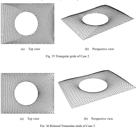
Case study #2 uses two slightly different initial guide-lines, as shown in Fig. 32, with the diagonals curved to cross closer to one of the shorter boundaries of surface. The resulting grid (shown in Fig. 33) is then taken through the same stages of processing as described above, with the relaxed quadrilateral grid shown in Fig. 34, the triangular grids shown in Fig. 35 and the relaxed triangular grids are shown in Fig 36.
Fig. 32 Case 2: initially sketched guide lines on (a) reconstructed complete surface and (b) flattened surface
[image:23.595.77.520.373.816.2](a) Top view (b) Perspective view
Fig. 33 Quadrilateral grids of Case 2
Fig. 34 Relaxed quadrilateral grids of Case 2
(a) Top view (b) Perspective view
Fig. 35 Triangular grids of Case 2
[image:24.595.77.522.89.501.2](a) Top view (b) Perspective view
Fig. 36 Relaxed Triangular grids of Case 2
Fig. 37 Case 3: initially sketched guide lines on (a) reconstructed complete surface and (b) flattened surface
[image:25.595.79.523.281.690.2](a) Top view (b) Perspective view
Fig. 38 Quadrilateral grids of Case 3
(a) Top view (b) Perspective view
[image:25.595.108.513.297.453.2](a) Top view (b) Perspective view Fig. 40 Triangular grids of Case 3
[image:26.595.81.528.67.457.2](a) Top view (b) Perspective view
Fig. 41 Relaxed triangular grids of Case 3
It can be seen from these three case studies that by defining different guide-lines on the surface, various reasonable and smooth options for a gridshell roof can be obtained quickly that respond to the intent of the designer.
A stadium roof
the resulting grids are fluent and the rod lengths near the boundary are changed locally near the boundary curves.
(a) Top view (b) Perspective view
Fig. 42 Trimmed surface
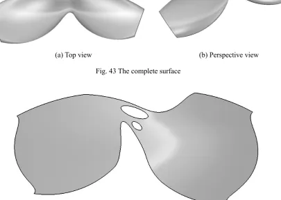
[image:27.595.79.530.126.687.2](a) Top view (b) Perspective view
Fig. 43 The complete surface
[image:27.595.98.504.348.637.2](a) Top view
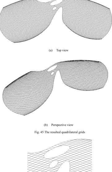
[image:28.595.104.467.93.650.2](b) Perspective view
[image:28.595.193.405.544.658.2]Fig. 45The resulted quadrilateral grids
Trimmed surface with round hole
[image:29.595.126.475.256.400.2]Another roof surface from practice has been used as case of study to underpin the framework proposed. The original surface sketched by the architects is shown in Fig. 47. The entire surface and the boundary curves were flattened using the procedure in Section 3 and the results are presented in Fig. 48. The guide-lines were then advanced on the flattened surface and mapped back to the original surface as shown in Fig. 49 and Fig. 50 using the method described in Section 4 to generate triangular and quadrilateral grids.
[image:29.595.221.373.481.642.2]Fig. 47 Original surface
(a) Top view (b) Perspective view
Fig. 49 The resulted quadrilateral grids
[image:30.595.113.492.85.237.2](a) Top view (b) Perspective view
Fig. 50 The resulted triangular grids
It is worth noting that the initial guide lines defined over the surface set the tone of the grid and reveal
the intent of the designer. What kind of initially defined guide lines are the more favourable pattern in
terms of appearance most likely depends on the individual preference of the architect.
length and merging several curve segments into a single curve for further operations. The software is also able to exchange data with other commercial software packages as part of an integrated design process using data formats such as IGES, STEP, BREP, and STL.
Conclusions
A grid generation and relaxation technique for free-form surfaces with complex boundaries is proposed for the design of structural gridshells, based on a surface flattening technique and an improved guide-line method. The parametric domain of the complete NURBS surface is firstly divided into a number of parts and a discrete free-form surface is formed by mapping dividing points onto surface. The free-form surface is then flattened based on the principle of identical area. Accordingly, a flattened rectangular lattice is generated on the 2D surface by employing the guide-line method and complex boundaries are dealt with by removing segments of the curves outside the design domain. The 2D grids are then mapped back onto the 3D surface, and a mass-spring method employed to further improve the smoothness of the resulting grid.
The results not only meet the requirements of regular shapes and fluent lines, but they also embody the design intent of the grids and have a high quality around the inner boundary.
The proposed framework can efficiently generate grids for design of free-form gridshell with both internal and external boundaries and the framework has been shown to be useful in facilitating the conceptual design process of free-form gridshells in engineering practice.
Acknowledgements
This research was sponsored by the National Natural Science Foundation of China under Grant 51378457, Grant 51678521 and Grant 51778558 and by the Natural Science Foundation of Zhejiang Province under Grant LY15E080017. This financial support is gratefully acknowledged by the authors.
References
Adriaenssens, S., L. Ney, E. Bodarwe and C. Williams (2012). "Finding the form of an irregular meshed steel and glass shell based on construction constraints." Journal of Architectural Engineering 18(3): 206-213.
Aubry, R., G. Houzeaux and M. Vazquez (2011). "A surface remeshing approach." International Journal for Numerical Methods in Engineering 85(12): 1475-1498.
Banchoff, T. F. and S. T. Lovett (2015). Differential geometry of curves and surfaces, CRC Press.
Barnes, M. (1977). Form finding and analysis of tension space structures by dynamic relaxation, PhD thesis, City University London.
Douthe, C., R. Mesnil, H. Orts and O. Baverel (2017). "Isoradial meshes: Covering elastic gridshells with planar facets." Automation in Construction 83: 222-236.
Gao, B., C. Hao, T. Li and J. Ye (2017a). "Grid generation on free-form surface using guide line advancing and surface flattening method." Advances in Engineering Software 110: 98-109.
Gao, B., T. Li, T. Ma, J. Ye, J. Becque and I. Hajirasouliha (2017b). "A practical grid generation procedure for the design of free-form structures." Computers & Structures 196:292-310
Hannaby, S. A. (1988). "A mapping method for mesh generation." Computers & Mathematics with Applications 16(9): 727-735.
Kang, W., Z. Chen, H.-F. Lam and C. Zuo (2003). "Analysis and design of the general and outmost-ring stiffened suspen-dome structures." Engineering Structures 25(13): 1685-1695.
Kilian, A. and J. Ochsendorf (2005). "Particle-spring systems for structural form finding." Journal of the International Association for Shell and Spatial Structures 148(77): 30-38.
Lefevre, B., C. Douthe and O. Baverel (2015). "Buckling of elastic gridshells." Journal of the International Association for Shell and Spatial Structures 56(3):153-171
Li, J., D. Zhang, G. Lu, Y. Peng, X. Wen and Y. Sakaguti (2005). "Flattening triangulated surfaces using a mass-spring model." The International Journal of Advanced Manufacturing Technology 25(1-2): 108-117.
Liu, Y., H. L. Xing and Z. Q. Guan (2011). "An indirect approach for automatic generation of quadrilateral meshes with arbitrary line constraints." International Journal for Numerical Methods in Engineering 87(9): 906-922. Malek, S. and C. J. Williams (2017). "Reflections on the Structure, Mathematics and Aesthetics of Shell Structures." Nexus Network Journal 19(3): 555-563.
McCartney, J., B. Hinds and K. Chong (2005). "Pattern flattening for orthotropic materials." Computer-Aided Design 37(6): 631-644.
Muylle, J., P. Iványi and B. Topping (2002). "A new point creation scheme for uniform Delaunay triangulation." Engineering Computations 19(6): 707-735.
Piegl, L. and W. Tiller (2012). The NURBS book, Springer Science & Business Media.
Popov, E. V. (2002). Geometric approach to chebyshev net generation along an arbitrary surface represented by NURBS. International Conference on Computer Graphics and Vision, 2002.
Richardson, J. N., S. Adriaenssens, R. F. Coelho and P. Bouillard (2013). "Coupled form-finding and grid optimization approach for single layer grid shells." Engineering Structures 52: 230-239.
Shepherd, P. and P. Richens (2012). "The case for subdivision surfaces in building design." Journal of the International Association for Shell and Spatial Structures 53(4): 237-245.
Shilin, D. (2010). "Development and expectation of spatial structures in China." Journal of Building Structures 6: 006.
Su, L., S. L. Zhu, N. Xiao and B. Q. Gao (2014). "An automatic grid generation approach over free-form surface for architectural design." Journal of Central South University 21(6): 2444-2453.
Topping, B. and A. Khan (1994). "Parallel computation schemes for dynamic relaxation." Engineering Computations 11(6): 513-548.
Topping, B. H. and P. Iványi (2008). Computer aided design of cable membrane structures, Saxe-Coburg Publications.
Wang, C. C. and K. Tang (2007). "Woven model based geometric design of elastic medical braces." Computer-Aided Design 39(1): 69-79.
Williams, C. J. (2001). "The analytic and numerical definition of the geometry of the British Museum Great Court Roof." In: Mathematics & design 2001; Deakin University, 434-440.
for computer-aided engineering." Computer Physics Communications 190: 1-14.