The demand for food in south Africa 1

(1)

The Demand for Food in South Africa

Paul Dunne

University of the West of England, Bristol and SALDRU, University of Cape Town

and

Beverly Edkins

University of KwaZulu-Natal

August 2005

Abstract

Food consumption is an important issue in South Africa, not only in its relation to poverty and deprivation, but also given the importance of nutrition in allowing HIV/AIDS sufferers to lead extended, productive lives. With the pressing need to increase food security and the enormity of the epidemic, understanding the demand for food has become a vital task. It is important that the determinants of the demand for food are understood, so that responses of household food consumption to changes in the prices of foodstuffs, prices of other commodities, and total expenditure can be anticipated. There is, however, surprisingly little economic research on this topic. This paper provides an empirical analysis of the demand for food in South Africa for the years 1970 to 2002. It uses two modelling approaches, a general dynamic log-linear demand equation and a dynamic version of the almost ideal demand system to provide estimates of the short- and long-run price and expenditure demand elasticities.

Paper presented to Economics Society South Africa Conference, Durban, September, 2005. we are grateful to participants, Lawrence Edwards, Peter Howells and Ron Smith for comments. Correspondence to: John2.Dunne@uwe.ac.uk

(2)

1. INTRODUCTION

Studies of food consumption and expenditure have often been the subject of research in the developed and developing world. They provide important inputs into food and related nutritional policy initiatives, by providing estimates of how food consumption is likely to change with changes in prices, incomes and taxation. In the context of South Africa food policy is inextricably linked to food security. Despite its status as a

lower-middle-income-country (World Bank website), it has considerable inequality and deprivation. It is estimated that about 35 per cent of the population in South Africa are vulnerable to food insecurity and approximately a quarter of the children under the age of 6 years are estimated to have had their growth stunted by malnutrition (Human Sciences Research Council, 2004, 3). Thus, the Department of Agriculture devised ‘An Integrated Food Security Strategy for South Africa’ (IFSS) in July 2002. Food also has special significance, in the fight against HIV/AIDS. Nutrition is known to be important in determining the body’s ability to cope with HIV/AIDS and a well nourished body is essential for ensuring those living with the disease lead extended, productive lives. This means that it is important to be able to anticipate the types of changes that can take place in the food consumption of households when there are changes in incomes, prices and taxation.

Understanding the demand for food is, therefore, a vital task, but there is, however, surprisingly little economic research on this topic. The main recent studies are

(3)

estimation, others using systems of equations, some sticking with static models and others introducing dynamic models in a number of ways. Add to this the different definitions in the data and the different samples and it is no surprise that they get a range of results.

In this paper a time series analysis of the demand for food in South Africa for 1970 – 2002 is undertaken. Rather than focus on one particular method it takes both an ‘ad hoc’ approach, estimating a general dynamic log-linear demand equation, as well as a ‘demand system’ approach, estimating a dynamic form of the almost ideal demand system (Deaton and Muellbauer, 1980). These provide estimates of price and income elasticities in both the short run and the long run. In the next section a brief description of food and related data trends in South Africa is provided, followed in section 3 by a brief review of demand theory and the econometric approaches used in empirical work. Sections 4 and 5 then consider the South African data, discussing the empirical models and the result of estimating them on the South African data. The elasticity estimates are summarised and discussed in section 6. Finally, section 7 presents some conclusions and considers how the work could be developed in future.

2. Food and related data trends in South Africa

The main source of consistent time series data on food and other consumption is the Reserve Bank of South Africa web site, ‘Quarterly Bulletin Time Series”. Under this data the category for ‘food’ is classified as ‘food, beverages and tobacco’. The variables include expenditure on food (in constant prices) (Qt), total consumers’ expenditure in

current prices (Xt), the price of food (PFt), and a general price index (PGt).

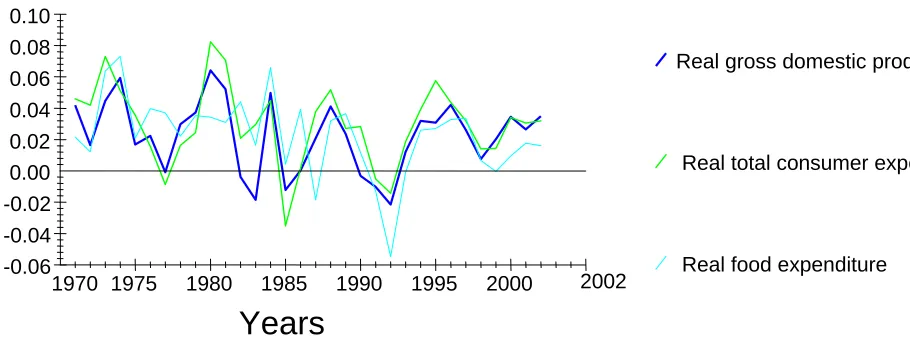
Figure 1 shows the growth of real food expenditure, real total consumer expenditure and real gross domestic product (GDP)1. This shows the period under consideration,

1

(4)

[image:4.612.106.561.334.509.2]

2002 to be one of poor growth in GDP. In the 1960s the real average annual growth was 5.8 % (Akinboade et al., 2004), slowing to 3.31% in the 1970s and 1.50% per annum in the 1980s. Growth then improved in the 1990s to average 1.73% per annum and 3.5% in 2002. As expected, the growth of consumer expenditure followed a similar pattern to the growth of real GDP, averaging 3.78% per annum in the 1970s, 2.77% per annum in the 1980s and 2.34% per annum for the 1990s. Between 2001 and 2002 total consumption expenditure grew at 3.19 %.

Figure 1: Growth rates of real gross domestic product, food expenditure and total consumer expenditure

While food expenditure followed a similar pattern, the deterioration of growth was more marked, with average growth in the 1970s at 3.59% per annum, declining to 2.62% per annum in the 1980s and a meagre 0.66% per annum for the 1990s. 2001-2 saw growth of 1.61%.

Real gross domestic product

Real total consumer expenditure

Real food expenditure

Years

-0.02 -0.04 -0.06 0.00 0.02 0.04 0.06 0.08 0.10

(5)

As Table 1 shows, the share of food in expenditure also fell over this period2. In 1970 the share of consumer expenditure devoted to food was 35.6%, by 1990 it was 34.5%,

declining markedly in the 1990s, to reach 28.4% in 2002. The categories that showed increases in their share were transport, housing, clothing and medical services, with expenditure on furniture showing a small decline over the period.

Table 1: Budget shares (percentages) of consumer spending, South Africa, 1970 – 2002

Year Food Transport Housing Furniture Clothing Medical Recreation

All other goods and services

1970 35.63 16.81 6.54 11.46 5.84 3.48 7.40 12.84

1975 33.67 16.25 5.70 12.42 6.22 4.30 8.26 13.18

1980 34.98 16.61 7.28 12.40 6.08 4.29 8.11 10.25

1985 36.08 13.42 11.10 11.61 5.18 4.69 7.75 10.17

1990 34.47 15.56 11.47 11.04 5.08 4.86 6.87 10.65

1995 30.81 17.41 11.80 10.80 6.13 6.35 6.80 9.90

2000 29.14 17.97 11.04 10.25 6.35 6.43 7.39 11.43

2002 28.38 18.77 10.67 10.07 7.21 6.76 7.70 10.44

Mean 33.43 16.17 9.51 11.43 5.90 4.96 7.42 11.18

3. Analysing the Demand for Food

To analyse the demand for food a useful starting point is the neoclassical model of consumer choice. This suggests the demand is the outcome of a consumer making a utility-maximising decision, based on the prices of all products available to the consumer, and the consumer’s total expenditure. Thus the demand function is specified as

2

(6)

qi = qi(p1, p2, ..., pn, x) i = 1, 2, …, n. (1)

where qi and piare the quantity demanded and price of the ith product, there are n

products in total, and x =

∑

p

i iqi is total expenditure. Empirical studies of demand

using econometrics have used single demand equations of particular commodity groups and systems of demand equations.

For single equation models the theory provides limited information. It does not specify the precise form of the equation, nor variables to be included, other than prices and income. It does, however, suggest certain restrictions which can help limit the degrees of freedom lost. Demand functions are considered homogenous of degree zero in all

explanatory variables and the Slutsky conditions imply that own-price substitution effects are negative and the own-price and income derivatives of a demand equation should be δqi/δpi + qi(δqi/δx) < 0.

As theory does not provide much in the way of guidelines for the specification of a demand equation, empirical versions of demand equations are often relatively ad hoc. Functional forms are chosen to facilitate easy estimation, and explanatory price variables usually include own-price, the price of close substitutes and complements and possibly the general price level. Specifications in logarithms have the advantage that the

coefficients estimated can be interpreted as elasticities. This general specification is followed for our food demand equation.

qi = β0 + β1pi + β2 pj + β3 pg + β4x + u (2)

Where qiis the quantity demanded of good i, piis the price of good i, pjis the price of

good j, pg is the general price level, and x is current total expenditure. To allow for dynamic analysis, lags of the dependent variable and explanatory variables are introduced.

(7)

freedom to be increased through single equation and cross equation restrictions3. The most popular system in the literature, due to its flexibility and ease of use is the almost ideal demand system of Deaton and Muellbauer (1980):

wi = αi + Σk δk Dk + Σj γij ln pj + βi ln (E/P) (3)

where lnP = α0 + Σk αk ln pk + ½ Σj Σk γkj ln pj ln pj,E is total expenditure, wi = pi qi / E

and the conditioning variables Dk can determine the intercepts of the demand functions.

The system can be estimated equation by equation by using the approximation for lnP, ln

P* = Σj wj ln pj. This is a static model but has been made dynamic in the literature by

respecifying the theory (Dunne et al., 1984), or by specifying a general dynamic

estimable form of the regression (Anderson and Blundell, 1987; Smith, 1989). The latter approach is used below.

Given the importance of the issue for South Africa, there has been surprisingly little research on the demand for food. In a recent contribution Taljaard et al. (2004) focus on the demand for meat, using an almost ideal demand system, while Selvanathan and Selvanathan (2003) estimate a version of the Rotterdam demand system for a range of groups of commodities, but they do not focus particularly on food and give it little attention. Agbola et al. (2003) examine cross-sectional data from the South African Integrated Household Survey (SAIHS) of 19934, analysing household consumption of food groups and estimating price and expenditure elasticities of demand for the food groups. There has also been some research conducted by the Integrated Rural and

Regional Development research programme of the Human Sciences Research Council. It

3

In estimating systems of demand equations, two approaches are used. Firstly, the precise form of the utility function is specified as in the case of the linear expenditure system. Using this approach implies that the system of demand equations derived will satisfy at least some of the general restrictions of consumer theory. The advantage of this approach is that degrees of freedom are saved, but the disadvantages are that the restrictions cannot be tested and there is a loss of generality in specifying the form of the utility

function. The second approach begins with a set of demand equations which possibly satisfy the theoretical restrictions. The advantage of this is that the restrictions can then tested, but at the cost of limiting the degrees of freedom. This is the case for the Rotterdam and almost ideal demand systems.

4

(8)

conducted a pilot study for the Department of Agriculture ‘… to establish a methodology for monitoring and evaluating the impact of … price increases on low-income

communities in both rural and urban areas.’ (Human Sciences Research Council, 2004, 59). The results of this study were presented in 2002 (Aliber and Modiselle, 2002), but the sample size and budget were limited, so the survey only provides useful insight into the impact of price increases on low-income households, and nothing more. HSRC(2004) noted that the survey indicates that during the 6 months April – October 2001, the price of maize meal rose by between 25% and 35%, the sugar price increased by about 20% and the rice price by between 25% and 65%, while average spending on all of the items increased by 28% - the closest to an elasticity measure they get5. Balyamujura et al. (2000) replicated some earlier studies in order to project impact of HIV/AIDS on the demand for food.

Recent international studies of the demand for food include a field trail experiment in applied econometrics reported in Magnus and Morgan (1999) which collected budget survey and time-series for the USA and the Netherlands. Various groups of researchers examined the data using differing techniques and methodologies, including Song, Liu and Romilly (1997). They use an error correction model and an almost ideal demand system, to obtain elasticities.

Recent food related studies using the almost ideal demand system are Eakins and

Gallagher (2003) on alcohol expenditure in Ireland, Duffy (2001) on food demand in the UK, Karagiannis et al. (2000) on the demand for meat in Greece. In the context of major transformation of the US farm and food policy, LaFrance (1999a, 1999b) and LaFrance and Beatty (2001) analysed the demand for food in the US, while Edgerton et al. (1996) estimate demand systems for food for the Nordic countries.

4. Estimating the Demand Equation

5

(9)

To operationalise equation (2) for a time series study a dynamic model is required. Using a general first order log-linear demand model (ARDL) gives:

qt = b0 + b2 qt-1 + b3 pft + b4 pft-1 + b5 pgt + b6 pgt-1 + b7 x t + b8 x t-1 + εt (4)

Reparameterising to provide a specification that allows for easy identification of the long-run effects gives:

∆qt = b0 +b3∆pft + b5∆ pgt + b7∆ x t - α0 qt-1 +α1 pft-1+α2 pgt-1 +α3 x t-1 + εt (5)

Estimating this model for the period 1970-2002 gives the results in Table 2. There are four significant explanatory variable∆pft, ∆ x t, x t-1 and qt-1, with the change in the

general price index, ∆ pgt, the lagged food price, pft-1, and lagged general price, pgt-1

[image:9.612.205.405.377.602.2]

insignificant

Table 2: The dynamic demand model

Variable Coefficient t-ratio (probability)

Constant -1.59 -1.53 (0.14)

∆pft -0.44 -2.75 (0.01)

∆pgt -0.00 -0.00 (0.99)

∆xt 0.54 3.94 (0.00)

qt-1 -0.31 -2.24 (0.04)

pft-1 -0.28 -1.42 (0.17)

pgt-1 -0.16 -1.03 (0.31)

xt-1 0.41 3.22 (0.00)

Diagnostic Test Result (probability)

Standard error 0.02

R2 0.65

Serial Correlation F(1,23) = 0.00 (0.99) Functional form F(1,23) = 1.89 (0.18) Heteroscedasticity F(1,30) = 0.01 (0.93)

Normality Chsq(2) = 0.93 (0.63) Chow test F(8,16) = 0.92 (0.53)

(10)

The restrictions of short-run and long-run homogeneity, imply that the short-run elasticities sum to zero and long-run elasticities sum to zero. This is imposed by introducing the relative price of food and real total consumer expenditure into the

equation in place of the price of food and current total consumer expenditure. This gives:

∆qt =ρ2∆rpft +ρ3∆r x t - ρ1(qt-1 - ρ0 - ρ4r pft-1 - ρ 5 rx t-1)+ vt (6)

or

∆qt = τ0 - ρ1qt-1 + ρ2∆rpft +ρ3∆rx t + τ1rpft-1 + τ 2 rx t-1 (7)

Where τ0 = ρ0 ρ1, τ1= ρ1ρ4 , and τ 2 = ρ1ρ5

[image:10.612.173.439.392.592.2]

As the results in Table 3 show, all five explanatory variables are significant when these restrictions are imposed. The only diagnostic test to suggest a problem is that for the functional form. The F-test for the homogeneity restrictions indicate that they are not rejected.

Table 3: The dynamic demand model with homogeneity imposed

Constant -0.14 -0.41 (0.69)

∆rpft -0.55 -3.39 (0.00)

∆rxt 0.49 3.48 (0.00)

qt-1 -0.31 -2.66 (0.01)

rpft-1 -0.39 -2.02 (0.05)

rxt-1 0.29 2.40 (0.02)

Diagnostic test Result (probability)

Standard error 0.02

R2 0.57

Normality Chsq(2) = 0.71 (0.69) Homogeneity restrictions F(2,24) = 2.65 (F0.05(2,24) = 3.40)

(11)

by severe cold spells in winter combined with drought conditions in summer (South African Reserve Bank Quarterly Bulletin,March 1973). Secondly, Rutter (2003) studying the determinants of the South African producer price of maize from 1970 to 2001 also observed an outlier for 1972, which he suspected was due to a deal between the US and Russia on the sale of wheat, which had a knock on effect on feed grain prices (Lutterell, 1973) and so the South African grain industry. Thirdly, the Foodstuffs, Cosmetics and Disinfectants (FCD) Act came into being in 1972 (Act 54 of 1972). It falls within the ambit of the government’s Health Department, but covers all foodstuffs sold in South Africa (The South African Market for Food and Beverages Report, 1997).

[image:11.612.176.440.404.608.2]

Introducing a dummy variable for 1972 to the error correction model with homogeneity imposed gives the results in Table 4. The dummy is significant and its inclusion deals with the functional form issue and the homogeneity restrictions are still not rejected6. .

Table 4: The dynamic demand model with homogeneity imposed and a 1972 dummy

Constant -0.05 -0.17 (0.87)

∆rpft -0.60 -4.15 (0.002)

∆rxt 0.50 3.98 (0.00)

qt-1 -0.37 -3.56 (0.00)

rpft-1 -0.46 -2.63 (0.01)

rxt-1 0.35 3.15 (0.00)

D72 -0.05 -2.92 (0.01)

Diagnostic Test Result (probability)

Standard error 0.02

R2 0.68

6

(12)

This means that the short-run elasticities of demand with respect to the relative price of food and real total consumer expenditure are -0.6 and 0.5 respectively, while the values of the coefficients on the lagged levels suggest a long-run relation:

q= -1.24rpf + 0.95rx

Thus the long-run elasticities are -1.2 with respect to the relative price of food and 0.95 with respect to real total consumer expenditure. Testing for unitary elasticities by imposing them on the equation, saw the price elasticity restriction rejected, but the income elasticity is not rejected7.

These results suggest that the demand for food is more responsive to price and income changes in the long run than in the short run. This would be expected for food as short-run consumption behaviour is likely to be affected by habit and other factors, whereas in the long run consumers have time to adjust. The fact that the long-run income elasticity result is nearly unity could be the result of the high proportion of poor households in the South African population. As incomes rise it is largely matched by rising expenditure on food in the long run.

The long-run price elasticity of -1.2 is a concern, as it is much larger than one might expect for a necessity. This might result from the definition of food in the data. In fact the category is ‘food, beverages and tobacco’. While this is in common use, it could be argued that the constituent components act differently. Thus, when there is an own-price increase, the consumption of tobacco and alcoholic beverages may be reduced fairly substantially to ensure basic food needs are met. On the other hand the addictive nature of these goods might limit such adjustments in practise.

7

The joint restriction that the coefficients on rpf and rx were 1 and -1 respectively, in equation 6 with D72 included, was rejected: F(2,25) = 5.73 and F0.05(2,23) = 3.39. Likewise, testing the coefficient on rpf was 1

was rejected: F(1,25) = 9.67 and F0.05(1,25) = 4.24. However, the restriction that the coefficient on rx was

(13)

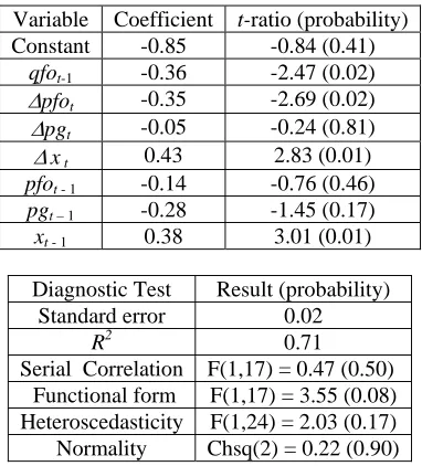
It is possible to get a variable with a less broad definition of food from the South African Reserve Bank, but only for the shorter period 1976-2003. Using this ‘only food’ variable in equation (5)gives:

∆qfot =θ0 + θ1 qfot-1+ θ2∆pfot + θ3∆ pgt + θ4∆ x t + θ5pfot - 1

+ θ6 pgt -1+ θ7 x t -1 +υt (8)

where qfotis consumer expenditure on ‘only food’ and pfot is the price of ‘only food’, and

[image:13.612.211.402.337.548.2]

other variables are as previously defined. The results suggest a relatively well specified model, for which the homogeneity restriction is not rejected8.

Table 5: The dynamic demand model: ‘only food’

Variable Coefficient t-ratio (probability) Constant -0.85 -0.84 (0.41)

qfot-1 -0.36 -2.47 (0.02)

∆pfot -0.35 -2.69 (0.02)

∆pgt -0.05 -0.24 (0.81)

∆x t 0.43 2.83 (0.01)

pfot - 1 -0.14 -0.76 (0.46)

pgt – 1 -0.28 -1.45 (0.17)

xt - 1 0.38 3.01 (0.01)

Diagnostic Test Result (probability) Standard error 0.02

R2 0.71

Normality Chsq(2) = 0.22 (0.90)

Imposing the homogeneity restriction gives the results in Table 6, with all the explanatory variables significant, except for rpfo t -1, the lagged relative/real price of food, and no

obvious specification problems.

8

The relevant equation to test homogeneity is:

∆qfot =γ 0 + γ 1 qfot-1+ γ 2∆rpfot + γ 3 ∆rx t + γ 4rpfot - 1 + γ 5 rx t -1 + ut

(14)

With the more restricted definition of food, the elasticities are indeed lower, with the short-run price elasticity -0.5 and the income/expenditure elasticity is 0.5. The long-run relationship is:

qfo= -0.77rpfo + 0.63rx

[image:14.612.193.423.339.535.2]

This implies a long-run price elasticity of -0.8, though this is based on an insignificant coefficient for the relative price and an expenditure elasticity of 0.6. That the long-run relative price term should be insignificant is not unexpected. As Thomas (1997) argues in a study of food demand in the USA, food is a very basic necessity and it would be reasonable to assume that the demand for it may well be eventually unaffected by its price and only be determined by real income/expenditure9.

Table 6: The dynamic demand model with homogeneity imposed: only food

Variable Coefficient t-ratio (probability)

Constant 1.03 1.93 (0.07)

qfot-1 -0.35 -3.16 (0.01)

∆rpfot -0.48 -3.63 (0.00)

∆rxt 0.45 2.73 (0.01)

rpfot -1 -0.27 -1.45 (0.16)

rxt -1 0.22 2.52 (0.02)

Diagnostic Test Result (probability)

Standard error 0.02

R2 0.63

Serial Correlation F(1,19) = 0.04 (0.84) Functional form F(1,19) = 2.13 (0.16) Heteroscedasticity F(1,24) = 3.62 (0.07) Normality Chsq(2) = 0.03 (0.98) Restrictions F(2,18) = 2.56 F0.05(2,18) = 3.55

These results do seem to support our concern with the composition of the food category, excluding beverages and tobacco from the data reduces the elasticities and suggests that own price is not an important variable in the long-run, but moving to the ‘food only’ category is at the cost of degrees of freedom. The income elasticity estimates show food

9

(15)

to be a normal good, its demand increases as income increases, and it is inelastic in both the short-run and long-run. Again this meets expectations for a necessity.

5. Estimating a Demand System

In using the ‘demand system’ approach, the almost ideal demand system of equation (3) is employed in a dynamic form, following Smith (1989). The system has two equations; one for food and a residual category non-food:

∆sqt = λ10+ λ11∆pft + λ12∆ pnft + λ13∆( x - P*)t - λ14 sqt-1 + λ15 pft-1

+ λ16 pnft-1 + λ17( x - P*) t-1+ ε1 (8)

∆snfqt = λ20+ λ21∆pft + λ22∆ pnft + λ23∆( x - P*)t - λ24 sqt-1 + λ25 pft-1

+ λ26 pnft-1 + λ27( x - P*) t-1+ ε2 (9)

Where, sqt is the share of expenditure on food and snfqt, the share of non-food

expenditure, pft the price of food, pnft the non-food price and (x - P*) is the log of

[image:15.612.191.412.485.681.2]

consumption expenditure in current prices minus the log of an index of prices, P*10.Note that the dependent variable no longer sums to one, the dynamic form it is not a singular system. The estimation results for the food equation are given in Table 8.

Table 8: Dynamic almost ideal demand system

Variable Coefficient t-ratio (probability)

Constant -0.24 -0.62 (0.54)

∆pft -0.1 -2.23 (0.04)

∆pnft 0.14 2.6 (0.02)

∆ (x – P*)t -0.16 -3.39 (0.00)

sqt-1 -0.35 -2.56 (0.02)

pft-1 -0.06 -1.41 (0.17)

pnft-1 0.06 1.20 (0.24)

( x – P*) t-1 0.03 0.94 (0.36)

Measure/ Diagnostic Test Result (probability)

Standard error 0.01

R2 0.68

Serial Correlation F(1,23) = 0.01 (0.93) Functional form F(1,23) = 0.05 (0.83)

10

(16)

Heteroscedasticity F(1,30) = 0.92 (0.35) Normality Chsq(2) = 0.95 (0.62)

All the coefficients on the changes variables are significant, as is the lagged dependent variable sqt-1. However, the three long-run coefficients are all insignificant. The results

for the diagnostic tests suggest no particular problems with the specification of the model.

Imposing homogeneity on the system implies using the relative price of food, so taking

pff

∆ t = ∆pft - ∆ pnft and pfft-1 = pft-1 - pnft-1 gives for food:

∆sqt = δ10 +δ 11∆pfft + δ 12∆( x - P*)t + δ 13 sqt-1 +δ 14 pfft-1

+δ 15( x - P*) t-1+ υ1 (10)

[image:16.612.169.444.379.577.2]

Estimating equation (10) gives the results in Table 9.

Table 9: Dynamic almost ideal demand system with homogeneity imposed:

Constant 0.17 1.74 (0.09)

∆pfft -0.14 -3.73 (0.00)

∆ (x – P*)t -0.17 -3.52 (0.00)

sqt-1 -0.34 -2.78 (0.01)

pfft-1 -0.09 -2.04 (0.05)

( x – P*) t-1 -0.01 -0.67 (0.51)

Standard error 0.01

R2 0.61

Homogeneity is not rejected and the only insignificant explanatory variable is ( x - P*) t-1,

though the significance of the relative price, pfft-1, coefficient is borderline. The four tests

(17)

Within the demand system the coefficients are not elasticities, they are measuring the response of shares to changes in price and income, though a negative sign on the income/expenditure coefficient does indicate that food is an inferior good.

For the long-run (static) model:

sqt = κ10+κ11pfft + κ12 ( x - P*)t (16)

the expenditure elasticity is: ef = 1 +

t

sq

12

κ

meaning that if κ₁₂ is not significantly different to zero, there is a unit income elasticity. The compensated own price elasticity of for food is:

pef =

[

(

x P

)

]

sq

sq + − * −1+

1

23 12

11 κ κ

κ

and the uncompensated is pef – ef sq. For the short-run elasticities we replace the long-run

coefficients with the short-run ones. Computing the short-run elasticities gives a value of 0.5 for income elasticity and 0.0 for the compensated price elasticity, with the latter being rather different to that calculated using the log-linear model. The long-run elasticities are 1 for income (as expected given the insignificance of the total real expenditure term) and -0.9 for price.

[image:17.612.196.417.616.707.2]

Estimating the model for 'only food' gives the results in Table 10, which shows insignificant coefficients on the change of real total expenditure change and its lagged level, but with no obvious specification problems.

Table 10: Dynamic almost ideal demand system for ‘only food’

Constant 0.13 0.42 (0.68)

∆pfot -0.11 -3.33 (0.00)

∆pnfot 0.16 3.11 (0.01)

∆ (x – PO*)t -0.06 -0.79 (0.44)

sqot-1 -0.60 -3.44 (0.00)

(18)

pnfot-1 0.01 2.16 (0.05)

( x – PO*) t-1 0.00 0.00 (0.10)

Standard error 0.00

R2 0.69

Normality Chsq(2) = 1.27 (0.53)

[image:18.612.195.417.73.198.2]

Imposing homogeneity gives the results in Table 11 and the restriction is not rejected. It shows the coefficients on the real expenditure terms to be insignificant, though the lagged level is significant at 6%, suggesting that the calculated short-run income elasticity of demand is one. All the other regressors are significant and there are no obvious problems with the specification.

Table 11: Dynamic almost ideal demand system for ‘only food’ with homogeneity imposed:

Constant 0.23 2.78 (0.01)

∆pffot -0.12 -4.11 (0.00)

∆ (x – PO*)t -0.03 -0.50 (0.62)

sqot-1 -0.52 -3.95 (0.00)

pffot-1 -0.12 -3.29 (0.00)

( x – PO*) t-1 -0.01 -1.98 (0.06))

Standard error 0.00

R2 0.68

(19)

[image:19.612.101.507.379.418.2]

6. The Demand for Food

Table 12 presents the elasticity estimates found in the empirical analysis above. Looking at food, tobacco and alcohol results the two methods give similar estimates for the income elasticities 0.5 for the short run and 1 for the long run. They differ in their price elasticity estimates, though both show lower short-run than long-run values. The demand system gives smaller price elasticities, in the short-run it is equal to zero, the long-run elasticities are closer, with the demand equation just over one and the demand system just under one. Using food only, at the cost of degrees of freedom, gives smaller long-run elasticities for the demand equation as we were expecting, but not for the system.

Table 12: Elasticity Estimates

Demand equation: Food, tobacco, alcohol

Time period Price elasticity of demand Uncompensated Income elasticity of demand

Short-run -0.6 -0.5 0.5

Long-run -1.2 -1.6 0.9

Demand equation: Food only

Short-run -0.5 -0.4 0.5

Long-run -0.8 -0.9 0.6

Demand system: Food, tobacco, alcohol

Short-run -0.0 -0.2 0.5

Long-run -0.9 -1.3 1.0

Demand system: Food only

Short-run -1.2 -1.4 0.9

Long-run -1.3 -1.5 1.0

[image:19.612.101.506.594.634.2]

(20)

elastic (although the estimate is -0.9 for the system) suggesting that an increase in price will lead to a more than proportionate decline in demand. Food, the more restrictive category, is price inelastic, though close to one for the demand equation, but price elastic for the system. Food, alcohol and tobacco seem to have unit income elasticity, implying that it will increase proportionately with income. Food alone, again produces different results for the equation, it is income inelastic, and for the system, the income elasticity is unity.

The short-run elasticity estimates are also not completely consistent across the two estimation approaches, but they are generally smaller than the long-run elasticities. Food, alcohol and tobacco would seem to be price and income inelastic, while food alone, is the same for the demand equation, but is price elastic for the system, with almost unit

elasticity.

[image:20.612.304.499.507.652.2]

Considering other recent estimates, the Selvanathan and Selvanathan (2003) consumer demand system study, 19602001, gives an estimate for the price elasticity of food of -0.32 and for income elasticity of food is 0.81. Balyamujura et al. (2000), using a single equation model of demand described earlier in the paper, estimate that the price elasticity of demand, in terms of the consumer price index, is -0.90 and the income elasticity of the demand for food is 0.58. Other earlier studies found somewhat lower estimates.

Table 13: A summary of earlier studies on elasticity estimates

Period Price Income

Elasticity Elasticity

Dockel and Groenwald (1970) 1947-68 -0.3 0.6

Barr (1983) 1946-73 SR -0.4 SR 0.95 LR -0.2 LR 0.62 Contigiannis (1982) 1960-79 SR -0.2 SR 0.2

LR -0.1 LR 1.4 Selvanathan and Selvanathan (2003) 1960-2001 -0.3 0.8 Balyamujura et al. (2000) 1970- 1998 -0.9 0.6

(21)

higher elasticities (larger negative in the case of prices), but our results are suggesting values beyond the other studies. This illustrates the importance of recognising the need to compare the results of different empirical methods and to be careful of taking the results of any particular empirical analysis as the basis for policy.

7. CONCLUSION

This paper has provided an empirical analysis of the demand for food in South Africa for the period 1970 – 2003. Rather than focussing on one particular method it has taken an ‘ad hoc’ approach, estimating a general dynamic log-linear demand equation, as well as a ‘demand system’ approach, estimating a dynamic form of the almost ideal demand system (Deaton and Muellbauer, 1980). These have both provided estimates of long-run and short-run price and income elasticities, but they were not wholly consistent. Further concerns with the definition of food led to estimates being made for food, alcohol and tobacco and for a more restrictive definition of food, though this was at the expense of degrees of freedom.

The empirical analysis has allowed us to make some tentative conclusions, but possibly more importantly provides an important warning of the need to consider a range of approaches and studies if feeding the results into policy recommendations. Previous studies have often started from similar theoretical background, but differ markedly in the way they operationalise their models, some using single equation estimation, others using systems of equations, some sticking with static models and others introducing dynamic models in a number of ways. Together with possible different definitions of the data and lengths of time series, it is not surprising that there can be a range of results.

(22)

to have unit income elasticity, implying that it will increase proportionately with income. Food, the more restrictive category, is less elastic, but the results suggest unit elasticity or higher. For income it is either inelastic or unit elasticity.

The short-run elasticity estimates were not completely consistent across the two

estimation approaches, but they were generally smaller than the long run. Food, alcohol and tobacco would seem to be price and income inelastic, while for food the result veers between price inelastic and price elastic, with almost unit income elasticity. Comparing these results with earlier studies the elasticities are considerably higher.

Information on elasticity estimates can provide policy makers with an indication of how South African consumers react to changes in the price of food, taxes and changes in income. Such changes may arise directly through food and nutrition polices, or from adjustments within the economy, whether it is the growth of the economy or, for example, some adverse shock to the agriculture sector. With a knowledge of price and expenditure elasticities, policies which aim to alleviate food insecurity and have a positive impact on nutrition, and reduce the impact of HIV/AIDS impact, can be more readily assessed11. The size of the elasticities we have estimated should be a clear cause for concern to policymakers, suggesting an increase in the response of food demand to changes in prices.

This paper has made a contribution towards understanding the demand for food, it also acts as a warning of the care needed to undertake and interpret empirical work on the subject. It is also important to recognise the limitations of the study. We are working at an aggregate level and with aggregated categories of food and cannot capture consumer adjustment of their choice of food or spending on other essential goods and services, due

11

(23)

to changes in prices and incomes12. Future work will need to operate at a more detailed level, consider changes in household composition and attempt to understand the source of the difference in the estimates for the different approaches to the modelling used here. In addition, it is important to develop household survey studies, such as Agbola (2003), further to enhance our understanding of the important nutritional issues surrounding the demand for food.

References

Agbola, F W, Maitra, P and Mclaren, K. (2003) On the estimation of demand systems

with large number of goods: an application to South Africa household food demand. 41st

Annual Conference of the Agricultural Economic Association of South Africa (AEASA), http://netec.mcc.ac.uk/BibEc/data/Articles/jaajagapev:35:y:2003:i:3:p:663-670.html.

Aliber, M and Modiselle, S (2002) Pilot study on methods to monitor household-level

food security. Report for the National Department of Agriculture, Pretoria.

Akinboade, O A, Sieberts, F K and Roussot, E W (2004) The output costs during

episodes of disinflation in South Africa, presented at Ninth Annual Conference on

Econometric Modelling for Africa, Cape Town, 20 June to 2 July, 2004.

Anderson G and R Blundell (1982) "Estimation and Hypothesis Testing in Dynamic Singular Equation Systems", Econometrica, 50, pp1559-76.

Balyamujura, H., Jooste, A., van Schalkwyck, H. and Carstens, J. (2000) Impact of the HIV/AIDS Pandemic on the Demand for Food in South Africa. Presented at the The Demographic Impact of HIV/AIDS in South Africa and its Provinces, EastCape Training Centre (ETC Conference Centre), Port Elizabeth, 02 – 06 October.

Barr, G.D.I. Estimating a Consumer Demand Function for South Africa. South African

Journal of Economics, 51, 4, 523 – 529.

Barten, A P (1964) Consumer Demand Functions Under Conditions of Almost Additivie Preferences, Econometrica, 32, 1-38

12

(24)

Charemza, W W and Deadman, D F (1997) New Directions in Econometric Practice.

General to Specific Modelling, Cointegration and Vector Autoregression (2nd edition).

Cheltenham: Edward Elgar.

Contogiannis, E. (1982) Consumer demand functions in South Africa: an application of the Houthakker and Taylor model. South African Journal of Economics, 50(2), 125-135.

Deaton A (1993) "Demand Analysis", Chapter 30, Vol 3, Griliches, Z and M D Intrilligator (eds) (1993) "Handbook of Econometrics", Elsevier.

Deaton A and J Muellbauer (1980) "An Almost Ideal Demand System", American

Economic Review, Vol 70, No 3, pp 312-26. -classic article essential reading

Deaton, A. and Muellbauer, J. (1980) Economics and Consumer Behaviour. Cambridge: Cambridge University Press.

Department: Agriculture, Republic of South Africa. (2002) The Integrated Food Security

Strategy for South Africa. Department Agriculture: Pretoria.

Dockel, J.A. and Groenewald, J.A. (1970) The demand for food in South Africa.

Agrekon, 9 (4), 15 – 28,

Duffy, M. A. (2001) Cointegrating demand system for food in the United Kingdom. Working Paper Series 0108, Manchester School of Management, UMIST.

Dunne, J.P., Pashardes, P. and R.P. Smith (1984) “Needs, Costs, and Bureaucracy: The Allocation of Public Consumption in the UK” Economic Journal, March 1984, Vol 94, pp. 1-15.

Dunne, J.P. and R.P. Smith (1983) “The Allocative Efficiency of Government Expenditure: Some Comparative Tests”, European Economic Review, January 1983, vol. 20, pp. 381-394.

Eakins, J.M. and Gallagher, L.A. (2003) Dynamic almost ideal demand systems: an empirical analysis of alcohol expenditure. Applied Economics, 35, 1025-1036.

Edgerton, D.L., Assarsson, B., Hummelmose, A., Laurila, I.P. Rickertsen, K. and Halvor Vale, P (1996) The Econometrics of Demand Systems. With Applications to Food

Demand in the Nordic Countries. Dordrecht: Kluwer Academic Publishers

Engle, R F and Granger, C (1987) Co-integration and error correction: interpretation, estimation and testing. Econometrica, 66, 252 – 76.

Hendry, D F (1987) Econometric Methodology: A Personal Perspective in Advances in

Econometrics: 5th World Congress, Volume 2 edited by Bewely, T F, 236-61.

(25)

Hendry, D F and Richard J-F (1983) The Econometric Analysis of Economic Time Series. International Statistical Review, 51, 111-63.

Human Sciences Research Council, Integratred Rural and Regional Development. (2004)

Food security in South Africa: key policy issues for the medium term.

http://www.sarpn.org.za/documents/d0000685/index/php.

Intriligator, M.D. R Bodkin, C Hsaio (1996) Econometric Models, Techniques, and

Applications. Englewood Cliffs: Prentice-Hall, Inc.

Johansen, S (1988) Statistical Analysis of Cointegrating Vectors. Journal of Economic

Dynamics and Control, 12, 231- 54.

Karagiannis, G., Katranidis, S. and Velentzas, K.( 2000) An error correction almost ideal demand system for meat in Greece. Agricultural Economics, 22, 29-35.

Keller, W J and van Driel, J (1985) Differential Consumer Demand Systems, European

Economic Review, 27, 375-90.

LaFrance, J.T. (1999a) U.S. food and Nutrient Demand and the Effects of Agricultural Policies. CUDARE Working Paper No. 864. Department of Agricultural and Resource Economics and Policy. Division of Agricultural and Natural Resources. University of California at Berkley.

LaFrance, J.T. (1999b) An Econometric Model of the Demand for Food and Nutrition. CUDARE Working Paper No. 885. Department of Agricultural and Resource Economics and Policy. Division of Agricultural and Natural Resources. University of California at Berkeley.

LaFrance, J.T. amd Beatty, T. K. M. (2001) A Model of Food Demand, Nutrition and the Effects of Agricultural policy. Draft version. Presented at IAMA World Food and

Agricbusiness Symposium in Sydney, Australia, June 27, 2001.

Luttrell, C B (1973) The Russian Wheat Deal – Hindsight vs Foresight. Federal

Reserved Bank of St Louis , October, 1973, 2-9.

http://research.stlouisfed.org/publications/review/73/10.Russian_Oct1973.pdf.

Magnus, J.R. and Morgan, M. S. (1997a) Design of the Experiment. Journal of Applied

Econometrics, Vol. 12, No. 5, Special Issue: The Experiment in Applied Econometrics,

Sep. – Oct., 459 – 465.

Magnus, J.R. and Morgan, M. S. (1997b) The Data: A Brief Description. Journal of

Applied Econometrics, Vol. 12, No. 5, Special Issue: The Experiment in Applied

(26)

Magnus, J.R. and Morgan, M. S. (1999) Methodology and Tacit Knowledge: Two

Experiments in Econometrics. Chichester: John Wilely and Sons.

Report: The South African Market of Food and Beverages. Durban, South African, 21 -23 January 1997. ITC Projects RAF/24/70 & RAF/47/51.

http://www. intracen.org/sstp/coc/report/byslr.htm

Rutter, J. (2003) Model Development for South African Producer Price Maize (1970-2001). Unpublished research paper, University of Tennessee, July, 2003.

http://web.utk.edu/_leon/stats571/Project/Rutter_Project.pdf

Sargan, J D (9164) “Wages and Prices in the United Kingdom” in Econometric Analysis

for Economic Planning (Mort, P E, Mills G and Whitaker, J K, eds) London: Butterfield,

24 -54.

Selvanathan, E.A. and Selvanathan, S. (2003) “Consumer Demand in South Africa.”

South African Journal of Economics, Volume 71:2, June 2003.

Sims, C.A. (1980) Macroeconomics and Reality’, Econometrica, 48, pp 1-48.

Smith, R.P. (1989) Models of Military Expenditure, Journal of Applied Econometrics,

Volume 4, 345 -359.

Southern Africa Labour and Development Research Unit (SALDRU) (1993)

South African Integrated Household Survey (SIHS).

http://www.worldbank.org/html/prdph/lsms/country/za94/za94home.html

Song, H., Xiaming, L. and Romilly, P. (1997) A Comparative of Modelling the Demand for Food in the United States and the Netherlands. Journal of Applied Econometrics, Vol. 12, No. 5, Special Issue: The Experiment in Applied Econometrics, Sep. – Oct., 1997, 593 - 608.

South African Reserve Bank (various years) Quarterly Bulletin. South African Reserve Bank, Pretoria.

South African Reserve Bank. On line statistics, website: http://www.resbank.co.za

Taljaard, P.R., Alemu, Z.G. and van Schalkwyk, H.D. (2004) The demand for meat in South Africa: an almost ideal estimation. Agrekon, 43(4), 430 – 443.

Theil, H (1965) The Information Approach to Demand Analysis, Econometrica, 33, 67-87.

(27)

Workings, H (1943) Statistical Laws of Family Expenditure, Journal of American

Statistical Association, 38, 43-56.

World Bank website, 2004:

(28)

Appendix 1: Average annual growth rates

(a) Gross domestic product (constant prices)

Period Mean

1971 – 1980 3.31 1981 - 1990 1.50 1991 - 2000 1.73 2001- 2002 3.50

1971 - 2002 2.24

(b) Total consumer spending (constant prices)