Finite Element Processes Based on GM/WF in Non Classical Solid Mechanics

(1)

http://www.scirp.org/journal/ajcm ISSN Online: 2161-1211 ISSN Print: 2161-1203

DOI: 10.4236/ajcm.2017.73024 Sep. 5, 2017 321 American Journal of Computational Mathematics

Finite Element Processes Based on GM/WF in

Non-Classical Solid Mechanics

K. S. Surana

1

, R. Shanbhag

1

, J. N. Reddy

2

1_{Department of Mechanical Engineering, University of Kansas, Lawrence, KS, USA}

2_{Department of Mechanical Engineering, Texas A & M University, College Station, TX, USA}

Abstract

In non-classical thermoelastic solids incorporating internal rotation and con-jugate Cauchy moment tensor the mechanical deformation is reversible. This suggests that within the realm of linear mathematical models that only con-sider small strains and small deformation the mechanical deformation is re-versible. Hence, it is possible to recast the conservation and balance laws along with constitutive theories in a form that adjoint ∗

A of the differential

oper-ator A in mathematical model is same as the differential operator A. This

holds regardless of whether we consider an initial value problem (IVP) (when the integrals over open boundary are neglected) or boundary value problem (BVP). Thus, in such cases Galerkin method with weak form (GM/WF) for BVPs and space-time Galerkin method with weak form (STGM/WF) for IVPs are highly meritorious due to the fact that: 1) the integral form for BVPs is variationally consistent (VC) and 2) the space-time integral forms for IVP are space time variationally consistent (STVC). The consequence of VC and STVC integral forms is that the resulting coefficient matrices are symmetric and positive definite ensuring unconditionally stable computational processes for both BVPs and IVPs. Other benefits of GM/WF and space-time GM/WF are simplicity of specifying boundary conditions and initial conditions, espe-cially traction boundary conditions and initial conditions on curved bounda-ries due to self-equilibrating nature of the sum of secondary variables that on-ly exist in GM/WF due to concomitant. In fact, zero traction conditions are automatically satisfied in GM/WF, hence need not be specified at all. While VC and STVC feature also exists in least squares process (LSP) and space-time least squares finite element processes (STLSP) for BVPs and IVPs, the ease of specifying traction boundary conditions feature in GM/WF and STGM/WF is highly meritorious compared to LSP and STLSP in which zero traction condi-tions need to be explicitly specified. A disadvantage of GM/WF and STGM/ WF is that the mathematical models (momentum equations) needed in the

How to cite this paper: Surana, K.S., Shanbhag, R. and Reddy, J.N. (2017) Finite Element Processes Based on GM/WF in Non-Classical Solid Mechanics. American Journal of Computational Mathematics, 7, 321-349.

https://doi.org/10.4236/ajcm.2017.73024

Received: June 29, 2017 Accepted: August 31, 2017 Published: September 5, 2017

(2)

DOI: 10.4236/ajcm.2017.73024 322 American Journal of Computational Mathematics

desired form contain higher order derivatives of displacements (upto fourth order), hence necessitate use of higher order spaces in their solution. As well known, this problem can be easily overcome in LSP and STLSP by introduc-tion of auxiliary equaintroduc-tions and auxiliary variables, thus keeping the highest orders of the derivatives of the dependent variables to one or any other de-sired order. A serious disadvantage of this approach in LSP is the significant increase in the number of dependent variables, hence poor computational ef-ficiency. In this paper we consider non-classical continuum models for inter-nally polar linear elastic solids in which internal rotations due to displacement gradient tensor (hence internal polar physics) are considered in the conserva-tion and the balance laws and the constitutive theories. For simplicity, we only consider isothermal case; hence energy equation is not part of mathematical model. When using mathematical models derived in displacements in GM/WF and LSP in constructing integral forms, we note that in GM/WF the number of dependent variables is reduced drastically (only three in 3),

whereas in case of first order systems used in LSP and STLSP we may have as many as 22 dependent variables for isothermal case. Thus, GM/WF results in dramatic improvement in computational efficiency as well as accuracy when minimally conforming spaces are used for approximations. In this paper we only consider mathematical model in 2 for BVPs (for simplicity).

Mathe-matical models for IVP and BVP in 3_{will be considered in subsequent}

paper. The integral form is derived in 2_{using GM/WF. Numerical}

exam-ples are presented using GM/WF and LSP to demonstrate advantages of fi-nite element process derived using integral form based on GM/WF for non-classical linear theories for solids incorporating internal rotations due to displacement gradient tensor.

Keywords

Non-Classical Continua, Polar Continua, Lagrangian Description, Internal Rotations, Galerkin Method with Weak Form

1. Introduction Literature Review, and Scope of Work

(3)

gradient tensor. In these measures, rotation tensor plays no role.

In non-polar continuum theories, only conjugate stress and strain tensors contribute to the stored energy in the deforming solid continua. Likewise, the dissipation mechanism is purely due to stress tensor and rates of conjugate strain tensor. In such theories, the influence of rotations and the influence of the rates of rotations on the mechanism of energy storage and dissipation is not considered. In the present work, we consider solid continua in which the rotations and the rates of rotations that exist between neighboring material points are resisted by the constitution of the matter, hence result in energy storage and energy dissipation. Thus, the continuum theory used here for solid continua in Lagrangian description incorporates new physics associated with varying internal rotations and their conjugate moments. This physics is completely absent in the currently used continuum theories for isotropic, homogeneous solid continua. As established in the abstract the theory presented here is indeed a polar continuum theory that incorporates internal varying rotations and conjugate moments in the derivation of conservation and balance laws.

The theory used here is a continuum theory in Lagrangian description for polar continuum and should not be confused with micropolar continuum theories [1]-[11] that are designed to accommodate effects at scales smaller than the continuum scale. Micropolar continuum theories require definitions of additional strain measures [6] related to micromechanics. The polar continuum theory used here incorporates standard measures of strains as used currently in non-polar continuum theories. In the polar continuum theory used here, the motivation is to account for the influence of varying rotations at neighboring material points that arise during evolution as these may result in additional energy storage in some solid continua. Polar decomposition of the Jacobian of deformation at neighboring material points clearly substantiates this. An important point to note is that the theory considered here can only account for local rotation effects due to deformation at material points; hence the theory used here is intrinsically a local polar continuum theory, thus cannot account for nonlocal effects.

In the following we present a brief literature review on micropolar theories, nonlocal theories and stress couple theories. A comprehensive treatment of micropolar theories can be found in the works by Eringen [1]-[9]. The concept of couple stresses is presented by Koiter [10]. Balance laws for micromorphic materials are presented in reference [11]. The micropolar theories consider micro deformation due to micro constituents in the continuum. In references

(4)

product of macroscopic stress tensor and a distance kernel representing the nonlocal effects. The polar continuum theory for solid continua presented in this paper is strictly local and non-micropolar. The concept of couple stresses was introduced by Voigt in 1881 by assuming a couple or moment per unit area on the oblique plane of the deformed tetrahedron in addition to the stress or force per unit area. Since the introduction of this concept many published works have appeared. We cite some recent works, most of which are related to micropolar stress couple theories. Authors in reference [16] report experimental study of micropolar and couple stress elasticity of compact bones in bending. Conservation integrals in couple stress elasticity are reported in reference [17]. A microstructure- dependent Timoshenko beam model based on modified couple stress theories is reported by Ma et al. [18]. Further account of couple stress theories in conjunction with beams can be found in references [19] [20] [21]. Treatment of rotation gradient dependent strain energy and its specialization to Von Kármán plates and beams can be found in reference [22]. Other accounts of micropolar elasticity and Cosserat modeling of cellular solids can be found in references [23] [24] [25]. We remark that in references [16]-[25], Lagrangian description is used for solid matter, however the mathematical descriptions are purely derived using strain energy density functional and principle of virtual work. This approach works well for elastic solids in which mechanical deformation is reversible. Extension of these works to thermoviscoelastic solids with and without memory is not possible. In such materials the thermal field and mechanical deformation are coupled due to the fact that the rate of work results in rate of entropy production. In references [26]-[37] various aspects of the kinematics of micropolar theories, stress couple theories, etc. are discussed and presented including some applications to plates and shells.

If the varying rotations and their rates result in energy storage and dissipation, then their energy conjugate moment (shown later in the paper) must exist in the deforming matter. This necessitates the existence of moment (per unit area) on the oblique plane of the deformed tetrahedron. Thus, at the onset, we consider average force per unit area and displacements, and average moment per unit area and the rotations on the oblique plane of the deformed tetrahedron. The work used here [38]-[44] follows a strictly thermodynamic approach using these i.e., for polar solid continua we consider: (i) Conservation of mass and present reasons for not deriving conservation of inertia (ii) Balance of linear momenta (iii) Balance of angular momenta (iv) Balance of moments of moments (or couples) (v) First law of thermodynamics and (vi) Second law of thermodynamics in Lagrangian description in which stress and strain, moment and rotations are energy conjugate pairs. The mathematical description for polar solid continua used here is applicable to polar thermoelastic solids for small deformation and small strain.

In the present work the mathematical model derived by Surana, et al. [38]-[44]

(5)

rotations with small strain, small deformation, isothermal case is used to derive balance of linear momenta equations purely in terms of displacements for boundary value problems. 2D plane stress case is used to present details. These equations are then used to construct finite element formulations using GM/WF. Merits and advantages of this approach over least squares finite element formulation based on mathematical model consisting of a first order system of equations are illustrated in terms of formulation details as well as through three plane stress model problems.

2. Mathematical Model

For non-classical elastic solid matter with internal rotation and conjugate moment physics undergoing small deformation and small strain, the mathematical model for BVPs has been presented by Surana et al. [38]-[44]. In present work we assume isothermal deformation process i.e. no entropy production due to mechanical work, hence the mathematical model in Lagrangian description consists of balance of linear momenta, balance of angular momenta, balance of moments of moments (as a balance law or its absence) [38]-[45] and the constitutive theories for: symmetric part of Cauchy stress tensor, symmetric part of Cauchy moment tensor and antisymmetric part of Cauchy moment tensor (if balance of moments of moments is not used as a balance law). We have the following dimensionless form of the mathematical model in 2

 (neglecting body forces) assuming that balance of moments of moments is not a balance law

[45]. Using the decomposition of the Cauchy moment tensor into symmetric and antisymmetric tensors m=sm+am, we have constitutive theories for sm and am. Choosing x=x1, y=x2, u=u1, v=u2 we can write the following

for balance laws and the constitutive theories ∀x y, ∈Ωxy.

0

s yx a yx s xx

x y y

σ σ

σ ∂ ∂

∂

+ + =

∂ ∂ ∂ (1)

0

s xy s yy a yx

x y x

σ σ σ

∂ ∂ ∂

+ − =

∂ ∂ ∂ (2)

(

)

2 0

yz xz

a yx

xz s xz a xz

yz s yz a yz m m

x y

m m m

σ ∂

∂ ₊ ₊ ₌

∂ ∂

= +

(3)

11 12 21 22 33

s xx

s yy

s xy

u u D D

x y u v D D

x y u v D

y x

σ

∂ ∂

= +

∂ ∂

= +

∂ ∂

∂ ∂ 

= _ + _

∂ ∂

 

(4)

(

)

0 0 0

i z s xz

E m

m L

α

x

∂ Θ

 

=   _∂

(6)

(

)

0 0 0

i z s yz

E m

m L

α

y

∂ Θ

 

=   _∂

 

(6)

(

)

0 0 0

i z a xz

E m

m L

β

x

∂ Θ

 

= −  _∂

  (7)

(

)

0 0 0

i z a yz

E m

m L

β

y

∂ Θ

 

= −  _∂

  (8)

1

2

i z

u v y x

∂ ∂ 

Θ = _ − _

∂ ∂

 (9)

(

)

11 22 2; 12 21 2; 33 _{2 1}

1 1

E E E

D D D D ν D G

ν

ν ν

= = = = = =

+

− −

(10) The Cauchy stress tensor has also been decomposed into symmetric and antisymmetric tensors. In order to obtain the dimensionless Equations (1)-(10), we first write these with hat () on all quantities and variables indicating that they all have their usual dimensions in terms of length (_Lˆ_{), force (}_Fˆ_{), and time}

(tˆ). If we choose L F0, 0 and t0 as reference length, force and time, then the

dimensionless length, force and time (

L F

,

and t) are defined as

0 0 0

ˆ ˆ ˆ

, ,

L F t

= = =

(11) If we consider

E

ˆ

=

EE

0, xˆ=xL0, yˆ= yL0, mˆ=mm0,

0 0

0

m L

τ

= _, 0

0 0

F L

τ

= _,

0

ˆ E

α α=

  , β βˆ= E0

  and choose L0, E0, then we obtain the dimensionless

form of Equations (1)-(10). In these 0 0 0

E

m L is in fact unity but has been left in

the constitutive theories for the moment tensor for sake of clarity. Equations (1)-(9) are a system of eleven partial differential equations in eleven dependent variables u, v, sσxx, s

σ

yy, s

σ

xy, a

σ

yx, smxz, smyz , amxz, amyz and

iΘz. We substitute a

σ

yx from (3) into (1) and (2).

(

)

(

)

( )

_{( )}

1

, 0, ,

2

s yx yz

s xx xz

xy

m m

A u v x y

x y y x y

σ

σ ∂  ∂ 

∂ _{∂ }∂ _

+ + + = = ∀ ∈Ω

 

∂ ∂ ∂ _ ∂ ∂ _ (12)

(

) (

)

( )

_{( )}

2

1

, 0, ,

2

s xy s yy xz yz

xy

m m

A u v x y

x y x x y

σ σ  

∂ ∂ _{∂ }∂ ∂ _

+ − + = = ∀ ∈Ω

 

∂ ∂ ∂ _ ∂ ∂ _ (13)

Equations ((12) and (13)) form the basis for finite element formulation based on GM/WF.

3. Finite Element Formulation

(7)

the gradients of u and v. Let T e

xy e xy

Ω =

_

Ω _{be the discretization of}

Ω

_xy_, domain of definition of mathematical model in which e e e

xy xy

Ω = Ω Γ is a typical finite element. A1 and A2 in (12) and (13) are differential operators

that act on u and v (myz and mxz are functions of the gradients of u and v and so are stresses). The balance of linear momenta equations in the form (12) and (13) are helpful in keeping the derivation of integral form based on GM/WF compact. Let 1 2 h h w u w v δ δ =

= (14)

in which uh and vh are approximations of u and v over T xy

Ω _{. Then, based on} the fundamental lemma of the calculus of variations [46]-[60] we construct scalar products of (1) and (2) with test functions w1 and w2 over the

discretization T xy

Ω _{and set them to zero.}

(

)

(

)

(

)

(

)

1 1 1

2 2 2

, , 0;

T xy

h h h

A u v w w u

A u v w w v

δ δ Ω Ω = = = = (15) or

(

)

(

)

(

)

(

)

(

)

(

)

1 1 1 1

2 2 2 2

, , , , 0

e xy

e e

h h h h

e

e e

h h h h

e

A u v w A u v w A u v w A u v w

Ω Ω = = = =

∑

(16)

I n w h i c h e h _e h

u =



u a n d e

h _e h

v =



v w h e r e

u

e_h,

v

_he a r e l o c a l

approximations of u and v over an element e with domain e xy

Ω _{. We consider}

(

)

(

1 , , 1

)

e xy

e e h h

A u v w

Ω and

(

2

(

,

)

, 2

)

e xy

e e h h

A u v w

Ω in which 1

e h

w

=

δ

u

,

w

₂

=

δ

v

_he and

substitute for A1 and A2 from (12) and (13)

(

)

(

1 1

)

(

)

( )

1

1 , , , 2 e xy e xy

s yx yz

s xx xz

e e h h

m m

A u v w w

x y y x y

σ

Ω Ω ∂ ∂ ∂ ∂ ∂       = + − +    ∂ ∂ ∂ _ ∂ ∂ _ 

  (17)

(

)

(

2 2

)

( ) ( )

( )

2

1 , , , 2 e xy e xy

s xy s yy xz yz

e e h h

m m

A u v w w

x y x x y

σ σ Ω Ω ∂ ∂ ∂ ∂ ∂       = + + +    ∂ ∂ ∂ _ ∂ ∂ _ 

  (18)

Integration by parts once for each term in (17) and (18) yields (noting that

e e e

xy xy

Ω = Ω _Γ _, _Γe_{being closed boundary of} e xy Ω ₎

(

)

(

)

( )

(

)

( )

1 1

1 1 1

1 1 , , 1 d 2 1 d d 2 e xy e xy e e e e h h yz xz

s xx s yx

yz xz

s xx x s yx y y

A u v w

m m

w w w

x y x y y

m m

n n w n w

x y σ σ σ σ Ω Ω Γ Γ  ∂  ∂  ∂ ∂ ∂     

= − _ _− _ _+ + Ω

 

  ∂   ∂  _ ∂ ∂ _ ∂ 

 

∂ ∂ 

 

+ + Γ − + Γ

(8)

(

)

(

)

( )

(

)

( )

2 2

2 2 2

2 2 , , 1 d 2 1 d d 2 e xy e xy e e e e h h yz xz

s xy s yy

yz xz

s xy x s yy y x

A u v w

m m

w w w

x y x y x

m m

n n w n w

x y σ σ σ σ Ω Ω Γ Γ  ∂  ∂  ∂ ∂ ∂     

= − _ _− _ _− + Ω

 

  ∂   ∂  _ ∂ ∂ _ ∂ 

 

∂ ∂ 

 

+ + Γ + + Γ

 ∂ ∂   

∫



(20)

Integrating by parts again for the moment terms in (19) and (20)

(

)

(

)

( )

(

)

1 1 2 2 1 1 1 1 2 1 1 , , 1 d 2 1 d 2 1 d 2 e xy e xy e e e e h h

s xx s yx xz yz

yz xz

s xx x s yx y y

xz x yz y

A u v w

w w

m m

x y x y y

m m

w n n n

x y w

m n m n y σ σ σ σ Ω Ω Γ Γ  ∂  ∂   ∂ ∂ 

= _− _ _∂ _−  _∂ − _ _{∂ ∂} + _∂ __ Ω

   

 

 ∂ ∂  

   

+ + − + Γ

 

 _ ∂ ∂ _ 

 

∂

+ + Γ

∂

∫



(21)

(

)

(

)

( )

(

)

2 2 2 2 2 2 2 2 2 2 2 , , 1 d 2 1 d 2 1 d 2 e xy e xy e e e e h h

s xy s yy xz yz

yz xz

s xy x s yy y x

xz x yz y

A u v w

w w

m m

x y x y x

m m

w n n n

x y w

m n m n x σ σ σ σ Ω Ω Γ Γ  ∂  ∂   ∂ ∂ 

= _− _ _− _ _+ _ + __ Ω

∂ ∂ ∂ ∂ ∂

     

 

 ∂ ∂  

   

+ + + + Γ

 

 _ ∂ ∂ _ 

 

∂

− + Γ

∂

∫



(22) Let

( )

1 2 1 2 and

x s xx x s yx y xz yz y

y s xy x s yy y xz yz x

n xz x yz y

t n n m m n

x y

t n n m m n

x y

m m n m n

σ σ σ σ  ∂ ∂  = + − _ + _ ∂ ∂    ∂ ∂  = + + _ + _ ∂ ∂   = + (23)

Using (23) we can write (21) and (22) as follows

(

)

(

)

( )

(

)

1 1 2 2 1 1 1 1 2 1 1 , , 1 d 2 d d 2 e xy e xy e e e e h h

s xx s yx xz yz

n x

A u v w

w w

m m

x y x y y

m w w t y σ σ Ω Ω Γ Γ  ∂  ∂   ∂ ∂ 

= _− _ _∂ _−  _∂ − _ _{∂ ∂} + _∂ __ Ω

   

 

∂  

+ Γ + _ _ Γ

(9)

(

)

(

)

( )

2 2 2 2 2 2 2 2 2 2 2 , , 1 d 2 d d 2 e xy e xy e e e e h h

s xy s yy xz yz

n y

A u v w

w w

m m

x y x y x

m w w t x σ σ Ω Ω Γ Γ  ∂  ∂   ∂ ∂ 

= _− _ _∂ _−  _∂ + _ _∂ + _{∂ ∂} __ Ω

   

 

∂  

+ Γ + _− _ Γ

∂  

∫



(25)

From (24) and (25) we can conclude that the primary and the secondary variables (PV and SV) are

PV SV

u tx

v ty

u y ∂ ∂ 2 n m v x ∂ ∂ 2 n m −

Substituting for sσxx, s

σ

xy, s

σ

yy from (4) into (24) and (25) and iΘz from (9) into (5)-(8) and then (5)-(8) into (24) and (25) we can write

(

)

(

1 , , 1

)

e 1

(

, ; 1

)

1

( )

1

xy

e e e e e e

h h h h

A u v w B u v w l w

Ω = −

(26)

(

)

(

2 , , 2

)

e 2

(

, ; 2

)

2

( )

2

xy

e e e e e e

h h h h

A u v w B u v w l w

Ω = − (27)

in which

(

)

(

)

1 1

1 1 11 12 33

2 2 2 2 2 2

1 1

2 2 2

, ; 1 d 2 e xy

e e e e

e e e h h h h

h h

e e e e

h h h h

u v w u v w

B u v w D D D

x y x y x y

u v w u v w

x y x x y y y x y

α β Ω   ∂ ∂ ∂ ∂ ∂ ∂  = _−_ + _ − _ + _ ∂ ∂ ∂ ∂ ∂ ∂        ∂ ∂ ∂ ∂ ∂ ∂ 

− − _{∂ ∂} − _∂ _{∂ ∂} + _∂ −_{∂ ∂}  _∂  Ω

    

 

∫

 

(28)

( )

1

1 1 1 d d

2 e e e n x m w l w w t

y

Γ Γ

∂  

= − Γ − _ _ Γ

∂  

∫



(29)

(

)

(

)

2 2 2 2

33 21 22

2 2 2 2 2 2

2 2

2 2 2

, ; 1 d 2 e xy e e e

h h

e e e e

h h h h

e e e e

h h h h

B u v w

u v w u v w

D D D

y x x x y y

u v w u v w

x y x x y x y y x

α β Ω  ∂ ∂ ∂  ∂ ∂ ∂  = _− _ + _ −_ + _ ∂ ∂ ∂ ∂ ∂ ∂        ∂ ∂ ∂ ∂ ∂ ∂ 

+ − _{∂ ∂} − _∂  _∂ + _∂ −_{∂ ∂} _{∂ ∂}  Ω

      

∫

  (30)

( )

2

2 2 2 d d

2 e e e n y m w

l w w t

x

Γ Γ

∂  

= − Γ − _− _ Γ

∂  

∫



(31) Functionals 1

( )

,

e

B ⋅ ⋅ , _B₂e

( )

⋅ ⋅, _,

( )

1

e

l ⋅ , _l₂e

( )

⋅ _{are linear in all of their} arguments. We note that 1

( )

e

l ⋅ , l₂e

( )

⋅ are concomitants resulting only because

(10)

(

)

(

)

(

)

(

)

(

)

( )

1 1

1 1 ₁ ₁

2 2 2 2 2 2 , , _, _; , ; , , e xy e xy e e

e e e

e h h

h h

e e e e

e e

h h h h

A u v w _B _{u v w}

l w l w B u v w

A u v w

Ω Ω  _{ }      ₌  ₋            _  _    (32)

(

)

(

)

(

)

(

)

( )

11 1 12 1 ₁ ₁

2 2

21 2 22 2

, ,

=

, ,

e e e e

e

h h

e

e e e e

h h

b u w b v w _l _w l w b u w b v w

 +  _ _   ₋        +       (33) in which

(

)

(

)

1 1

11 1 11 33

2 2 2 2

1 1 2 2 , 1 d 2 e xy e e

e e h h

h

e e

h h

u w u w

b u w D D

x x y y u w u w x y x y y y

α β Ω   ∂ ∂  ∂ ∂   =  − _{∂ ∂} −  _{∂ ∂}         ∂ ∂  ∂ ∂ 

− − _{∂ ∂ ∂ ∂}  + _∂ _∂  Ω

      

∫

  (34)

(

)

(

)

1 1

12 1 12 33

2 2 2 2

1 1 2 2 , 1 d 2 e xy e e

e e h h

h

e e

h h

v w v w

b v w D D

y x x y v w v w

x y y x

x y α β Ω   ∂ ∂  ∂ ∂   = _{ }− _− _ _ ∂ ∂ ∂ ∂         ∂ ∂  ∂ ∂ 

− − −_∂ _{∂ ∂}  − _{∂ ∂} _∂  Ω

       

∫

  (35)

(

)

(

)

2 2

21 2 33 21

2 2 2 2

2 2 2 2 , 1 d 2 e xy e e

e e h h

h

e e

h h

u w u w

b u w D D

y x x y

u w u w

x y x y y x

α β Ω   ∂ ∂  ∂ ∂   = _{ }− _− _ _ ∂ ∂ ∂ ∂        ∂ ∂  ∂ ∂ 

+ −   +  Ω

∂ ∂ ∂ ∂ ∂ ∂       

∫

  (36)

(

)

(

)

2 2

22 2 33 22

2 2 2 2

2 2 2 2 , { 1 d 2 e xy e e

e e h h

h

e e

h h

v w v w

b v w D D

x x y y v w v w

x y y x x x α β Ω  ∂ ∂  ∂ ∂  = −_ _− _ _ ∂ ∂ ∂ ∂       ∂ ∂  ∂ ∂ 

+ − − _∂ _∂  − _{∂ ∂ ∂ ∂}  Ω

     

 

∫

 

(37)

The functions b i j_ije; , =1, 2 have the following properties.

(

)

(

)

( )

(

)

(

)

( )

(

)

(

)

(

)

(

)

11 1 11 1 11

22 2 22 2 22

12 2 21 2

21 1 12 1

, , , is symmetric , , , is symmetric

, ,

e e e e e

h h

e e e e e

h h

e e e e

h h

e e e e

h h

b u w b w u b b v w b w v b b w u b u w b w v b v w

 = ⇒ ⋅ ⋅   = ⇒ ⋅ ⋅ _  =   = _ (38)

Equations (32) are the weak form of the mathematical model (12) and (13). Equations (38) imply that the element equations constructed from (38) using local approximation e

h

u

and

v

eh will contain symmetric element coefficient matrix.

Let e xy

Ω _{be a nine node p-version hierarchical element with local} approximation in higher order scalar product space k p,

( )

e

xy

H Ω [57] [58] [59]

[60]. Consider Ω → Ω = −e_xy _ξηe

[

1,1

] [

× −1,1

]

, a map of Ωe_xy in ξ η, space in a

(11)

(

)

(

)

( )

1 , , u n

e u u e

h i i

i

u ξ η N ξ η δ

= =

∑

(39)

(

)

(

)

( )

1 , , v n

e v v e

h i i

i

v ξ η N ξ η δ

= =

∑

(40)

( )

, u i

N

ξ η

and N_iv

( )

ξ η

, are local approximation functions and

( )

u e i

δ _and

( )

v e

i

δ _{are corresponding nodal degrees of freedom for u and v. Using (39) and} (40)

(

)

(

)

1 2

, ; 1, 2, ,

e u u

h j

e v v

h k

w u N j n w v N k n

δ ξ η

= = =



 (41) Let the total degrees of freedom for an element e be

{ }

δe

{ } { } { }

e u e v e

{ }

_{{ }}

u e v e

δ

δ δ δ

δ     = _{= } _      (42)

Substituting from (39)-(41) into (34)-(37), we can write

( )

(

)

( )

11 11 33

1 1 2 2 1 2 2 2 2 1 1 2

d ; 1, 2, ,

u u e xy u u u u u u n n j j

e i u e i u e

i i i i u u n j u e i i i u u n j

u e u

i i i

N N

b D D

x x y y

N N

x y x y

N N

j n

y y

δ δ

α β δ

δ = = Ω = =   ∂ ∂  ∂ ∂  = − _ _ − _ _ ∂ ∂ ∂ ∂        ∂ ∂ − − __ _ ∂ ∂ ∂ ∂      ∂  ∂  

+_ _  Ω =

∂ ∂ _   _

∑

∫

∑

   (43)

( )

(

)

( )

12 12 33

1 1 2 2 2 1 2 2 2 1 1 2

d ; 1, 2, ,

v v e xy v v u u v v n n j j

e i v e i v e

i i i i u v n j v e i i i u v n j

v e u

i i i

N N

b D D

y x y y

N N x y x N N j n

y x y

δ δ

α β δ

δ = = Ω = =   ∂ ∂  ∂ ∂  = − _ _∂ _ _∂ − _ _∂ _ _∂        ∂ ∂ + − _ _{ ∂ ∂} ∂      ∂  ∂  

+_ _  Ω =

∂ ∂ ∂ _   _

∑

∫

∑

   (44)

( )

(

)

( )

21 33 21

1 1 2 2 2 1 2 2 2 1 1 2

d ; 1, 2, ,

u u e xy u u v v u u n n j j

e i u e i u e

i i i i v u n j u e i i i v u n j

u e v

i i i

N N

b D D

y x x y

N N

x y x

N N j n y x y δ δ

α β δ

δ = = Ω = =   ∂ ∂  ∂ ∂  = − _ _∂ _ _∂ − _ _∂ _ _∂        ∂ ∂ + − _ _ ∂ ∂ ∂      ∂  ∂  

+_ _{ ∂ ∂}  Ω =

∂ _   _

∑

∫

∑

   (45)

( )

(

)

( )

22 33 22

1 1 2 2 2 2 1 2 2 1 1 2

d ; 1, 2, ,

v v e xy v v v v v v n n j j

e i v e i v e

i i i i v v n j v e i i i v v n j

v e v

i i i

N N

b D D

x x y y

N N x x N N j n

x y x y

δ δ

α β δ

δ = = Ω = =   ∂ ∂  ∂ ∂  = − _ _∂ _ _∂ − _ _∂ _ _∂        ∂ ∂ − − _ _ ∂ ∂      ∂  ∂  

+_ _{∂ ∂} _  Ω =

(12)

Using (43)-(46) we can write (33) as follows

(

)

(

)

(

)

(

)

{ } { }

{ }

1 1 2 2 11 12 1 21 22 2 , , , , e xy e xy e e h h

e e e

e e h h

u e e

e e

v e e

e e

A u v w

K P

A u v w

P K K P K K δ δ δ Ω Ω     _ _ = − +   _ _         _  _{ } _{ } _{ } _   = − _ _{ }+ _ _  _{ } _{ }_ _{ } _       (47) in which

(

)

2 2 11 11 33 2 2 2 2 1 2 d ; , 1, 2, ,

e xy

u u u

j j j

e i i i

ij

u u

j u

i

N N N

K D D

x x y y x y x y

N N

i j n

y y α β Ω  ∂ ∂ ∂ ∂ ∂ ∂  =  _∂ _∂ + _∂ _∂ + − _{∂ ∂ ∂ ∂}       ∂ ∂ 

+  Ω =

∂ ∂ __

∫

_{ }



(48)

(

)

2 2 12

12 33 2

2 2

2

1 2

d ; 1, 2, , ; 1, 2, ,

e xy

v v v

u u u

j j j

e i i i

ij

v u

j u v

i

N N N

K D D

x y y x x y x

N N

i n j n

y x y α β Ω  ∂ ∂ ∂ ∂ ∂ ∂  =  _∂ _∂ + _∂ _∂ − − _{∂ ∂} _∂       ∂ ∂ 

+ _ Ω = =

∂ ∂ ∂ __

∫

_{ }   (49)

(

)

2 2 21

33 21 2

2 2

2

1 2

d ; 1, 2, , ; 1, 2, ,

e xy

u u u

v v v

j j j

e i i i

ij

u v

j u v

i

N N N

K D D

x y y x x x y

N N

i n j n

y x y

α β Ω  ∂ ∂ ∂ ∂ ∂ ∂  =  + − −  ∂ ∂ ∂ ∂ _ ∂ ∂ ∂      ∂ ∂ 

+ _ Ω = =

∂ ∂ ∂ __

∫

_{ }

 

(50)

(

)

2 2 22

33 22 2 2

2 2

1 2 d ; , 1, 2, ,

e xy

v v v

j j j

e i i i

ij

v v

j v

i

N N N

K D D

x x y y x x

N N

i j n

x y x y

α β Ω  ∂ ∂ ∂ ∂ ∂ ∂  =  _∂ _∂ + _∂ _∂ + −  ∂ ∂       ∂ ∂ 

+  Ω =

∂ ∂ ∂ ∂ _

∫

_{ }



(51)

We note that

11 11 11

T 12 21 12 21

22 22 22

; , 1, 2, , , hence is symmetric

;

; , 1, 2, , , hence is symmetric

e e u e

ij ji

e e e e

ij ji

e e u e

ij ji

K K i j n K K K K K

K K i j n K

  = = _ _     = _ _{ }= _   = = _ _   (52)

From (52) we can conclude that e

K

 

  in (47) is symmetric. For the entire discretization we can write

(

)

(

)

(

)

(

)

(

)

(

)

(

)

(

)

{ } { }

(

)

1 1 1 1

2 2 2 2

, , , , , , , , 0 e e xy xy e e xy xy

e e e e

h h h h

e e _e e e

h h h h

e e e

e

A u v w A u v w A u v w A u v w

K δ P

(13)

Hence

{ }

(

e e

)

{ }

e

e e

K

δ

P

  =

 

∑

(54) or

[ ]

K

{ } { }

δ

=

P

(55) in which

[ ]

_K ₌ _Ke; assembly of element equations

 

∑

(56)

{ }

e

δ =

_

δ

(57)

{ }

e

P =

∑

P

(58)

4. Approximation Spaces and Some Remarks

1) Since the mathematical model ((12) and (13) contains up to fourth order derivatives of the displacements, the approximation functions in spaces

( )

,

, 5

k p e

h xy

V ⊂H Ω k≥ are admissible in (12) and (13) and

k

=

5

i.e. local

approximation of class 4

( )

e xy

C Ω corresponds to minimally conforming space.

2) Weak form (32) resulting from GM/WF only contains derivatives of up to order two of u and v, hence it is tempting to use e

h

u

and

v

_he of class 1

( )

e xy C Ω

but in doing so we rely on weak convergence of the solutions of class 1

C to

class 2

C and eventually to class 4

C needed for the mathematical model.

3) Numerical values of the coefficients of e K

 

  are obtained using Gauss quadrature.

4) Solution is computed using assembled equations (55) for T xy Ω _after imposing boundary conditions.

5) Linearity of the algebraic system and symmetry e K

 

  and

[ ]

K

are due to the fact that the differential operator in (12) and (13) is linear in displacements u and v and the adjoint *

A of the differential operator A is same as the

operator A (when the mathematical model is expressed in displacements u

and v)

6) In the study of the model problem we chose β =0 (based on the material

presented in [45]) i.e. we consider balance of moments of moments as a balance law, hence the Cauchy moment tensor is symmetric.

5. A Least Squares Formulation in



2

(Plane Stress) Based

on Residual Functional

We consider the following mathematical model (obtained using (1)-(10)) in the dimensionless form (in the absence of balance of moments of moments as a balance law [45]) consisting of first order partial differential equations.

(

)

0; 0

2 0

s yx a yx s xy s yy a yx

s xx

yz xz

a yx

x y y x y x

m m

x y

σ σ σ σ σ

σ

∂ ∂ ∂ ∂ ∂

∂

+ + = + − =

∂ ∂ ∂ ∂ ∂ ∂

∂ ∂

+ + =

∂ ∂

(14)

11 12 21 22

33

; ;

s xx s yy

s xy

u u u v

D D D D

x y x y

u v D

y x

σ σ

σ

∂ ∂ ∂ ∂

= + = +

∂ ∂ ∂ ∂

∂ ∂ 

= _ + _

∂ ∂

 

(60)

(

)

(

)

(

)

(

)

0 0

0 0 0 0

0 0

0 0 0 0

;

i z i z

s xz s yz

i z i z

a xz a yz

E E

m m

m L x m L y

E E

m m

m L x m L y

α α

β β

∂ Θ ∂ Θ

   

=_ _ =_ _

∂ ∂

   

∂ Θ ∂ Θ

   

= −_ _ = −_ _

∂ ∂

   

 

(61)

(

)

11 22 2; 12 21 2; 33

2 1

1 1

1 2

i z

E E E

D D D D D G

u v y x

ν

ν ν

= = = = = =

+

− −

∂ ∂ 

Θ = _ − _

∂ ∂

 

(62)

In (59)-(62), 0 0 0

E

m L is in fact one, but it has been left in constitutive theory

for the moment tensors for sake of clarity. Equations (59)-(62) are a system of eleven first order linear coupled differential equations in eleven dependent variables u, v, _sσ_xx, _s

σ

_yy, _s

σ

_xy, _a

σ

_yx, _sm_xz, smyz , amxz, amyz and

iΘz. A least squares formulation (LSF) of (59)-(62) is constructed using residual functionals [57] [61]-[66] resulting from each of the eleven equations when the local approximations for the dependent variables are substituted in them. The local approximations considered in higher order scalar product space

( )

,

k p e xy

H Ω , Ωe_xy being an element of the discretization which are p-version

hierarchical with higher order global differentiability. Since (59)-(62) are a system of first order equations

k

=

2

i.e. local approximations of class 1

( )

e

xy

C Ω

for each variable constitute minimally conforming space of approximations [57]. However, for the model problems considered here the solutions are sufficiently smooth, thus permitting the use of 0

( )

e

xy

C Ω local approximations with weak

convergence to 1

( )

e xy

C Ω .

6. Model Problems

In this section we can consider three model problems in 2: 1) Simply

supported thin plate with transverse in plane loading. 2) fixed-fixed thin plate with transverse in plane loading. 3) a square plate with a circular hole at the center subjected to uniaxial uniform loading.

Remarks.

• _{In all numerical studies we consider both formulations, GM/WF as well as} LSP.

• _{We choose}

β

=0

 in all studies [45] which implies that am=0 and s

=

m m implying that balance of moments of moments is a balance law.

(15)

equations in nine dependent variables.

• _{We note that the integral form in GM/WF contains upto second order} derivatives of u and v, hence

k

=

3

is minimally conforming approximation

space (i.e. solutions of class 2

C in x and y) for the integral forms for which

all integrals over the spatial discretization are Riemann. On the other hand for

k

=

2

i.e 1

C approximations in x and y, the integrals over the spatial

discretization are Lebesgue. For simply supported and fixed-fixed plate we consider numerical studies with k=3,p=5 (i.e. C2 local approximations

in x and y with p-level of 5) and also with k=2,p=7, i.e. C1 local

approximations with p-level of 7. In case of square plate with a hole we consider

k

=

2

with p-level of 7.

• _{Computations for least squares formulation are only performed and} compared with those from GM/WF for the simply supported and fixed-fixed plate to ensure that the solutions obtained using GM/WF in fact have the desired accuracy for the choices of k and p. In these studies we choose

1, 9

k= p= i.e. solutions of class 0

C with p-level of nine as used in

references [40] [45]. For

k

=

1

integrals over the discretization is in Lebesgue

sense.

6.1. Simply Supported and Fixed-Fixed Plate: Model Problems 1

and 2

We consider a thin plate of length _lˆ₌₂₀_{inches with width}_hˆ₌_0.5_inches

and thickness _tˆ=_0.1_{inches. With} L₀=10 inches, the dimensionless plate is

2 0.05 0.01

L h t

× × = ×

×

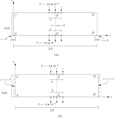
. Figure 1(a) and Figure 1(b) show schematics of the

plate, boundary conditions and loading for the formulation based on GM/WF for both simply supported and fixed-fixed boundary conditions. The load is applied over a length of

b

=

0.4

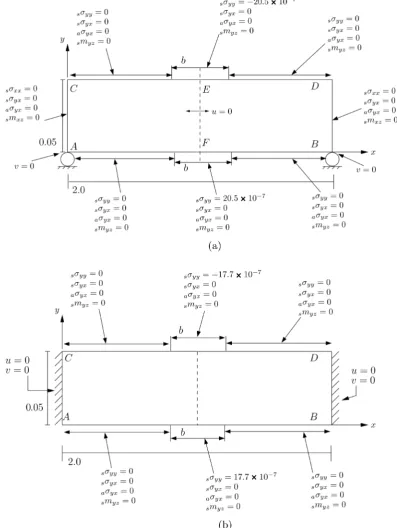
as forces at the nodes that corresponds to

uniform stress in the y-direction (see Figure 1). Figure 2(a) and Figure 2(b)

show same schematics with BCs and loading used in least squares formulation. In all numerical studies the plates are discretized using a 20 element uniform discretization (10 elements along the length and two elements width b) using a nine node p-version hierarchical higher order global differentiability finite elements. In all computations we choose Poisson’s ratio of 0.3, 0

6

ˆ

_{30 10}

E

=

E

= ×

psi, hence E=1, and 0≤ ≤α 0.25

 with

β

_ =0.0. α = 0 corresponds to

classical continuum theory. Progressively increasing values of

α

 produces

progressively more pronounced polar physics (resistance to deformation). Numerical solutions are calculated for the following:

1) For GM/WF we consider

k

=

3

(solutions of class 2

C in x and y) with

5

p= . For this choice of k, integrals over the spatial discretization are Riemann.

2) For GM/WF we also consider

k

=

2

(solutions of class 1

C in x and y)

with p=7. For this choice of k integrals over the spatial discretization are in

Lebesgue sense.

3) Since the solution for LSP yields residual functional values of the order of

(

15

)

10

(16)

confirm that when both solutions are almost indistinguishable from each other, the solution from GM/WF has good accuracy.

4) For Least squares formulation we consider solutions of class 0

C in x and y

with p-level of nine [40] [45].

Results GM/WF:

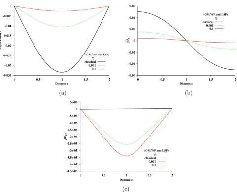
Figures 3(a)-(c) shows plots of v, iΘz and smxz versus x at y=0.025 (center line of the plate) for 0≤ ≤α 0.25

 . For α = 0 we have classical continuum

behavior. Progressively increasing values of

α

 results in progressively

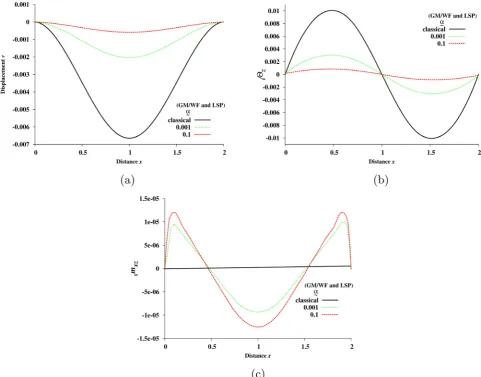
increasing resistance to deformation, hence progressively reducing displacement v, reducing rotation iΘz but increasing moment smxz. Similar graphs of v, iΘz and smxz versus x at y=0.025 for fixed-fixed plate are shown in Figures

4(a)-(c) for 0≤ ≤α 0.25

 . We observe similar behaviors of v, iΘz and smxz

[image:16.595.149.538.289.693.2]

(17)

[image:17.595.140.538.74.603.2]

Figure 2. Model Problem 1 and 2: Schematics, BCs and loading (dimensionless): LSP. (a) Simply suppported plate (b=0.4); (b) fixed-fixed plate (b=0.4).

with increasing

α

_{values. Due to clamped boundaries the displacement v is} significantly reduced and iΘz and smxz follow accordingly.

Comparison of results: GM/WF and LSP:

The numerical solutions obtained from LS formulation for exactly same BCs and loading (Figure 2) using local approximations of class 0

(18)

[image:18.595.101.496.65.358.2]

Figure 3. v,iΘz and smxz versus y=0.025: Simply supported plate (GM/WF). (a) v versus x at

0.025

y= ; (b) iΘz versus x at y=0.025; (c) smxz versus x at y=0.025.

Figure 4. v,_iΘ_z and _sm_xz versus y=0.025: Fixed-fixed plate (GM/WF). (a) v versus x at y=0.025; (b)

[image:18.595.100.498.397.691.2]

(19)

[image:19.595.60.542.61.452.2]

Figure 5. Simply supported plate: comparison of LSP and GM/WF. (a) v versus x at y=0.025; (b) iΘz versus x at y=0.025; (c) smxz versus x at y=0.025.

compared with those obtained using GM/WF ( 2

C solutions at p=5 or C1

solutions at p=7). In the LSP the residual functional for the discretization is of

the order

(

15

)

10

O − . This ensures that the computed solutions satisfy the

governing differential equations in the pointwise sense, hence the computed solutions are virtually same as the theoretical solution. Comparison of these solutions with GM/WF provides a check on the accuracy of the solutions obtained using GM/WF as in GM/WF there is no direct measure of accuracy in the method itself.

Figures 5(a)-(c) show the plots of v, iΘz and smxz versus x at y=0.025 for α =0

 , 0.001, and 0.1 (α = 0 being the classical theory) obtained using

GM/WF and a comparison with least squares method for simple supported plate. Similar results for GM/WF and a comparison with LSP for fixed-fixed plate are shown in Figures 6(a)-(c). In both Figure 5 and Figure 6, v, iΘz and smxz obtained using GM/WF and LSP are in perfect agreement with each other for all three values of

α

(20)

[image:20.595.58.540.69.446.2]

Figure 6. Fixed-fixed plate: comparison of LSP and GM/WF. (a) v versus x at y=0.025; (b) iΘz versus x at y=0.025; (c) smxz versus x at y=0.025.

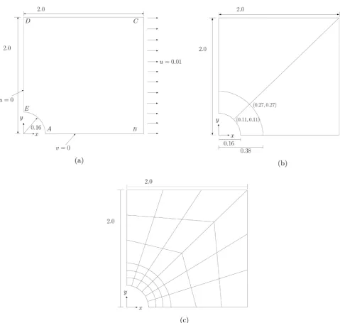
6.2. A Square Plate with a Circular Hole: Model Problem 3

We consider a 6" × 6" square plate of thickness 0.1" with a 0.48" diameter circular hole at the center. We use L0=1.5". The material properties, reference

quantities etc. used here are same as for model problems 1 and 2. Poisson’s ratio of 0.3 is used. This gives rise to a 4 4 0.06× × dimensionless plate with a hole

diameter of 0.16 (Figure 7(a)). The plate is subjected to uniform displacement of 0.01 (dimensionless) on its vertical faces that creates a uniform dimensionless stress field of

( )

σ

xx 0 =0.0048. The details of the BCs and loading for quarter

plate are shown in Figure 7(a). Figure 7(c) shows a graded discretization of the quarter plate. The plate is divided in four bicubic patches (Figure 7(b)). In each patch a 3 × 3 uniform discretization of nine-node p-version hierarchical elements with higher order global differentiability local approximation [59] [67] is used giving a total of 36 elements for the quarter of the plate. Computations are performed only using the formulation based on GM/WF with local approximation of class 1