Munich Personal RePEc Archive
Interest rates and endogenous population
growth: joint age-dependent dynamics
Brito, Paulo
Universidade de Lisboa, ISEG and UECE
27 March 2014
Online at
https://mpra.ub.uni-muenchen.de/58656/
Interest rates and endogenous population growth:
joint age-dependent dynamics
Paulo Brito
Universidade de Lisboa, ISEG and UECE
∗Preliminary draft, please do not quote
27.3.2014
Abstract
This paper presents a uncertain-lifetime overlapping-generations continuous time model for an Arrow-Debreu economy with endogenous fertility, in which age-dependent variables are explicitly introduced. The general equilibrium paths for the discount factor and newborns are derived from a system of two coupled forward-backward integral equations. The forward mechanism is re-lated to aggregation between cohorts and the backward mechanism to life-cycle decisions. We study changes in the age-dependent profiles of age-dependent dis-tributions for productivity and time use. We show that high maximum ages of productivity and child-rearing fitness increase the long run interest and growth rates, and low maximum ages can lead to asset pricing bubbles and negative population growth rates.
∗pbrito@iseg.utl.pt. Financial support from national funds by FCT (Funda¸c˜ao para a Ciˆencia
e a Tecnologia). This article is part of the Strategic Projects PEst.-OE/EGE/UI0436/2011 and
1
Introduction
What is the effect of ageing on interest rates ? How do interest rates react to age-dependent shocks ? More generally: what is the relation between demographics and interest rates ?
Some (rare) papers address the relationship between the age structure on the long run behavior of asset prices and interest rates. According to Fama (2006) and Favero et al. (2013) interest rates tend to follow moving average processes tending towards variable long run components associated to demography, and Geanakoplos et al. (2004) find that ratio young/middle is positively correlated with rates of interest. However, empirical studies do not offer a clear understanding of the mechanism between age-distribution of population and aggregate variables such as the interest rate. Overlapping-generations (OLG) models supply the available theory on the ef-fects (or joint determination) of demographics and asset markets. Most of the initial contributions, following Samuelson (1958), consider two- or three- period lifetimes. Attempts to extend these models to multiple period lifetimes (Auerbach and Kotlikoff (1987) and R´ıos-Rull (1996)) have only been solved numerically.
Is there a way to get an analytical understanding between asset prices and de-mography, and in particular, their joint responses to age-dependent shocks ?
lifetime OLG model of Yaari (1965) and Blanchard (1985) gave birth to a voluminous literature. However, most contributions have particular assumptions on demography that lead to the representation of equilibrium by ordinary differential equations, which simplifies the analysis at the cost of making it also unfit for studying changes in the profile of age-dependent densities.
Within the last strand of literature, some papers consider more general types of demography than in Blanchard (1985) implying a representation of equilibrium by integral equations. An earlier paper Cass and Yaari (1967), for a finite lifetime, OLG, production economy, found that equilibrium was represented by an integral equation. The integral equation representation was rediscovered recently in several endowment economy OLG models, of the finite lifetime strand, v.g. Demichelis and Polemarchakis (2007) and Edmond (2008). This is consistent with the observation by Santos and Bona (1989) the OLG models have a multiplicative operator nature.
In Brito and Dil˜ao (2010) we also found an integral equation representation of equilibrium in a infinite lifetime model, with a demography more general than in the existing Yaari (1965)-Blanchard (1985), allows for the study of age-dependent shocks. We considered uncertain lifetime with an infinite support (as in Yaari (1965)-Blanchard (1985)), an E−∞,∞ timing, an Arrow-Debreu1 endowment economy along
a growing balanced-growth path. Several age-dependent profiles of productivity were introduced and they all implied the same conclusion: for a log-utility function we proved that the long run real interest rate would increase for shifts in the income distribution such that the age of maximum income increases. The interest rate is the discount rate associated to Arrow-Debreu price, i.e, to prices for forward contracts in the good’s market. Given that the mass of the population was taken as exogenous, the supply and demand aggregate the members of cohorts according to their phase in their
1
particular life-cycles. Therefore, aggregate the age-distribution of supply and demand are determined by the life-cycle effect weighted by exogenous population densities. Then, intertemporal prices are associated essentially to a backward mechanism and their general equilibrium dynamics is governed by a double integral equation on AD prices.
In this paper endogenous fertility and endogenous population is introduced in the simplest way, through a version of the Barro and Becker (1989) fertility model 2 :
offsprings increase the utility of representative members of every cohort, but they also introduce a trade-off between time used to child-rearing and to work. We as-sume a production economy in which the only factor of production is labour, along a balanced growth path. Endogenous fertility and population dynamics introduce two main new feature to the model: first, as AD prices and fertility are jointly determined then the GE is represented by a system of two coupled integral equations, and, sec-ond, the market equilibrium condition is endogenously determined not only because it aggregates excess-demand or supply due to life-cycle decisions, but also because the population aggregators become endogenous. Then goods’ markets equilibria are de-termined by two types of endogenous dynamic effects: (i) by a life-cycle effect as in the exogenous population Brito and Dil˜ao (2010) model and (ii) by an endogenous aggre-gation effect because the aggregator, endogenous age-dependent population profiles, is also endogenous. Both dynamics can work in the same or in opposite directions and we prove that one of them tends to drive the asymptotic behavior of the interest rates and population3
2
There are other endogenous fertility papers in the finite-lifetime continuous-time literature. In
partial equilibrium context d’Albis et al. (2010) assume that the age of motherhood is endogenous.
3
In a way the the design of pension systems (PAYG or capitalisation) reflects the two
dimen-sions of heterogeneity introduced by age: heterogeneity along the life-cycle, within a cohort, or
Our approach allows for a parameterized analysis of some puzzling properties of OLG equilibrium models4: indeterminacy, in the sense that we have a continuum
equilibrium of equilibria (Samuelson (1958), Gale (1973)), endogenous fluctuations, rational asset pricing bubbles (Tirole (1985)).
The main results of the paper are the following: first, interest rates and population growth is driven by a life-cycle (anticipating) and a cohort aggregation (evolutionary) mechanisms; second, age-dependent distribution of productivity and child-rearing fitness determine the dynamics of both interest rates and the rate of growth of the population; third, there is indeterminacy for interest rates (and depending on the version, for the rate of growth); fourth, the aggregate (life-cycle) effect dominates if the age of maximum productivity is high (low) and the age of maximum fertility is low (high); and , fifth, asset pricing bubbles can occur if productivity and fertility maxima are reached earlier in the lifetime, and, in this case, population tends to growth asymptotically at negative rates.
The paper unfolds as follows. In section 2 the model’s components are described and the general equilibrium system of integral equations is presented, In section 3 we solve the equilibrium integral equations for two, age-independent and age-dependent, distribution. Section 4 concludes.
2
The model
This paper introduces the following assumptions as regards demographics technology, and the institutional framework. At each point in time a new cohort borns, the size of thew cohort depends on age-distribution of the population and on the distribution of the fertility rate, which is also age-dependent. The lifetime for each cohort is
uncer-4
The basic reason for those properties is related to the lack of market equilibrium at infinity (see
tain, and we take it at infinite. However, the size of every cohort decays exponentially by the mortality rate. Along its lifetime, the members of the cohort consume, work and have offspring and all those activities are age-dependent, and their resources come from the labor income. All the individual within every cohort are homogeneous.
We assume an Arrow-Debreu economy in which there are only product markets opening at the ”Archimedian time” t = −∞. At this date, there is a spot market and an infinite number of forward markets for delivery at any future date individual members of every cohort, irrespective of the time of birth, take those prices as given. All the individual members of every cohort may only perform spot and forward transactions at the time of birth,t0, at prices consistent to those set att=−∞. As we
assume that there are intergenerational transfers, every member of all cohorts should face an intertemporal budget constraint taking the Arrow-Debreu price as given. The preferences are characterized by an additive intertemporal utility functional, depending upon consumption and the number of children. Child-rearing have a cost in time spent depending on the number of children and the age of the parent by a fitness factor.
We consider a production economy, in which labor is the only endogenously deter-mined factor of production but having an age-dependent productivity, growing along a balanced growth path (BGP).
In this age-dependent model, the main functions are age-dependent densities. We introduce the endogenously determined densities for fertility and population, con-sumption, wage income and, implicitly, savings. We consider two exogenous densities related to child-rearing fitness and productivity.
life-cycle arbitrage condition, and, second, the endogenous fertility choice also determines the density of population and, therefore, the aggregator. The first is anticipative and forward-looking and the second is evolutionary, backward-looking. The two mecha-nisms therefore, tend to operate simultaneously. However, depending on the initial conditions and on the parameters of the model one of them tends to be dominant.
2.1
Demographics
To describe the growth of population during time, we follow the age-structured McK-endrick model, McKMcK-endrick (1926). We denote by n(a, t) the density of individuals of a population with age a≥0 and at time t. The aggregate population is
N(t) =
+∞
Z
0
n(a, t)da. (1)
The evolution of the density of individuals of an age-structured population can be simply described by the first order partial differential equation,
∂n(a, t)
∂t +
∂n(a, t)
∂a =−µ(a)n(a, t) (2)
where µ(a) is the age-dependent mortality rate of the population. We assume mor-tality is time-independent. The new-borns are introduced through the boundary condition,
b(t)≡n(0, t) =
Z +∞
0
β(a, t)n(a, t)da (3) where β(a, t) is the fertility density of age a at time t.
The population density at timetis determined from the initial population density,
n(a, t = 0) =ψ(a), witha, t ∈R+.
solution on each characteristic curve as5
n(a, t) =n(a0, t0)e
−Rt
t0µ(s+a0−t0)ds. (4)
The individuals of a population that were born around some timet =t0is acohort
of the population, and (4) relates the density of individuals in the same cohort. Let
t0 be the (universal) time at which a cohort is born. The initial size of a cohort
is b(t0) = n(0, t0) and is related to the density of the existing cohorts by b(t0) =
R+∞
0 β(a, t0)n(a, t0)da and the size of a cohort born at time t0, at time t = a+t0,
where its members are of age a is n(a, t0+a) = b(t0)π(a) where
π(a)≡e−R0tµ(a)da (5)
is the instantaneous probability of survival for at age a.
2.2
Representative agent of cohort
t
0The number of offspring produced by the cohort t0, up to time t≥t0 is
Z t
0
β(s, t0+s)n(s, t0+s)ds =b(t0)
Z t
0
β(s, t0+s)e−
Rs
0 µ(z)dzds.
Then the number of children by a member of the cohort produced during its lifetime is
Z ∞
0
β(a, t0+a)e−
Ra
0 µ(s)dsda.
We assume that consumers have a von-Neumann-Morgenstern utility function displaying impatience and uncertain lifetimes where the the probability of survival is age-dependent but cohort-independent.
We also assume that agents derive utility both from consumption and from the joy to parenting. A particular logarithmic instantaneous utility function is assumed
U(t0) =
Z ∞
0
ln(c(a, t0+a)) +φln(β(a, t0+a))R(a)π(a)da (6)
5
where φ weights the relative felicity derived from consumption and from parenting and is assumed to be independent from age and
R(a)≡e−Ra
0 ρ(s)ds
is the psychological discount factor where ρ(.)≥0
We assume a production economy in which there is a single good which is not stored and is used in consumption. The production economy uses only one input, labor, with a linear technology
y(a, t) =A(a, t)l(a, t)
where A(.) is the average and marginal productivity of labor and l(.) is the time dedicated to production.
We assume a production economy in which there is a single good which is not stored and is used in consumption. Production uses only one input, labor, with a linear technology
y(a, t) =A(a, t)l(a, t)
where A(.) is the average and marginal productivity of labor and l(.) is the time dedicated to production.
We follow Becker and Barro (1988) by assuming that the major cost of child-rearing is the time lost to production. We assume that the time spend per-child is a linear function of the number of children v(a)β(a, t) wherev(a) is a fitness coefficient which is age dependent.
If we normalize the total time to 1 then the time-use balance equation is
l(a, t) +v(a)β(a, t) = 1,
We assume that a complete asset market exists, in which Arrow-Debreu contracts may be performed, as in Brito and Dil˜ao (2010). There is an Arrow-Debreu contract for delivery of one unit of the good at price p(t). The price is consistent between cohorts and is set at the ’Archimedian” time t =−∞. This allows agents to allows members of every cohort to perform life-cycle allocations of net income, at the time of birth t0.
Then the stock of human wealth, or the value at time of birth of the lifetime labor income, for a member of cohort t0, is
h(t0)≡
Z ∞
0
p(t0+a)y(a, t0+a)π(a)da
where y(a, t0+a) = A(a, t0+a)(1−v(a)β(a, t0 +a)).
Therefore, the problem for the representative member of the cohort born at t0,
Pad:
max
(c(a,t0+a),β(a,t0+a))a∈[0,∞) Z ∞
0
ln(c(a, t0+a)) +φln(β(a, t0+a))R(a)π(a)da
subject to the intertemporal budget constraint
Z ∞
0
p(t0+a)(1−v(a)β(a, t0+a))A(a, t0+a)−c(a, t0+a))π(a)da = 0, (7)
for (c(a, t), β(a, t))∈Ω(t0), where
Ω(t0)≡ {(c(a, t0+a), β(a, t0+a)) :c(a, t0+a)>0, 0< v(a)β(a, t0+a)<1, for alla∈R+}.
We introduce two magnitudes: the maximum wealth that cohort t0 can get
¯
h(t0)≡
Z ∞
0
p(t0+a)A(a, t0+a)π(a)da (8)
which occurs if cohort t0 is childless, and the average lifetime discount factor
¯
R≡ Z ∞
0
Lemma 1. The optimal consumption and fertility for a member of cohort t0 with age
a∈[0,∞) are
c∗
(a, t0+a) =
R(a)
p(t0+a)
¯
H(t0)
(1 +φ) ¯R, a∈[0,∞) (10)
and
β∗
(a, t0+a) =
R(a)
p(t0 +a)v(a)A(a, t0+a)
φH¯(t0)
(1 +φ) ¯R, a∈[0,∞) (11)
where (c∗(a, t
0+a), β∗(a, t0+a))∈Ω(t0).
Consumption, for any moment along the lifetime of a member of cohort t0 is
proportional to the lifetime human wealth. The age-dependency is captured by the ratio R(a)/p(t0 +a), the ratio between the cohort and the market discount factor,
as in the exogenous-fertility model (see Brito and Dil˜ao (2010)). The fertility rate at age a is proportional to consumption, because
β∗
(a, t0+a) = φ
c∗
(a, t0+a)
v(a)A(a, t0+a)
a∈[0,∞).
However, the proportionality is age-dependent: it decreases with both productvity and the fitness to child-rearing. Therefore, fertility has two economic components and a biological one (translated byv(.)). We find that an increase in average productivity has two effects on fertility: (a) a substitution effect diminishes fertility, while (b) a wealth effect, by increasing human capital, increases fertility.
2.3
Aggregation
Taking t > a in equation (4) we have the density of individuals of age a at timet
n(a, t) =n(0, t−a)e−R0aµ(s)ds. (12)
where b(t) =n(0, t) is the number of newborns at time t. The number of newborns is endogenous
b(t) = n(0, t) =
Z ∞
β∗
(a, t)n(a, t)da=
Z ∞
β∗
(a, t)b(t−a)e−Ra
where β∗
(.) is given by equation (11). The total population is
N(t) =
Z ∞
0
n(a, t)da=
Z ∞
0
b(t−a)e−R0aµ(s)ds
da (14)
We take the initial population N(0) = R∞
0 b(−a)e
−R0
−aµ(z)dzda=N
0 as given.
The aggregate demand for goods is
C(t) =
Z ∞
0
c∗
(a, t)n(a, t)da=
Z ∞
0
c∗
(a, t)b(t−a)e−R0aµ(s)ds
da (15) where c∗
(.) is given by equation (10), and the aggregate supply is
Y(t) =
Z ∞
0
(1−v(a)β∗
(a, t))A(a, t)n(a, t)da =
Z ∞
0
(1−v(a)β∗
(a, t))A(a, t)b(t−a)e−R0aµ(s)dsda
(16) In the last case, the fertility rate affects both the density of output per age but also the aggregator.
2.4
General equilibrium
Definition 1. The OLG-Arrow-Debreu general equilibrium Is defined by the
densities(c(a, t))(a,t)∈R2
+, (β(a, t))(a,t)∈R2+ and the paths(p(t))t∈R+ and(b(t))t∈R+ such
that, given the initial population N0: (i) agents optimize c(a, t) = c∗(a, t), β(a, t) =
β∗
(a, t)solvePad, (ii) the equilibrium condition for the good’s market is ,C(t) = Y(t)
holds (iii) the endogenous number of newborns isb(t) = R∞
0 β
∗(a, t)b(t
−a)e−R0aµ(a
′
)da′da
As we saw in Brito and Dil˜ao (2010), the system of spot and forward markets operating at time of birth of any cohort should be consistent irrespective of t0. Then
we may consider that markets operate at t = 0 and consider all the variables as discounted values as regards t= 0.
Setting t=t0+a then we can rewrite equations (10) and (11) as
c∗
(a, t) = R(a)¯h(t−a)
and
β∗
(a, t) = φ¯h(t−a)R(a)
(1 +φ)p(t)A(a, t) ¯R, a∈[0,∞) (18)
where
¯
h(t−a)≡
Z ∞
0
p(t−a+s)A(s, t−a+s)π(s)ds. (19) If we substitute the the optimal consumption and fertility, equations (17) and (18) in the market clearing equation whereC(t) and Y(t) are given by equations (15) and (16), respectively, we get the equilibrium equation for the AD prices
p(t) = 1¯
R R∞
0 n
∗
(a, t) ¯H(t−a)R(a)da R∞
0 n
∗(a, t)A(a, t)da , (20)
where n(a, t) is the equilibrium density of population in equation (12)
Substituting the equilibrium fertility rate, in equation (18), into the equilibrium birth rate equation (13) we get,
b(t) = φ (1 +φ) ¯Rp(t)
Z ∞
0
¯
H(t−a)b(t−a)π(a)R(a)
v(a)A(a, t) da
Therefore, the general equilibrium is characterized by the pair of functions p(t), b(t) for t∈R+ which solve the system of integral equations
p(t) = 1¯
R R∞
0
R∞
0 b(t−a)p(t−a+s)A(s, t−a+s)π(s)π(a)R(a)dsda
R∞
0 b(t−a)A(a, t)π(a)da
, (21)
b(t) = φ (1 +φ) ¯R
Z ∞
0
Z ∞
0
p(t−a+s)A(s, t−a+s)π(s)b(t−a)π(a)R(a)
p(t)v(a)A(a, t) dsda(22) given the initial total population is given N(0) = N0.
The solution depends upon the age-dependent functions µ(a), ρ(a), v(a) and
2.5
Balance growth path
In order to get some qualitative results, we restrict the analysis to the balanced growth paths (BGP), that is to separable but age-dependent productivity densities,A(a, t) =
A(a)eγt, to constant rate of time preference and mortality rates, ρ(a) = ρ > 0 and
µ(a) =µ > 0. Therefore the unique exogenous age-dependent forcing functions are
A(a) and v(a). The system of integral equations (21)-(22) becomes
p(t) =
R∞
0
R∞
0 p(t−a+s)b(t−a)K0(a, s)ds da
R∞
0 b(t−a)K1(a)da
(23)
p(t)b(t) =
Z ∞
0
Z ∞
0
b(t−a)p(t−a+s)K2(a, s)ds da (24)
where the kernels are
K0(a, s) = (ρ+µ)A(s)e−(µ−γ)se−(γ+ρ+µ)a
K1(a) = A(a)e−µa
K2(a, s) =
φ
1 +φ
K0(a, s)
A(a)v(a). The kernels should be L1(
R+) functions and are of the backward-forward type: the
forward term,s, is related to thelife-time planning nature of the consumer’s problem, irrespective of the cohort, the backward term a is related to the aggregation among existing cohorts.
The equilibrium (real) interest rate and the rate of growth of population can be obtained from the solutions of equations (23) and (24) as r(t) = −p˙(t)/p(t) and
η(t) = ˙N(t)/N(t), respectively.
If the kernels K0, K1 and K2 are continuous, the solution should be unique. We
use the Wiener-Hopf approach with the eigenfunction expansions
p(t) =X
k
p0ke−rkt, b(t) =
X
l
where rk and λl are complex numbers and p0k and b0l are arbitrary constants. The
eigenfunctions r and λ are the solutions of the characteristic system:
Z ∞
0
A(a)e−(λ+µ)a
1−ρ+µ
λ −r+γ+ρ+µe
−(r−γ−λ)a
da = 0 (25) and
(ρ+µ)φ
1 +φ Z ∞
0
Z ∞
0
A(s)
v(a)A(a)e
−(λ−r+γ+ρ+µ)ae−(r+µ−γ)sdsda= 1 (26)
If we can determinep(.) andb(.) then we can obtain the equilibrium consumption and fertility densities from
c(a, t) = (ρ+µ)¯h(t−a) (1 +φ)p(t) e
γte−(γ+ρ)a
and
β(a, t) = (ρ+µ)φ¯h(t−a) (1 +φ)v(a)A(a)p(t)e
−(γ+ρ)a.
To characterise further the equilibrium we introduce assumptions regarding the distributionsA(a) andv(a). We start with age-independent function and next intro-duce Mincerian densities.
3
Applications
3.1
Particular case: age-independent densities
To start with the simplest case, we assume in this section an uniform distributions for productivity, A(a) =A0 >0, and time-use, v(a) = v0 >0.
Lemma 2. (Equilibrium price and birth rate) Letη≡β0−µ andβ0 ≡φ/(v0(1 +φ))
the number of newborns verifies
b(t) = b0eηt, t∈[0,∞) (27)
p(t) = p0,1e−ρt+p0,2e−ηt
e−γt
, t∈[0,∞) (28)
where b0 =β0N0 and p0,1 and p0,2 are arbitrary constants.
In this simple version of the model, the determination of the population dynamics and of the Arrow-Debreu prices can be done recursively. The number of newborns grows at the rate of population growth. This is equal to the endogenous fertility rate, which is driven by the trade-off between the love for parenting and the time withdrawn from production to rearing them, less the mortality rate. The total population is
N(t) = b(t)µ . If we calibrate with data for the U.S we would getb(t)/N(t)≈0.0127×2 to which corresponds an the average age E(a) = 1
µ ≈ 40 years. Historical data
suggests the second dominates: ρ > η.
The dynamics of Arrow-Debreu prices display three effects: first, if output grows at the rate γ along the BGP the increase in supply drives process down; second , there a life-cycle discounting effect (working through theρterm); and, third, there is the aggregative (working throughη) which is a result of the increase in supply driven by the increase in the mass of population. Under the assumptions in Lemma 2, we haveρ > η which implies that the aggregative effect dominates the life-cycle effect.
We can see more clearly how these effects operate by studying the equilibrium fer-tility density and the interest rate. The equilibrium endogenous ferfer-tility rate density also displays the two (life-cycle and aggregative) effects
β(a, t) = β0p0,1 + (ρ+µ)p0,2e
(ρ−η)(t−a)
p0,1+β0p0,2e(ρ−η)t
The admissibility constraint 0< β(a, t)v0 <1 holds ifβ0 < µ+ρ≤ v10 or, equivalently,
decreasing in age. The equilibrium population can increase or decrease through time, depending on the sign of η.
The DGE interest rate is
r(t) =
η+γ, if η=ρ
(ρ+γ)(η+γ−r0)−(η+γ)(ρ+γ−r0)e−(η−ρ)t
(η+γ−r0)+(r0−γ−ρ)e−(η−ρ)t , if η6=ρ
(29)
Proposition 1. Let the assumptions in Lemma 2 hold. Then, along a BGP, the
interest rate is non-stationary and tends asymptotically to γ+η. The time t= 0 level of the interest rate in indeterminate, but has to verify r0 < η+γ < ρ+γ.
We say there are speculative bubbles if r(∞)<0. In our model we have specula-tive bubbles if γ+η <0 independently of the rate of growth of the population. This seems to be unrealistic given the data.
3.2
Particular case: age-dependent densities
We now assume age-dependent densities productivity and fitness in rearing children, in terms of time use. In particular, we introduce Mincerian distribution for the age-density of productivity per unit of time spent in production
A(a) = A0eαa(Ka−a), α >0, A0 >0 (30)
whereKa/2 = age of maximum productivity (US: α≈0.00156,Ka ≈109.3). We are
assuming that productivity is increasing up to age Ka/2 and decreases later in the
lifetime. However, the output profile per age depends not only on the (exogenous) profile of productivity but also on the (endogenous) time allocated to production.
We also assume an inverse Mincerian age-profile for fitness in child-rearing
where Kv/2 = the age of maximum fitness (Kv ≈ 56). The fitness in child-rearing,
which is the inverse of time spending, increases up to age Kv/2 and increases
after-wards. However, the fertility profile per age depends not only on the (exogenous) fitness but also other (endogenous) factors like human wealth.
Next we introduce two functions on x=r−γ and λ, Ψ(k) = Ψ(k, Ka)≡
√
π
2√αe
z2
erfc(z), z≡ k+µ−αKa
2√α , k=x, λ (32)
and ˜
Ψ(λ−x) = ˜Ψ(λ−x, Ka, Kv)≡
√
π
2√ν−αe
˜
z2erfc(˜z), z˜
≡ λ−x+ρ+µ+αKa−νKv
2√ν−α
(33) where
erfc(x) = 1−erf(x) = √2
π Z ∞
x
e−y2 dy.
We define the critical magnitudes
ξ =ny: β0(ρ+µ)Ψ(z(y)) ˜Ψ(0) = 1
o
(34) and
ξ∗
= 2α
Ka
2 − 1
ρ+µ
+β0(ρ+µ) ˜Ψ(0)−µ. (35)
We emphasise the fact that ξ∗
= ξ∗
(Ka, Kv) only depends on parameters, and, in
particular on Ka and Kv, as ˜Ψ(0) is a function of them both. We also introduce the
following function
s(Ka, Kv)≡(ρ+µ)Ψ
′
(ξ∗
(Ka, Kv)) + Ψ(ξ∗(Ka, Kv)).
We introduce the following one-dimensional manifold over the domain of (Ka, Kv),
K ⊂R2++,
This set partitions set K into two subsets
K+={(Ka, Kv)∈ K: s(Ka, Kv)>0}
and
K− ={(Ka, Kv)∈ K: s(Ka, Kv)<0}.
Lemma 3. Assume that ν > α. Then the general solution for the integral system is:
1. if (Ka, Kv)∈S
p(t) = p0,ξe−(ξ
∗+γ)t
b(t) = b0,ξeξ
∗t
2. if (Ka, Kv)∈/ S
p(t) = p0,ξe−(ξ+γ)t+p0,ξ−e
−rξ−t
b(t) = b0,ξeξt+b0,ξ−e
λξ−t
where ξ > ξ∗
and rξ− −γ < ξ < λξ− if (Ka, Kv) ∈ K+, and ξ < ξ
∗
and
rξ− −γ > ξ > λξ− if (Ka, Kv)∈ K−.
Again, there is indeterminacy as far as the AD price is concerned because the initial value of the prices is not pinned down by the model. If (Ka, Kv) ∈/ S there is
also indeterminacy regarding because we only know b0 =b0,ξ+b0,ξ−
The general solution for the interest rate is
r(t) = (ξ+γ)(r0−γ−xξ−) + (xξ−+γ)(ξ+γ−r0)e
−(xξ−−ξ)t
r0−γ−xξ−+ (ξ+γ−r0)e
−(xξ−−ξ)t
Lemma 4. Let (Ka, Kv)∈/ S. Then, the interest rate:
1. is stationary in the cases
r(t) =
ξ+γ, ifr0 =ξ+γ
xξ−+γ, ifr0 =xξ−+γ
2. it is non-stationary in the cases:
lim
t→∞r(t) =
xξ−+γ, ifr0 < ξ+γ andxξ− < ξ
ξ+γ, ifr0 < xξ−+γ andxξ− > ξ
The solution for the rate of growth of the population
η(t) = ξ(λξ−−η0)−λξ−(ξ−η0)e
(λξ−−ξ)t
(λξ−−η0)−(ξ−η0)e
(λξ−−ξ)t
for λξ− 6=ξ and η0 is the initial rate of population growth. Lemma 5. Let (Ka, Kv)∈/ S Then the rate of population growth:
1. is stationary in the cases
η(t) =
ξ, ifη0 =ξ
λξ−, ifη0 =λξ−
2. it is non-stationary in the cases:
lim
t→∞η(t) =
ξ, ifη0 > λξ− andλξ− < ξ
λξ−, ifη0 > ξ, andλξ− > ξ
Lemma 6. Let (Ka, Kv)∈/ S. Then:
1. the aggregation effect dominates ifλξ− < ξ < xξ−, and η0 > λξ− and r0 < ξ+γ
lim
t→∞r(t) =ξ+γ, tlim→∞λ(t) =ξ
2. the lifetime effect dominates if λξ− > ξ > xξ−, and η0 > ξ and r0 < xξ−+γ
lim
t→∞r(t) = xξ− +γ, tlim→∞λ(t) =λξ−
The case in which the aggregate effect dominates was the only one that was possible when we had age-independent productivity and child-rearing fitness. This case is sometimes called the asymptotic golden rule case, and the asymptotic rate of interest is equal to the rate of productivity growth plus the population growth.
With Mincerian age-dependent functions a domination of lifetime effect is also possible. In this case, sometimes labeled the inefficient steady state, the asymptotic interest rate is smaller than the sum of the rate of growth in productivity plus the rate of growth of the population and the rate of growth of population is relatively higher than in the asymptotic golden rule.
We introduce the sets (one-dim manifolds), associated to the non-increasing in population
K0 ={(Ka, Kv) : ξ(Ka, Kv)≤0}
and associated to the emergence bubbles r≤0
K−γ{(Ka, Kv) : ξ(Ka, Kv) =−γ}
We can also define the corresponding sets (zero-dim manifolds) over S, associated to zero population growth rate S0 = {(Ka, Kv)∈S : ξ∗(Ka, Kv) = 0} and to the
Proposition 2. Let (Ka, Kv)∈ K. Then four main cases are possible:
1. if there is a high Ka and a low Kv then rate of interest will converge to the
asymptotic golden rule level and population growth will be positive
asymptoti-cally;
2. if there is a low Ka and a highKv then rate of interest will converge to the
in-efficient steady level state and population growth will be positive asymptotically;
3. if there are both low Ka and Kv then there will be asymptotic rational bubbles
and population decline
4. if there are high Ka and Kv there will asymptotic golden rule or inefficient
steady state and population growth.
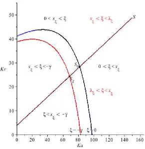
Figure 1 presents a bifurcation diagram, in space (Ka, Kv) for the partition of set
K illustration proposition 2: below line S the aggregation effect dominates, above line S the lifetime effect dominates, below line ξ = 0 population declines and below line ξ =−γ there will be asymptotically rational asset pricing bubbles.
4
Conclusions
third, rational bubbles can occur and are associated with negative population growth rates, which occur when both the ages for maximum productivity and fertility are low.
References
Auerbach, A. J. and Kotlikoff, L. J. (1987). Dynamic Fiscal Policy. Cambridge University Press.
Barro, R. J. and Becker, G. S. (1989). Fertility choice in a model of economic growth.
Econometrica, 57(2, March):481–501.
Becker, G. S. and Barro, R. J. (1988). A reformulation of the economic theory of fertility. Quarterly Journal of Economics, 103(1, February):1–25.
Blanchard, O. J. (1985). Debt, deficits and finite horizons. Journal of Political Economy, 93(2):223–47.
Bommier, A. and Lee, R. D. (2003). Overlapping Generations Models with Realistic Demography: Statics and Dynamics. Journal of Population Economics, 16:135–60. Boucekkine, R., de la Croix, D., and Licandro, O. (2002). Vintage Human Capi-tal, Demographic Trends and Endogenous Growth. Journal of Economic Theory, 104(2):340–75.
Brito, P. (2008). Equilibrium asset prices and bubbles in a continuous time olg model. MPRA Paper 10701, Munich Personal RePEc Archive.
Cass, D. and Yaari, M. E. (1967). Individual saving, aggregate capital accumulation, and efficient growth. In Shell, K., editor,Essays on the Theory of Optimal Economic Growth, pages 233–268. MIT Press.
Cushing, J. M. (1998). An introduction to structured population dynamics. SIAM, Philadelphia.
d’Albis, H. and Augeraud-Veron, E. (2007). Competitive growth in a life-cycle model : existence and dynamics. available at http://ideas.repec.org/p/mse/wpsorb/v04016.html.
d’Albis, H. and Augeraud-V´eron, E. (2009). Competitive growth in a life-cycle model: existence and dynamics. International Economic Review, 50(2):459–484.
d’Albis, H., Augeraud-V´eron, E., and Schubert, K. (2010). Demographic-economic equilibria when the age at motherhood is endogenous. Journal of Mathematical Economics, 46(6):1211–1221.
Demichelis, S. and Polemarchakis, H. M. (2007). The determinacy of equilibrium in economies of overlapping generations. Economic Theory, 32(3):471–475.
Dil˜ao, R. (2006). Mathematical models in population dynamics and ecology. In Misra, J. C., editor,Biomathematics: Modelling and Simulation. World Scientific.
Edmond, C. (2008). An integral equation representation for overlapping generations in continuous time. Journal of Economic Theory, 143(1):596–609.
Favero, . C. A., Gozluklu, . A. E., and Yang, . H. (2013). Demographics and The Behavior of Interest Rates. Working Papers wpn13-10, Warwick Business School, Finance Group.
Gale, D. (1973). Pure exchange equilibrium of dynamic economic models. Journal of Economic Theory, 6(1):12–36.
Geanakoplos, J. (2008). Overlapping generations models of general equilibrium. Dis-cussion Paper 1663, Cowles Foundation for Research in Economics, Yale University. Geanakoplos, J., Magill, M., and Quinzii, M. (2004). Demography and the long-run predictability of the stock market. Brookings Papers on Economic Activity, 1:241–307.
Gelfand, I. M. and Fomin, S. V. (1963). Calculus of Variations. Dover.
McKendrick, A. G. (1926). Applications of mathematics to medical problems. Pro-ceedings of the Edinburgh Mathematical Society, 44:98–130.
Polyanin, A. D. and Manzhirov, A. V. (2008). Handbook of Integral Equations. Chap-man & Hall, 2nd edition.
R´ıos-Rull, J.-V. (1996). Life-cycle economies and aggregate fluctuations. Review of Economic Studies, 63:465–489.
Samuelson, P. A. (1958). An Exact Consumption-Loan Model of Interest with or Without the Social Contrivance of Money.Journal of Political Economy, 66(6):467– 82.
Tirole, J. (1985). Asset bubbles and overlapping generations. Econometrica, 53(6):1499–1528.
Webb, G. F. (1985). Theory of Nonlinear Age-Dependent Population Dynamics. Mar-cel Dekker Inc., New York.
Yaari, M. E. (1965). Uncertain lifetime, life insurance, and the theory of consumer.
A
Appendix: Proofs
Proof of Lemma 1. The problem Pad is a isoperimetric problem, which we can solve
using calculus of variations techniques. We define the Lagrangean as
L(c, β, q) =
Z ∞
0
ln(c(a, t0 +a)) +φln(β(a, t0+a))R(a)π(a)da+
+q Z ∞
0
p(t0+a)(1−v(a)β(a, t0+a))A(a, t0+a)−c(a, t0+a))π(a)da
(37) where q is the Lagrange multiplier. Let us assume there are functions c(a, t0 +a)
and β(a, t0+a) in Ω(t0) maximise L. Necessary conditions for an interior optimum
are
∂L ∂q = 0,
δL
δc = 0, and δL δβ = 0
where ∂/∂q is a standard derivative and δ/δc and δ/δβ are functional derivatives. Using a standard definition (Gelfand and Fomin, 1963, p. 12), we introduce two arbitrary functions ǫc(a) and ǫβ(a) both in L1(R), and introduce a parameterized
perturbations ¯c(a, t0+a) =c(a, t0+a) +αǫc(a) and ¯β(a, t0+a) = β(a, t0+a) +αǫβ(a)
over the solution of the problem, where α is a parameter. The functional derivatives of L are defined as
δL(c, β)
δc =
δL(¯c,β¯)
δc α=0
, δL(c, β) δβ =
δL(¯c,β¯)
δβ α=0 . We get δL δc = Z ∞ 0
R(a)
c(a, t0+a)−
qp(t0+a)
π(a)ǫc(a)da (38)
δL δc =
Z ∞
0
φ R(a) β(a, t0+a) −
qp(t0+a)v(a)A(a, t0 +a)
π(a)ǫǫ(a)da (39)
As c(a, t0 +a) and β(a, t0+a) are maximisers for the Lagrangean the equalities 38
the parentheses must be zero for all a ∈R+. Then we get the optimal consumption
and fertility for every age of the member of cohort t0
c∗
(a, t0 +a) =
R(a)
qp(t0+a)
(40)
β∗
(a, t0 +a) =
φR(a)
qp(t0+a)v(a)A(a, t0+a)
(41) If we introduce these functions into the intertemporal budget constraint, (7) we get the Lagrange multiplier
q= (1 +φ)¯R¯
h(t0)
.
where ¯ht0 and ¯R are defined in equations (8) and (9), respectively. Substituting q
into equations (40) and (41) we get the optimal consumption and fertility functions (10) and (11). If h(t0) > 0 and if prices and productivity are positive, p(.) > 0 and
A(.), then c∗
(a, t0+a) > 0 and β∗(a, t0 +a) > 0 for every a ∈ R+. The condition
v(a)β∗
(a, t0+a)<1 is equivalent toφR(a)¯h(t0)<(1 +φ)p(t0+a)A(a, t0+a) ¯R which
can be checked at the GE level.
Proof of Lemma 2. In this case then equations (21) and (22) become a the recursive system
b(t) = β0
Z ∞
0
Z ∞
0
b(t−a)e−µada (42)
p(t) = (ρ+µ)
R∞
0 b(t−a)p(t−a+s)e
−(µ−γ)se−(µ+ρ+γ)adsda
R∞
0 b(t−a)e
−µada (43)
(44) Using a solution method for similar equations in (Polyanin and Manzhirov, 2008, p.381), the general solution may be a linear combination of eigenfunctions having the form
p(t) =X
k
p0ke−rkt, b(t) =
X
l
where rk and λl are the roots, in general complex roots of a system of characteristic
equations to be determined next. As the system (43)-(42) is recursive, we set b(t) =
b0e(λr+λci)t in the linear integral equation (42) and get the characteristic equation
1 = β0
Z ∞
0
e−(λr+µ+λci)ada=
= β0
Z ∞
0
e−(λr+µ)a(cos (−λ
ca) + sin (−λca)i)da.
The integration is well defined only if λr +µ > 0, which leads to the equivalent
characteristic equation
1 =β0
λr+µ−λci
(λr+µ)2+λ2c
.
(observe that, for the complex conjugate root λr−λci we would get the complex
conjugate equation). Then, the solution for λr and λc can be obtained from
β0(λr+µ)
(λr+µ)2+λ2c
= 1
−(λ β0λc
r+µ)2+λ2c
= 0.
As β0 > 0 then we have a single root λc = 0 and λr = β0 −µ, that verifies the
conditions λr+µ=β0 >0. Then the general solution for equation (42) is
b(t) = b0e(β0−µ)t. (46)
If we substitute this solution in equation (43) we get the linear integral equation for onp(t)
p(t) = (ρ+µ)β0
Z ∞
0
p(t−a+s)e−(µ−γ)se−(ρ+γ+β0)adsda. (47)
Trying p(t) =p0e−(rr+rci)t, we get the characteristic equation
1 =(ρ+µ)β0
Z ∞
0
Z ∞
0
e−(µ−γ+rr+rci)se−(ρ+γ+β0−rr−rci)adsda=
=(ρ+µ)β0
Z ∞
0
Z ∞
0
e−(µ−γ+rr)se−(ρ+γ+β0−rr)a[ cos (−r
ca) cos (−rcs)−sin (−rca) sin (−rcs)+
The equation is well defined only if −µ < rr−γ < ρ+β0. Under this condition, the
characteristic equation becomes
[(µ−γ+rr)2+r2c][(γ+ρ+β0−rr)2+r2c]
β0(ρ+γ)
= (µ−γ+rr)(γ+ρ+β0−rr)−r2c+rc(β0+µ+ρ)i
Asβ0+µ+ρ >0 thenrc = 0, thenrris the root of equation (µ+rr−γ)(γ−rr+ρ+β0) =
β0(µ+ρ), that has two roots r1 =γ +ρ and r2 =γ+β0−µ. Both roots verify the
conditions −µ < rj−γ < ρ+β0 for j = 1,2 as ρ > 0, µ >0 and β0 >0. Then the
general solution of equation (43) is
p(t) = p0,1e−(γ+ρ)t+p0,2e−(β0−µ−γ)t (48)
Equations (46) and (48) are candidate solutions, we have to check if the are admissible. First, we have to verify if the consumption and fertility decisions for every cohort are admissible, i.e, if (c(a, t), β(a, t)) ∈ Ω(t −a). We find c(a, t) = vA
φ e γtl(t
−a) and
v(a)β(a, t) =l(t−a) where l(t−a)≡ vβ0+(ρ+µ)π0e−(β0−ρ−µ)(t−a)
1+π0e−(β0−ρ−µ)(t−a)
and π0 =p2,0/p1,0.
Then sufficient conditions for admissibility are: π0 >0, which implies that bothc(a, t)
and l(t−a) are positive for all t ∈ R+ and β0 < ρ+µ < 1/v which, together with
π0 >0, implies that l(t−a)<1 for alla≥0. Second, we can determine b0 from the
initial data on populationN(0) =R∞
0 n(0, a)da=
R∞
0 b0e
−β0ada=b
0/β0 =N0.
Proof of proposition 1. Consider equation 29. It displays no singularities (thatr(t) =
∞ for a finite t) if r0 ≤ max{η+γ, ρ+γ}. In this case it tends asymptotically to
limt→∞r(t) =γ + min{η+ρ}. Given the assumptions in Lemma 2 we should have
η < ρ.
Proof of Lemma 3. Using the same method as in the proof of Lemma 2 but assuming that the eigenfunctions are real, the characteristic system (25) and (26), becomes
ζ1(x, λ) ≡ (ρ+µ)Ψ(x) + (x−λ−ρ−µ)Ψ(λ) = 0 (49)
where x ≡ r −γ and the functions Ψ(x), Ψ(λ) and ˜Ψ(λ−x) are defined in (32) and (33). Function ˜Ψ(x, λ) is only well defined if ν > α. There are no closed form solutions for the characteristic system (49)-(50). In order to prove that solutions exist we start by noting that Ψ(z = 0) = √π/(2√α) >0, Ψ(z) >0, Ψ′(z) <0 and Ψ′′
(z) >0 for any z ∈ R, and ˜Ψ(˜z = 0) = √π/(2√ν−α)> 0, ˜Ψ(˜z) >0, ˜Ψ′
(˜z) <0 and ˜Ψ′′(˜z) > 0 for any ˜z ∈ R. Then λ+ρ+µ > x is a necessary condition for the existence of solutions.
Equation ζ1(x, λ) = 0 defines two solutions: the first such that x=λ and another
x′
6
= λ′
such that ζ1(x
′
, λ′
) = 0. If we set x = λ = ξ then a unique manifold exists if, locally , ζ1,x(ξ, ξ) = (ρ+µ)Ψ
′
(ξ) + Ψ(ξ) = 0, and there are two solutions, (x, λ) ={(ξ, ξ),(x′
, λ′
)}, if ζ1,x(ξ, ξ)6= 0. In this case we havex
′
< ξ < λ′
< λ+ρ+µ
if ζ1,x(ξ, ξ)>0 or λ
′
< ξ < x′ < λ+ρ+µif ζ1,x(ξ, ξ)< 0. Solving ζ1,x(ξ, ξ) = 0 we
find ξ in equation (34).
Geometrically, ζ1(x, λ) = 0 has two branches, both positively sloped in space
(x, λ): one branch corresponding to λ = x and another branch with one asymptote
λ=−(ρ+µ) +xand with a slope higher than 1. They cross at the point such that
λ=x=ξ. Therefore it crosses the lineλ =x at one point. This point is unique and verifies the condition ζ1,x(λ, λ) = (ρ+µ)Ψx(λ) + Ψ(λ) = 0. Then, if ζ1,x(λ, λ) 6= 0,
for a given λ = λ0 there are two values for x verifying ζ1(x, λ0) = 0, x =λ and x1,
say, such that if ζ1,x(λ, λ) > 0 then x1 < λ < λ+ρ+µ; and if ζ1,x(λ, λ) < 0 then
λ < x1 < λ+ρ+µ. As equation ζ2(x, λ) = 0 is geometrically a U-shaped curve in
space (x, λ), them we have a unique solution for system (49)-(50) if it passes through point in x = λ such that it is the single solution for ζ1(x, λ) = 0 and we have two
solutions in all other cases.
As x = λ = ξ is also a solution for ζ2(x, λ) = 0, then it is the single solution
of the characteristic system if ξ solve simultaneously ζ1,x(ξ, ξ) = 0 and ζ2(ξ, ξ) = 0
and there is a particular constraint between the parameters. We find ξ∗
(35) and the constraint s(Ka, Kv) = 0. If s(Ka, Kv)6= 0 then there are two solutions
for the characteristic system {(ξ, ξ),(xξ−, λξ−)}. Using the previous result on the
branches of solutions to equation ζ1(x, λ) = 0 we have: if s(Ka, Kv) >0 then ξ > ξ∗
and xξ− < ξ < λξ−, and if s(Ka, Kv) < 0 then ξ < ξ
∗
and xξ− > ξ > λξ−. if