Data Quality from Crowdsourcing: A Study of Annotation Selection Criteria

Data Quality from Crowdsourcing:

A Study of Annotation Selection Criteria

Pei-Yun Hsueh, Prem Melville, Vikas Sindhwani

IBM T.J. Watson Research Center 1101 Kitchawan Road, Route 134 Yorktown Heights, NY 10598, USA

Abstract

Annotation acquisition is an essential step in training supervised classifiers. However, man-ual annotation is often time-consuming and expensive. The possibility of recruiting anno-tators through Internet services (e.g., Amazon Mechanic Turk) is an appealing option that al-lows multiple labeling tasks to be outsourced in bulk, typically with low overall costs and fast completion rates. In this paper, we con-sider the difficult problem of classifying sen-timent in political blog snippets. Annotation data from both expert annotators in a research lab and non-expert annotators recruited from the Internet are examined. Three selection cri-teria are identified to select high-quality anno-tations: noise level, sentiment ambiguity, and lexical uncertainty. Analysis confirm the util-ity of these criteria on improving data qualutil-ity. We conduct an empirical study to examine the effect of noisy annotations on the performance of sentiment classification models, and evalu-ate the utility of annotation selection on clas-sification accuracy and efficiency.

1 Introduction

Crowdsourcing (Howe, 2008) is an attractive solu-tion to the problem of cheaply and quickly acquir-ing annotations for the purposes of constructacquir-ing all kinds of predictive models. To sense the potential of crowdsourcing, consider an observation in von Ahn et al. (2004): a crowd of 5,000 people playing an appropriately designed computer game 24 hours a day, could be made to label all images on Google (425,000,000 images in 2005) in a matter of just 31

days. Several recent papers have studied the use of annotations obtained from Amazon Mechanical Turk, a marketplace for recruiting online workers (Su et al., 2007; Kaisser et al., 2008; Kittur et al., 2008; Sheng et al., 2008; Snow et al., 2008; Sorokin and Forsyth, 2008).

With efficiency and cost-effectiveness, online re-cruitment of anonymous annotators brings a new set of issues to the table. These workers are not usually specifically trained for annotation, and might not be highly invested in producing good-quality annota-tions. Consequently, the obtained annotations may be noisy by nature, and might require additional val-idation or scrutiny. Several interesting questions im-mediately arise in how to optimally utilize annota-tions in this setting: How does one handle differ-ences among workers in terms of the quality of an-notations they provide? How useful are noisy anno-tations for the end task of creating a model? Is it pos-sible to identify genuinely ambiguous examples via annotator disagreements? How should these consid-erations be treated with respect to intrinsic informa-tiveness of examples? These questions also hint at a strong connection to active learning, with annotation quality as a new dimension to the problem.

As a challenging empirical testbed for these is-sues, we consider the problem of sentiment classi-fication on political blogs. Given a snippet drawn from a political blog post, the desired output is a polarity score that indicates whether the sentiment expressed is positive or negative. Such an analysis provides a view of the opinion around a subject of interest, e.g., US Presidential candidates, aggregated across the blogsphere. Recently, sentiment

sis is emerging as a critical methodology for social media analytics. Previous research has focused on classifying subjective-versus-objective expressions (Wiebe et al., 2004), and also on accurate sentiment polarity assignment (Turney, 2002; Yi et al., 2003; Pang and Lee, 2004; Sindhwani and Melville, 2008; Melville et al., 2009).

The success of most prior work relies on the qual-ity of their knowledge bases; either lexicons defin-ing the sentiment polarity of words around a topic (Yi et al., 2003), or quality annotation data for sta-tistical training. While manual intervention for com-piling lexicons has been significantly lessened by bootstrapping techniques (Yu and Hatzivassiloglou, 2003; Wiebe and Riloff, 2005), manual intervention in the annotation process is harder to avoid. More-over, the task of annotating blog-post snippets is challenging, particularly in a charged political at-mosphere with complex discourse spanning many issues, use of cynicism and sarcasm, and highly domain-specific and contextual cues. The downside is that high-performance models are generally dif-ficult to construct, but the upside is that annotation and data-quality issues are more clearly exposed.

In this paper we aim to provide an empirical basis for the use of data selection criteria in the context of sentiment analysis in political blogs. Specifically, we highlight the need for a set of criteria that can be applied to screen untrustworthy annotators and se-lect informative yet unambiguous examples for the end goal of predictive modeling. In Section 2, we first examine annotation data obtained by both the expert and non-expert annotators to quantify the im-pact of including non-experts. Then, in Section 3, we quantify criteria that can be used to select anno-tators and examples for selective sampling. Next, in Section 4, we address the questions of whether the noisy annotations are still useful for this task and study the effect of the different selection criteria on the performance of this task. Finally, in Section 5 we present conclusion and future work.

2 Annotating Blog Sentiment

This section introduces the Political Blog Snippet (PBS) corpus, describes our annotation procedure and the sources of noise, and gives an overview of the experiments on political snippet sentiments.

2.1 The Political Blog Snippet Corpus

Our dataset comprises of a collection of snippets ex-tracted from over 500,000 blog posts, spanning the activity of 16,741 political bloggers in the time pe-riod of Aug 15, 2008 to the election day Nov 4, 2008. A snippet was defined as a window of text containing four consecutive sentences such that the head sentence contained either the term “Obama” or the term “McCain”, but both candidates were not mentioned in the same window. The global discourse structure of a typical political blog post can be highly complicated with latent topics ranging from policies (e.g., financial situation, economics, the Iraq war) to personalities to voting preferences. We therefore expected sentiment to be highly non-uniform over a blog post. This snippetization proce-dure attempts to localize the text around a presiden-tial candidate with the objective of better estimat-ing aggregate sentiment around them. In all, we ex-tracted 631,224 snippets. For learning classifiers, we passed the snippets through a stopword filter, pruned all words that occur in less than 3 snippets and cre-ated normalized term-frequency feature vectors over a vocabulary of 3,812 words.

2.2 Annotation Procedure

The annotation process consists of two steps:

Sentiment-class annotation: In the first step, as

we are only interested in detecting sentiments re-lated to the named candidate, the annotators were first asked to mark up the snippets irrelevant to the named candidate’s election campaign. Then, the an-notators were instructed to tag each relevant snippet with one of the following four sentiment polarity la-bels: Positive, Negative, Both, or Neutral.

Alignment annotation: In the second step, the

annotators were instructed to mark up whether each snippet was written to support or oppose the target candidate therein named. The motivation of adding this tag comes from our interest in building a classi-fication system to detect positive and negative men-tions of each candidate. For the snippets that do not contain a clear political alignment, the annota-tors had the freedom to mark it as neutral or simply not alignment-revealing.

ex-pressions to denounce his opponent. Therefore, in our annotation procedure, the distinction is made between the coding of manifest content, i.e., sen-timents “on the surface”, and latent political align-ment under these surface elealign-ments.

2.3 Agreement Study

In this section, we compare the annotations obtained from the on-site expert annotators and those from the non-expert AMT annotators.

2.3.1 Expert (On-site) Annotation

To assess the reliability of the sentiment annota-tion procedure, we conducted an agreement study with three expert annotators in our site, using 36 snippets randomly chosen from the PBS Corpus. Overall agreement among the three annotators on the relevance of snippets is 77.8%. Overall agree-ment on the four-class sentiagree-ment codings is 70.4%.

Analysis indicate that the annotators agreed better on some codings than the others. For the task of determining whether a snippet is subjective or not1_,

the annotators agreed 86.1% of the time. For the task of determining whether a snippet is positive or negative, they agreed 94.9% of the time.

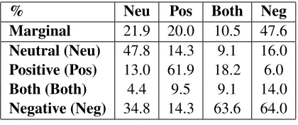
To examine which pair of codings is the most dif-ficult to distinguish, Table 1 summarizes the confu-sion matrix for the three pairs of annotator’s judge-ments on sentiment codings. Each column describes the marginal probability of a coding and the prob-ability distribution for this coding being recognized as another coding (including itself). As many blog-gers use cynical expressions in their writings, the most confusing cases occur when the annotators have to determine whether a snippet is “negative” or “neutral”. The effect of cynical expressions on

% Neu Pos Both Neg

Marginal 21.9 20.0 10.5 47.6

Neutral (Neu) 47.8 14.3 9.1 16.0

Positive (Pos) 13.0 61.9 18.2 6.0

Both (Both) 4.4 9.5 9.1 14.0

Negative (Neg) 34.8 14.3 63.6 64.0

Table 1: Summary matrix for the three on-site annotators’ sentiment codings.

1_{This is done by grouping the codings of Positive, Negative,}

and Both into the subjective class.

sentiment analysis in the political domain is also re-vealed in the second step of alignment annotation. Only 42.5% of the snippets have been coded with alignment coding in the same direction as its senti-ment coding – i.e., if a snippet is intended to support (oppose) a target candidate, it will contain positive (negative) sentiment. The alignment coding task has been shown to be reliable, with the annotators agree-ing 76.8% of the time overall on the three-level cod-ings: Support/Against/Neutral.

2.3.2 Amazon Mechanical Turk Annotation

To compare the annotation reliability between expert and non-expert annotators, we further con-ducted an agreement study with the annotators re-cruited from Amazon Mechanical Turk (AMT). We have collected 1,000 snippets overnight, with the cost of 4 cents per annotation.

In the agreement study, a subset of 100 snippets is used, and each snippet is annotated by five AMT annotators. These annotations were completed by 25 annotators whom were selected based on the ap-proval rate of their previous AMT tasks (over 95% of times).2 _{The AMT annotators spent on average}

40 seconds per snippet, shorter than the average of two minutes reported by the on-site annotators. The lower overall agreement on all four-class sentiment codings, 35.3%, conforms to the expectation that the non-expert annotators are less reliable. The Turk an-notators also agreed less on the three-level alignment codings, achieving only 47.2% of agreement.

However, a finer-grained analysis reveals that they still agree well on some codings: The overall agree-ment on whether a snippet is relevant, whether a snippet is subjective or not, and whether a snippet is positive or negative remain within a reasonable range: 81.0%, 81.8% and 61.9% respectively.

2.4 Gold Standard

We defined the gold standard (GS) label of a snip-pet in terms of the coding that receives the major-ity votes.3 _{Column 1 in Table 2 (onsite-GS}

predic-2_{Note that we do not enforce these snippets to be annotated}

by the same group of annotators. However,Kappastatistics requires to compute the chance agreement of each annotator. Due to the violation of this assumption, we do not measure the intercoder agreement withKappain this agreement study.

3_{In this study, we excluded 6 snippets whose annotations}

onsite-GS prediction onsite agreement AMT-GS prediction AMT agreement

Sentiment (4-class) 0.767 0.704 0.614 0.353

Alignment (3-level) 0.884 0.768 0.669 0.472

Relevant or not 0.889 0.778 0.893 0.810

Subjective or not 0.931 0.861 0.898 0.818

Positive or negative 0.974 0.949 0.714 0.619

Table 2: Average prediction accuracy on gold standard (GS) using one-coder strategy and inter-coder agreement.

tion) shows the ratio of the onsite expert annotations that are consistent with the gold standard, and Col-umn 3 (AMT-GS prediction) shows the same for the AMT annotations. The level of consistency, i.e., the percentage agreement with the gold standard labels, can be viewed as a proxy of the quality of the an-notations. Among the AMT annotations, Columns 2 (onsite agreement) and 4 (AMT agreement) show the pair-wise intercoder agreement in the on-site ex-pert and AMT annotations respectively.

The results suggest that it is possible to take one single expert annotator’s coding as the gold standard in a number of annotation tasks using binary clas-sification. For example, there is a 97.4% chance that one expert’s coding on the polarity of a snip-pet, i.e., whether it is positive or negative, will be consistent with the gold standard coding. However, this one-annotator strategy is less reliable with the introduction of non-expert annotators. Take the task of polarity annotation as an example, the intercoder agreement among the AMT workers goes down to 61.9% and the “one-coder” strategy can only yield 71.4% accuracy. To determine reliable gold stan-dard codings, multiple annotators are still necessary when non-expert annotators are recruited.

3 Annotation Quality Measures

Given the noisy AMT annotations, in this section we discuss some summary statistics that are needed to control the quality of annotations.

3.1 Annotator-level noise

To study the question of whether there exists a group of annotators who tend to yield more noisy annota-tions, we evaluate the accumulated noise level intro-duced by each of the annotators. We define the noise level as the deviation from the gold standard labels. Similar to the measure of individual error rates

pro-posed in (Dawid and Skene, 1979), the noise level of a particular annotatorj, i.e., noise(annoj), is then

estimated by summing up the deviation of the an-notations received from this annotator, with a small sampling correction for chance disagreement. Anal-ysis results demonstrate that there does exist a subset of annotators who yield more noisy annotations than the others. 20% of the annotators (who exceed the noise level 60%) result in annotations that have 70% disagreement with the gold standard.

In addition, we also evaluate how inclusion of noisy annotators reduces the mean agreement with Gold Standard. The plot (left) in Figure 1 plots the mean agreement rate with GS over the subset of an-notators that pass a noise threshold. These results show that the data quality decreases with the inclu-sion of more untrustworthy annotators.

3.2 Snippet-level sentiment ambiguity

We have observed that not all snippets are equally easy to annotate, with some containing more am-biguous expressions. To incorporate this concern in the selection process, a key question to be answered is whether there exist snippets whose sentiment is substantially less distinguishable than the others.

Annotator noise level

Prediction Accuracy

0.0 0.2 0.4 0.6 0.8

0.0

0.2

0.4

0.6

0.8

1.0

Annotator Noise

0.0 0.2 0.4 0.6 0.8 1.0

0.0

0.2

0.4

0.6

0.8

1.0

Sentiment Ambigity

Lexical Uncertainty

Prediction Accuracy

0.0 0.2 0.4 0.6 0.8 1.0

0.0

0.2

0.4

0.6

0.8

1.0

Lexical Uncertainty

Figure 1: Data quality (consistency with GS) as a function of noise level (left), sentiment ambiguity (middle), and lexical uncertainty (right).

be difficult to tell whether they contain negative or neutral sentiment, the measure of example ambigu-ity has to go beyond controversialambigu-ity and incorporate codings of “neutral” and “both”.

To satisfy these constraints, we first enumerated through the codings of each snippet and counted the number of neutral, positive, both, and negative codings: We added (1) one to the positive (nega-tive) category for each positive (nega(nega-tive) coding, (2) 0.5 to the neutral category with each neutral cod-ing, and (3) 0.5 to both the positive and negative categories with each both coding. The strength of codings in the three categories, i.e., str+(snipi),

strneu(snipi), andstr−(snipi), were then summed

up into str(snipi). The distribution were

parame-terized with

θ+(snipi) =str+(snipi)/str(snipi)

θneu(snipi) =strneu(snipi)/str(snipi)

θ₋(snipi) =str−(snipi)/str(snipi)

We then quantify the level of ambiguity in the an-notator’s judgement as follows:

H(θ(snipi)) =−θ+(snipi)log(θ+(snipi))

−θneu(snipi)log(θneu(snipi))

−θ₋(snipi)log(θ−(snipi))

Amb(snipi) =

str(snipi)

strmax ×

H(θ(snipi)),

wherestrmax is the maximum value ofstr among

all the snippets in the collection. The plot (middle) in Figure 1 shows that with the inclusion of snip-pets that are more ambiguous in sentiment disam-biguation, the mean agreement with Gold Standard decreases as expected.

3.3 Combining measures on multiple annotations

Having established the impact of noise and senti-ment ambiguity on annotation quality, we then set out to explore how to integrate them for selection. First, the ambiguity scores for each of the snippets are reweighed with respect to the noise level.

w(snipi) =

X

j

noise(annoj)×(1

e)

θ(ij)

Conf(snipi) =

w(snipi)

P

iw(snipi) ×

Amb(snipi),

where θ(ij) is an indicator function of whether a

coding ofsnipifrom annotatorjagrees with its gold

standard coding. w(expi) is thus computed as the

aggregated noise level of all the annotators who la-beled theith snippet.

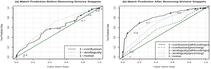
To understand the baseline performance of the se-lection procedure, we evaluate the the true predic-tions versus the false alarms resulting from using each of the quality measures separately to select an-notations for label predictions. In this context, a true prediction occurs when an annotation suggested by our measure as high-quality indeed matches the GS label, and a false alarm occurs when a high quality annotation suggested by our measure does not match the GS label. The ROC (receiver operating charac-teristics) curves in Figure 2 reflect all the potential operating points with the different measures.

0.0 0.2 0.4 0.6 0.8 1.0

0.0

0.2

0.4

0.6

0.8

1.0

False Alarm Rate

True Prediction Rate

● ● ● ● ● ●

●

●

● ●

0.1 0.2 0.3 0.4 0.5

0.6

0.7

0.8

0.9 1

(a) Match Prediction Before Removing Divisive Snippets

1−confusion 1−ambiguity 1−noise

0.0 0.2 0.4 0.6 0.8 1.0

0.0

0.2

0.4

0.6

0.8

1.0

False Alarm Rate

True Prediction Rate

● ● ● ● ● ● ●

●

●

● ●

0 0.1 0.2 0.3 0.4 0.5

0.6

0.7

0.8

0.9

1

(b) Match Prediction After Removing Divisive Snippets

1−confusion(all4codings) 1−confusion(pos/neg) 1−ambiguity(all4codings) 1−ambiguity(pos/neg) 1−noise

Figure 2:Modified ROC curves for quality measures: (a) before removing divisive snippets, (b) after removing divisive snippets. The numbers shown with the ROC curve are the values of the aggregated quality measure (1-confusion).

Initially, three quality measures are tested: 1-noise, 1-ambiguity, 1-confusion. Examination of the snippet-level sentiment codings reveals that some snippets (12%) result in “divisive” codings, i.e., equal number of votes on two codings.

The ROC curves in Figure 2 (a) plot the base-line performance of the different quality measures. Results show that before removing the subset of di-visive snippets, the only effective selection criteria is obtained by monitoring the noise level of anno-tators. Figure 2 (b) plots the performance after re-moving the divisive snippets. In addition, our am-biguity scores are computed under two settings: (1) with only the polar codings (pos/neg), and (2) with all the four codings (all4codings). The ROC curves reveal that analyzing only the polar codings is not sufficient for annotation selection.

The results also demonstrate that confusion, an in-tegrated measure, does perform best. Confusion is just one way of combining these measures. One may chose alternative combinations – the results here pri-marily illustrate the benefit of considering these dif-ferent dimensions in tandem. Moreover, the differ-ence between plot (a) and (b) suggests that removing divisive snippets is essential for the quality measures to work well. How to automatically identify the di-visive snippets is therefore important to the success of the annotation selection process.

3.4 Effect of lexical uncertainty on divisive snippet detection

In search of measures that can help identify the di-visive snippets automatically, we consider the inher-ent lexical uncertainty of an example. Uncertainty Sampling (Lewis and Catlett, 1994) is one common heuristic for the selection of informative instances, which select instances that the current classifier is most uncertain about. Following on these lines we measure the uncertainty on instances, with the as-sumption that the most uncertain snippets are likely to be divisive.

In particular, we applied a lexical sentiment clas-sifier (c.f. Section 4.1.1) to estimate the likelihood of an unseen snippet being of positive or negative sen-timent, i.e., P+(expi), P−(expi), by counting the

sentiment-indicative word occurrences in the snip-pet. As in our dataset the negative snippets far ex-ceed the positive ones, we also take the prior proba-bility into account to avoid class bias. We then mea-sure lexical uncertainty as follows.

Deviation(snipi) =

1

C × |(log(P(+))−log(P(−)))

+(log(P+(snipi))−log(P−(snipi)))|,

U ncertainty(snipi) =1−Deviation(snipi),

where class priors, P(+)and P(₋), are estimated

with the dataset used in the agreement studies, and

Cis the normalization constant.

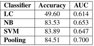
Classifier Accuracy AUC

LC 49.60 0.614

NB 83.53 0.653

SVM 83.89 0.647

Pooling 84.51 0.700

Table 3: Accuracy of sentiment classification methods.

also the utility of such measure in identifying divi-sive snippets. Figure 1 (right) shows the effect of lexical uncertainty on filtering out low-quality anno-tations. Figure 3 demonstrates the effect of lexical uncertainty on divisive snippet detection, suggesting the potential use of lexical uncertainty measures in the selection process.

Lexical Uncertainty

Divisive Snippet Detection Accuracy

0.0 0.2 0.4 0.6 0.8 1.0

0.0

0.2

0.4

0.6

0.8

1.0

Figure 3: Divisive snippet detection accuracy as a func-tion of lexical uncertainty.

4 Empirical Evaluation

The analysis in Sec. 3 raises two important ques-tions: (1) how useful are noisy annotations for sen-timent analysis, and (2) what is the effect of online annotation selection on improving sentiment polar-ity classification?

4.1 Polarity Classifier with Noisy Annotations

To answer the first question raised above, we train classifiers based on the noisy AMT annotations to classify positive and negative snippets. Four dif-ferent types of classifiers are used: SVMs, Naive Bayes (NB), a lexical classifier (LC), and the lexi-cal knowledge-enhanced Pooling Multinomial clas-sifier, described below.

4.1.1 Lexical Classifier

In the absence of any labeled data in a domain, one can build sentiment-classification models that

rely solely on background knowledge, such as a lex-icon defining the polarity of words. Given a lexi-con of positive and negative terms, one straightfor-ward approach to using this information is to mea-sure the frequency of occurrence of these terms in each document. The probability that a test document belongs to the positive class can then be computed asP(+_|D) = _a+a_b; whereaandbare the number

of occurrences of positive and negative terms in the document respectively. A document is then classi-fied as positive ifP(+|D) > P(−|D); otherwise,

the document is classified as negative. For this study, we used a lexicon of 1,267 positive and 1,701 nega-tive terms, as labeled by human experts.

4.1.2 Pooling Multinomials

The Pooling Multinomials classifier was intro-duced by the authors as an approach to incorpo-rate prior lexical knowledge into supervised learn-ing for better text classification. In the context of sentiment analysis, such lexical knowledge is available in terms of the prior sentiment-polarity of words. Pooling Multinomials classifies unlabeled examples just as in multinomial Na¨ıve Bayes clas-sification (McCallum and Nigam, 1998), by predict-ing the class with the maximum likelihood, given by

argmaxcjP(cj)

Q

iP(wi|cj); where P(cj) is the

prior probability of class cj, and P(wi|cj) is the

probability of word wi appearing in a snippet of

classcj. In the absence of background knowledge

about the class distribution, we estimate the class priorsP(cj)solely from the training data. However,

unlike regular Na¨ıve Bayes, the conditional prob-abilities P(wi|cj) are computed using both the

la-beled examples and the lexicon of lala-beled features. Given two models built using labeled examples and labeled features, the multinomial parameters of such models can be aggregated through a convex combi-nation,P(wi|cj) =αPe(wi|cj)+(1−α)Pf(wi|cj);

wherePe(wi|cj)andPf(wi|cj)represent the

proba-bility assigned by using the example labels and fea-ture labels respectively, andαis the weight for

Q1 Q2 Q3 Q4

Accuracy AUC Accuracy AUC Accuracy AUC Accuracy AUC

Noise 84.62% 0.688 74.36% 0.588 74.36% 0.512 79.49% 0.441

Ambiguity 84.21% 0.715 78.95% 0.618 68.42% 0.624 84.21% 0.691

Confusion 82.50% 0.831 82.50% 0.762 80.00% 0.814 80.00% 0.645

Table 4: Effect of annotation selection on classification accuracy.

4.1.3 Results on Polarity Classification

We generated a data set of 504 snippets that had 3 or more labels for either the positive or negative class. We compare the different classification ap-proaches using 10-fold cross-validation and present our results in Table 3. Results show that the Pool-ing Multinomial classifier, which makes predictions based on both the prior lexical knowledge and the training data, can learn the most from the labeled data to classify sentiments of the political blog snip-pets. We observe that despite the significant level of noise and ambiguity in the training data, using majority-labeled data for training still results in clas-sifiers with reasonable accuracy.

4.2 Effect of Annotation Selection

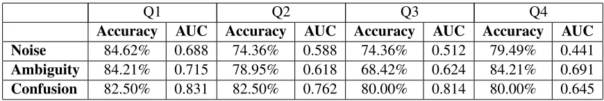
We then evaluate the utility of the quality measures in a randomly split dataset (with 7.5% of the data in the test set). We applied each of the measures to rank the annotation examples and then divide them into 4 equal-sized training sets based on their rankings. For example, Noise-Q1 contains only the least noisy quarter of annotations and Q4 the most noisy ones.

Results in Table 4 demonstrate that the classi-fication performance declines with the decrease of each quality measure in general, despite exceptions in the subset with the highest sentiment ambiguity (Ambiguity-Q4), the most noisy subset Q4 (Noise-Q4), and the subset yielding less overall confusion (Confusion-Q2). The results also reveal the benefits of annotation selection on efficiency: using the sub-set of annotations predicted in the top quality quar-ter achieves similar performance as using the whole training set. These preliminary results suggest that an active learning scheme which considers all three quality measures may indeed be effective in improv-ing label quality and subsequent classification accu-racy.

5 Conclusion

In this paper, we have analyzed the difference be-tween expert and non-expert annotators in terms of annotation quality, and showed that having a single non-expert annotator is detrimental for annotating sentiment in political snippets. However, we con-firmed that using multiple noisy annotations from different non-experts can still be very useful for modeling. This finding is consistent with the sim-ulated results reported in (Sheng et al., 2008). Given the availability of many nexpert annotators on-demand, we studied three important dimensions to consider when acquiring annotations: (1) the noise level of an annotator compared to others, (2) the in-herent ambiguity of an example’s class label, and (3) the informativeness of an example to the current classification model. While the first measure has been studied with annotations obtained from experts (Dawid and Skene, 1979; Clemen and Reilly, 1999), the applicability of their findings on non-expert an-notation selection has not been examined.

References

Giuseppe Carenini and Jackie C. K. Cheung. 2008. Ex-tractive vs. NLG-based absEx-tractive summarization of evaluative text: The effect of corpus controversiality.

InProceedings of the Fifth International Natural

Lan-guage Generation Conference.

R.T. Clemen and T. Reilly. 1999. Correlations and cop-ulas for decision and risk analysis. Management Sci-ence, 45:208–224.

A. P. Dawid and A. .M. Skene. 1979. Maximum likli-hood estimation of observer error-rates using the em algorithm. Applied Statistics, 28(1):20–28.

Jeff Howe. 2008. Crowdsourcing: Why the Power of

the Crowd Is Driving the Future of Business. Crown

Business, 1 edition, August.

Michael Kaisser, Marti Hearst, and John B. Lowe. 2008. Evidence for varying search results summary lengths.

InProceedings of ACL 2008.

Aniket Kittur, Ed H. Chi, and Bongwon Suh. 2008. Crowdsourcing user studies with mechanical turk. In

Proceedings of CHI 2008.

David D. Lewis and Jason Catlett. 1994. Heterogeneous uncertainty sampling for supervised learning. pages 148–156, San Francisco, CA, July.

Andrew McCallum and Kamal Nigam. 1998. A com-parison of event models for naive Bayes text classifi-cation. InAAAI Workshop on Text Categorization. Prem Melville, Wojciech Gryc, and Richard Lawrence.

2009. Sentiment analysis of blogs by combining lexi-cal knowledge with text classification. InKDD. Bo Pang and Lillian Lee. 2004. A sentiment education:

Sentiment analysis using subjectivity summarization based on minimum cuts. InProceedings of ACL 2004. Victor Sheng, Foster Provost, and G. Panagiotis Ipeiro-tis. 2008. Get another label? Improving data quality and data mining using multiple, noisy labelers. In

Pro-ceeding of KDD 2008, pages 614–622.

Vikas Sindhwani and Prem Melville. 2008. Document-word co-regularization for semi-supervised sentiment analysis. InProceedings of IEEE International

Con-ference on Data Mining (ICDM), pages 1025–1030,

Los Alamitos, CA, USA. IEEE Computer Society. R. Snow, B. O’Connor, D. Jurafsky, and A. Ng. 2008.

Cheap and fast—but is it good? evaluating non-expert annotations for natural language tasks. InProceedings

of EMNLP 2008.

Alexander Sorokin and David Forsyth. 2008. Utility data annotation via amazon mechanical turk. InIEEE

Workshop on Internet Vision at CVPR 08.

Qi Su, Dmitry Pavlov, Jyh-Herng Chow, and Wendell C.Baker. 2007. Internet-scale collection of human-reviewed data. InProceedings of WWW 2007.

Peter D. Turney. 2002. Thumbs up or thumbs down: Semantic orientation applied to unsupervised classifi-cation of reviews. InProceedings of ACL 2002. Luis von Ahn and Laura Dabbish. 2004. Labeling

im-ages with a computer game. In Proceedings of CHI 2004, pages 319–326.

Janyce Wiebe and E. Riloff. 2005. Creating subjec-tive and objecsubjec-tive sentence classifiers from unanno-tated texts. InProceedings of CICLing 2005.

Janyce Wiebe, Theresa Wilson, Rebecca Bruce, Matthew Bell, and Melanie Martin. 2004. Learning subjective language.Computational Linguistics, 30 (3).

Jeonghee Yi, Tetsuya Nasukawa, Razvan Bunescu, and Wayne Niblack. 2003. Sentiment analyzer: Extract-ing sentiments about a given topic usExtract-ing natural lan-guage processing technique. In Proceedings of the

International Conference on Data Mining (ICDM),

pages 427–434.