Domain Decomposition of an Optimal Control Problem for Semi Linear Elliptic Equations on Metric Graphs with Application to Gas Networks

(1)

http://www.scirp.org/journal/am

ISSN Online: 2152-7393 ISSN Print: 2152-7385

DOI: 10.4236/am.2017.88082 Aug. 17, 2017 1074 Applied Mathematics

Domain Decomposition of an Optimal Control

Problem for Semi-Linear Elliptic Equations on

Metric Graphs with Application to Gas

Networks

Günter Leugering

Chair of Applied Mathematics II, Friedrich-Alexander-University Erlangen-Nuremberg, Erlangen, Germany Email: [email protected]

Abstract

We consider optimal control problems for the flow of gas in a pipe network. The equations of motions are taken to be represented by a semi-linear model derived from the fully nonlinear isothermal Euler gas equations. We formu-late an optimal control problem on a given network and introduce a time dis-cretization thereof. We then study the well-posedness of the corresponding time-discrete optimal control problem. In order to further reduce the com-plexity, we consider an instantaneous control strategy. The main part of the paper is concerned with a non-overlapping domain decomposition of the semi-linear elliptic optimal control problem on the graph into local problems on a small part of the network, ultimately on a single edge.

Keywords

Optimal Control, Gas Networks, Euler’s Equation, Hierarchy of Models, Semi-Linear Approximation, Non-Overlapping Domain Decomposition

1. Introduction

1.1. Modeling of Gas Flow in a Single Pipe

The Euler equations are given by a system of nonlinear hyperbolic partial differential equations (PDEs) which represent the motion of a compressible non-viscous fluid or a gas. They consist of the continuity equation, the balance of moments and the energy equation. The full set of equations is given by (see [1] [2][3][4]). Let ρ denote the density,

v

the velocity of the gas and p the

pressure. We further denote λ the friction coefficient of the pipe, D the

How to cite this paper: Leugering, G. (2017) Domain Decomposition of an Optim-al Control Problem for Semi-Linear Elliptic Equations on Metric Graphs with Applica-tion to Gas Networks. Applied Mathemat-ics, 8, 1074-1099.

https://doi.org/10.4236/am.2017.88082

Received: June 12, 2017 Accepted: August 14, 2017 Published: August 17, 2017

http://creativecommons.org/licenses/by/4.0/

(2)

DOI: 10.4236/am.2017.88082 1075 Applied Mathematics diameter,

a

the cross section area. The variables of the system are ρ, the flux

q=a vρ . We also denote

c

the the speed of sound, i.e. c2 p

ρ ∂ =

∂ (for constant entropy). For natural gas we have 340 m/s. In particular, in the subsonic case ( v <c), the one which we consider in the sequel, two boundary conditions have to be imposed, one on the left and one on the right end of the pipe. We consider here the isothermal case only. Thus, for horizontal pipes

( )

(

2

)

0

. 2

v t x

v p v v v

t x D

ρ _ρ

λ

ρ ρ ρ

∂ ∂

+ =

∂ ∂

∂ ₊ ∂ ₊ _{= −}

∂ ∂

(1)

In the particular case, where we have a constant speed of sound c p

ρ = _{, for}

small velocities v c, we arrive at the semi-linear model

( )

0

. 2

v t x

p

v v v

t x D

ρ _ρ

λ

ρ ρ

∂ ₊ ∂ ₌

∂ ∂

+ = −

∂ ∂

(2)

1.2. Network Modeling

Let G=

(

V E,

)

denote the graph of the gas network with vertices (nodes)

{

1, 2, , V

}

V = n n  n an edges E=

{

e e1, 2,,eE

}

. Node indices are denoted

,

j∈  =V , while edges are labelled i∈ , = E . For the sake of uniqueness, we associate to each edge a direction. Accordingly, we introduce the edge-node incidence matrix

1, if node is the left node of the edge ,

1, if node is the right node of the edge ,

0, else.

j i

ij j i

n e

d n e

−   = +

 

In contrast to the classical notion of discrete graphs, the graphs considered here are known as metric graphs, in the sense, that the edges are continuous curves. In fact, we consider here straight edges, along which differential equations hold. The pressure variables p ni

( )

j coincide for all edges incident at node

n

j, i.e.

{

}

: 1, , 0

j ij

i∈ = ∈i  E d ≠ . We express the transmission conditions at the

nodes in the following way. We introduce the edge degree d_j:= _j . We

distinguish now between multiple nodes

n

j, where

d

j

>

1

, which we denote M



, whereas for simple nodes

n

j, for which di=1, we write

S



. The set of simple nodes decomposes then into those simple nodes, where Dirichlet conditions hold S

D

 and Neumann nodes S

N

 . Then the continuity conditions read as follows

( )

,

( )

, , , , M,

(

0,

)

.

i j k j j

p n t =p n t ∀i k∈ j∈ t∈ T

(3)

DOI: 10.4236/am.2017.88082 1076 Applied Mathematics

( )

, 0, ,

( )

0, .

j

M

ij i j

i

d q n t j t T

∈

= ∈ ∈

∑

  (4)

From the considerations above we conclude the following system of semi- linear hyperbolic equations on the metric graph G:

( )

( ) (

) (

)

( )

( ) ( )

_{( )}

( ) (

) (

)

( ) ( )

(

)

( )

(

)

( )

(

)

( )

(

)

( )

2

, , 0, , , 0, 0,

, ,

, , , , , 0, 0,

, 2

, , , , , , 0,

, 0, , 0,

, 0

j

i

t i x i i

i

i i

i

t i x i i

i i i

S

j i j i j j j

M

i j k j j

M ij i j

i

i i

c

p x t q x t i x t T

a

q x t q x t c

q x t p x t i x t T

p x t D a

h p n t q n t u t i j t T p n t p n t i k j t T

d q n t j t T

p x p

λ

∈

∂ + ∂ = ∈ ∈ ×

∂ + ∂ = − ∈ ∈ ×

= ∈ ∈ ∈

= ∀ ∈ ∈ ∈

= ∈ ∈

=

∑





 



( ) ( )

( )

(

)

,0 x ,q xi , 0 =qi0 x ,x∈ 0,i ,i∈.

(5)

To the best knowledge of the authors, for problem (5), no published result seems to be available.

2. Optimal Control Problems and Outline

We are now in the position to formulate optimal control problems on the level of (5). There are currently two different approaches towards optimizing and/or control the flow of gas flow through pipe networks. The first one aims at optimizing decision variables such as on-off-states for valves and compressors or zero-full-supply and demand variables for input and exit nodes, respectively. Valves and compressors can be modelled as transmission conditions at a serial node. We refer to [5][6][7] and refrain in the sequel from discussing issues of valves and compressors. The combined discrete and continuous optimization will be the subject of a forthcoming publication. We now describe the general format for an optimal control problem associated with the semi-linear model equations.

( )

(

)

(

)

( )

(

)

( )

2

, ,

0 0 0

min , , : , d d d

2

. . , , satisfies 5 ,

i

S

T T

i i i j

p q u

i j

I p q u I p q x t u t t

s t p q u

ν

∈Ξ _∈

∈

=

∑

_∫∫

 +

∑

_∫

 

(6)

(

)

{

}

: p q u, , :pi pi p qi, i qi q ui, i ui u ii, .

Ξ = ≤ ≤ ≤ ≤ ≤ ≤ ∈

(7)

In (6), ν >0 is a penalty parameter and Ii

( )

⋅ ⋅, a continuous function on

the pairs

( )

p q, . In (7), the quantities p q p qi, ,i i, i are given constants that

determine the feasible pressures and flows in the pipe i, while u u_i, _i describe

control constraints. In the continuous-time case the inequalities are considered as being satisfied for all times and everywhere along the pipes. In the sequel, we will not consider control constraints and state-constraints and, moreover, even reduce to a time semi-discretization.

Time Discretization

(4)

DOI: 10.4236/am.2017.88082 1077 Applied Mathematics break points t0= < <0 t1 <tN =T with widths ∆ =tn: tn+1−t nn, =0,,N−1. Accordingly, we denote p x ti

(

, n

)

=:pi n,

( ) (

x q x t, i , n

)

=:qi n,

( )

x n, =0,,N−1 . We consider a mixed implicit-explicit Euler scheme which takes pi in the friction term in an explicit manner.

( )

(

)

( )

(

)

( )

(

)

( )

2

, 1 , 1 ,

, 1 , 1

2

, 1 , 1

, 2

,

, 1 , 1 , 1

, 1 , 1

, 1

1 1

, 0, , 1

1

, 0, , 2 , , , , , , 0 j i

i n x i n i n i

i

i n x i n

i n i n

i

i n i

i n i i

S

j i n j i n j j n j

M

i n j k n j j

ij i n j

i

c

p x q x p x x i

t a t

q x p x

t

q x q x

c

q x x i

p x t

D a

g p n q n u i j

p n p n i k j

d q n

λ + + + + + + + + + + + + ∈ + ∂ = ∈ ∈ ∆ ∆ + ∂ ∆ = − + ∈ ∈ ∆ = ∈ ∈ = ∀ ∈ ∈ =

∑

        

( )

(

)

,0 ,0 ,0

0

, ,

,

, 0, , .

M

i i i

i i

j

p x p x q x

q x x i

∈ = = ∈ _ ∈   (8)

We then obtain the optimal control problem on the time-discrete level:

( )

(

)

(

)

( )

(

)

( )

2

, , , ,

10 =1

min , , : , d

2

. . , , satisfies 8 .

i

S

N N

i i n i n j

p q u

i n j n

I p q u I p q x u n

s t p q u

ν ∈ = ∈ =

∑∑

_∫

 +

∑ ∑

  (9)

In (9), we consider edgewise given cost functions e.g.

(

)

( )

{

( )

2

( )

2

}

(

)

, , , : , , , , , 0, , .

2

d d

i

i i n i n i n i n i n i n i

I p q x =κ p x −p x + q x −q x x∈  i∈

It is clear that (9) involves all time steps in the cost functional. We would like to reduce the complexity of the problem even further. To this aim we consider what has come to be known as instantaneous control. This amounts to reducing the sums in the cost function of (9) to the time-level tn+1. This strategy has is

known as rolling horizon approach, the simplest case of the moving horizon paradigm, see e.g. [8][9]. Thus, for each n=1,,N−1 and given

p

_{i n}_,

,

q

_{i n}_, , we

consider the problems

( )

(

)

(

)

(

)

( )

2

, ,

0

min , , : , d

2

. . , , satisfies 8 at time level 1.

i

S

i i i j

p q u

i j

I p q u I p q x u

s t p q u n

ν ∈ ∈ = + +

∑



∫

∑

  (10)

It is now convenient to discard the actual time level n+1 and redefine the

states at the former time as input data. To this end, we introduce i: 1

t

α

= ∆ ,

( )

1 , 1 :

i i n

f p x

t = ∆ ,

( )

2 , 1 :

i i n

f q x

t = ∆ ,

( )

2 2 , 1 : 2 i i i n i i c x p x D a λ

(5)

( )

(

)

( )

( ) ( ) ( )

(

)

( ) ( )

(

)

( )

2

1

2

, 0, ,

, , ,

( ), , , 0, .

j

i

i i x i i i

i

i i x i i i i i i

S

j i j i j j j

M

i j k j j

M

ij i j

i

c

p x q x f x i

a

q x p x x q x q x f x i

g p n q n u i j

p n p n i k j

d q n j

α

α γ

∈

+ ∂ = ∈ ∈

+ ∂ + = ∈ ∈

= ∈ ∈

= ∀ ∈ ∈

= ∈

∑





 



(11)

We now differentiate the first equation in (11) with respect to

x

and insert

the result into the second equation. After renaming 2 1 1

:

i i x i

i

f f f

α

= − ∂ _,

{

i 1, ,m

}

= = 

 and introducing

2

i i

c a

β

α

= _{, we consider the semi-linear}

elliptic problem on the graph G with Neumann controls at simple nodes.

( )

(

( )

)

( )

(

)

( )

; , 0, ,

, ,

0, ,

, ,

0, ,

k

i i i xx i i i i i

M

i x i k j x j k k

S

i k k k D

S

x i k k k k N

M ik i k

i

q x q x g x q x f x x i

q n q n i j k

q n i n

q n u i n d q n k

α β

β β

∈

− ∂ + = ∈ ∈

∂ = ∂ ≠ ∈ ∈

= ∈ ∈

∂ = ∈ ∈

= ∈

∑





 



(12)

where we set g x s_i

( )

; :=

γ

_i

( )

x s s . We then consider in the rest of the paper the following optimal control problem:

( )

(

)

(

)

(

)

( )

2 , ,

0

min , , : , d 2 . . , , satisfies 12 .

i

S

i i i j

p q u

i j

I p q u I p q x u

s t p q u

ν

∈ ∈

=

∑



_∫

+

∑

  (13)

Example 1. Before we embark on the non-overlapping domain decomposition method in the context of the instantaneous control paradigm (13), we look into the situation of a star graph with a central multiple node and

m

edges. We

arrange the graph such that the central node is located at x=0 for all right ends of the edges and x=i at the left ends of the edges. This is the situation that we consider in our examples. We assumed that the first edge satisfies a homogeneous Dirichlet condition at x=1 and controlled Neumann conditions

at x=i. We obtain, accordingly

( )

( ) ( ) ( )

( )

(

)

( )

1

( )

1

( )

1

, 0, , 1, ,

0 0 , 1, ,

0 0, 0, 2, , .

i i i xx i i i i i i i

i x i j x j m

i x i i i

i

q x q x x q x q x f x x i m

q q i j m

q q q u i m

α β α γ

β β

=

− ∂ + = ∈ =

∂ = ∂ ≠ =

= = ∂ = =

∑

 



  

(14)

3. Domain Decomposition

(6)

DOI: 10.4236/am.2017.88082 1079 Applied Mathematics monograph [10] for details. The idea for this algorithm originates from a decoupling of the transmission conditions. To this end, we define the flux vector

( )

(

)

T

: ,

k

ik i k k

q = d q n i∈ and the pressure vectors ∂qk:=

(

βi∂x iq n

( )

k ,i∈k

)

T

at a given node , M k

n k∈ . Given a vector z:=

(

z ii, ∈k

)

, we define

( )

(

)

2

: .

k k

j i i

j k

z z z

d ∈

=

∑

−





(15) Then

( )

_k 2

S =I and Sk

( )

1 =1 for 1:=

(

1,,1

)

∈dk. With this notation, the general concept is easily established. We set for any σ>0:

( )

.

k k k k k k

q + ∂ =σ q σ ∂q − q

(16) Applying _k to both sides of (16), we obtain

( )

0.

k

ik i k

i

d q n ∈

=

∑

 (17)

But then (16) reduces to

( )

1

( )

, ,

k

i k j k k

k k

q n q n i

d ∈

∂ =

∑

∂ ∈

 

which, in turn, implies

( )

, , M.

i x iq nk j xq nj k i j k k

β

∂ = ∂

β

≠ ∈ ∈ ₍₁₈₎

Clearly, if the transmission conditions (17), (18) hold at the multiple node nk, then (16) is also fulfilled. Thus, (16) is equivalent to the transmission conditions (17), (18). These new conditions (16) are now relaxed in an iterative scheme as follows. We use l as iteration number.

( )

1

( )

1

( )

1

: .

l l l l l

k k k k k k k

p + + ∂σ q + =σ ∂q − q = g +

(19) We have the following relations:

( )

1

(

( ) ( )

)

2 .

l l l

k k k k

g + = σ∂ q − g

(20) This gives rise to the definition of a fixed point mapping. To this end, we need to look into the behavior of the interface in terms of k, M

g k∈ , that is

2 2

,

1

: M _k, : ,

M k

i i k

k

i k

g g g

σ

∈ ∈

∈ = Π Π _ _ =

∑ ∑



 



(21)

: → ,

   ₍₂₂₎

( )

g i k_, :=k

(

2σ∂

( )

qk −gk

)

_i,k∈M,i∈k,

( )

g k=

{

( )

 i k, ,i∈k

}

,

( )

{

_k, M

}

.

g= g k∈

  

Now,

( )

(

)

2

2 1

2 .

M k

k k k

i i

k

g µ q g

σ

∈ ∈

=

∑ ∑

∂ −



 

 

(23) We use the facts _k

(

k k

)

2 _k

( )

k 2

i∈

g

_i

=

i∈

g

_i

(7)

(

) (

)

k k

k k k k k k

i i

i∈ q i g i= i∈ q g

∑

  

∑

 and show

(

)

2 2

4 .

M k

k k k

i i i

i k

g g g σ q q

∈ ∈ = −

∑ ∑

− ∂ ∂      (24) We now formulate a relaxed version of a fixed point iteration: for ∈

[ )

0,1

(

)

( )

1

1 .

l l l

g+ = −  g +g

(25) Up to now, the relations concerning the iteration at the interfaces do not involve the state equation explicitly. For the analysis of the convergence of the iterates, we need to specify the equations.

The Non-Overlapping Domain Decomposition

We are interested in the errors between the solutions to the problem (12) and

( )

(

)

( )

1 1 1

1 1

1

, 0, , 0, ,

, ,

2 2

, .

l l l

i i i xx i i i i i

S

i k k k D

S

x i k k k k N

l l

ik i k x i k

l l l l

j x j k i x i k ik j k ik i k

j j

k k k k

l M

ik

q x q x g q f x x i

q n i n

q n u i n

d q n q n

q n q n d q n d q n

d d

g k

α β

σ

σ β β

+ + + + + ∈ ∈ + − ∂ + = ∈ ∈ = ∈ ∈ ∂ = ∈ ∈ + ∂     = _ ∂ − ∂  _{ }− − _     = ∈

∑

         (26)

Thus, we introduce 1 1

:

l l

e+ =q+ −q. Then el+1 solves a non-linear differential

equation with nonlinearity

(

l 1

)

( )

i i i i i

g e+ +q −g q , zero right hand side and

homogeneous boundary conditions at the simple nodes. As we noted above, the full transmission conditions are equivalent to (16). Hence, the error satisfies the same iterative Robin-type boundary conditions as l1

q+ . We consider the following integration by parts formula after multiplying by a test function φ_.

(

)

(

1 1 1

)

0

0 ( ) d

i

l l l

i i i xx i i i i i i i

i

e e g e q g q x

α + β + + φ

∈

=

∑∫

 − ∂ + + −

 (27)

( ) ( )

1

M k

l

ik i x i k i k i

k

d β e+ n φ n

∈ ∈ = −

∑ ∑

∂   (28)

(

)

( )

(

)

(

1 1 1

)

0

d .

i

l l l

i i i i x i x i i i i i i i

i

e e g e q g q x

α +φ β + φ + φ

∈

+

∑∫

 + ∂ ∂ + + −

 (29)

We now take the test function to be equal to l 1

i

e+ and obtain:

( ) ( )

(

)

( )

(

)

(

)

1 1

1 1 1 1 1 1

0 d . M k i l l

ik x i k i k

i k

l l l l l l

i i i i x i x i i i i i i i

i

d e n e n

e e e e g e q g q e x

α β + + ∈ ∈ + + + + + + ∈ ∂ = + ∂ ∂ + + −

∑ ∑

∑∫

    (30)

We use the boundary condition at the interfaces in the form

( )

1 1 1

, .

l l l M

ik i k ik x i k

d e+ n =g+ − ∂

σ

e+ n k∈

(8)

(

)

2 2

4 .

M k

k k k

i i i

i k

g g g σ e e

∈ ∈

= −

∑ ∑

− ∂ ∂

 

 



(31) We obtain

(

)

( )

(

)

(

)

2 2

1

2

0

4 d .

i

l l

l l l l l l l

i i i i x i x i i i i i i i i

g g

g αe e β e e g e q g q e x

+

∈

=

= −

∑∫

 + ∂ ∂ + + −

 

 _



(32) We assume

( )

(

g_i x s; −g_i x t;

)

(

s− ≥ ∀ ∈t

)

0, x

(

0,_i

)

,i∈

(33) and define the bilinear form

(

)

(

)

0

, : d .

i

i i i i i i x i x i

a ψ φ =

∫

αψ φ β ψ φ+ ∂ ∂ x 

(34) We define the corresponding quadratic form applied to l

e

( ) (

)

0

, : d ,

i

l l l l l l

i i i i i i i x i x i

a e e =

∫

αe e + ∂ ∂β e e x 

(35) which is certainly bounded below by 2( )_0,

i

i L

e _ . Then the error iteration is

(

)

2 2 2

1

4 ,

l l l l l

i i i

i

g+ g g a e e

∈

= = −

∑

    _

(36) and, thus, the error does not increase. That it actually decreases to zero is shown next. But first we look at the relaxed version of the iteration (25). We take norms and calculate in order to obtain (for ∈

[ ]

0,1

(

)

(

)

2 2

1

4 1 , .

l l l l

i i i

i

g+ g a e e

∈

≤ − −

∑

   _

(37) We iterate in (36) or (37) down from l to zero. Then we obtain

{ }

l is bounded,

(

l, l

)

0, . i i i

g a e e → l→ ∞

(38) Clearly, for α_i>0, this shows that the H1

(

0,i

)

-error strongly tends to zero.

Then also the traces tend to zero as l→ ∞ and, therefore, the iteration converges.

Theorem 2. Under assumption (33), for each ∈

[ )

0,1 the iteration (25)

with (26) and (21), (22) converges as l→ ∞. The convergence of the solutions is in the sense of (38).

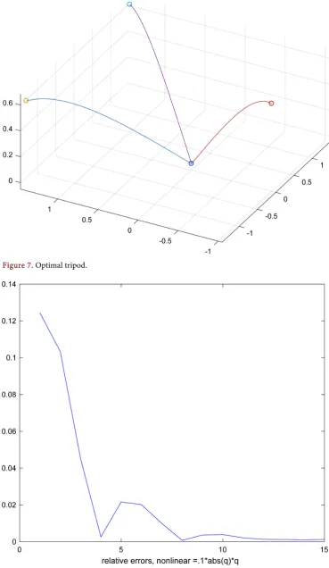
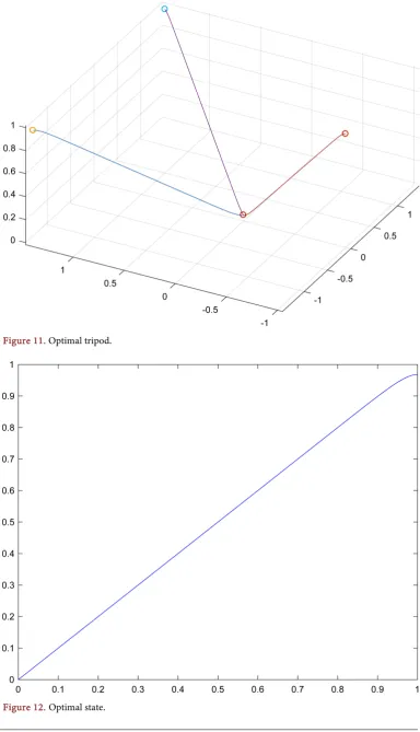
Example 3. We show a numerical example, where three edges span a tripod. The first edge (see Figure 1) satisfies homogeneous Dirichlet conditions at the exterior node, while for the other two edges satisfy homogeneous Neumann conditions at the exterior nodes. In particular, we take dx=1 1000, αi=10,

1 1

f = , f₂=0.1, f₃=0.5. The nonlinearity is weighted by a factor γ=1 and

there are 10 fixed point iterations in order to handle the nonlinearity. The system without domain decomposition is solved using the MATLAB routine bvp4c with error tolerance tol= −1e 10. The system with domain decomposition

(9)

[image:9.595.213.535.188.425.2]

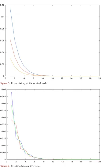
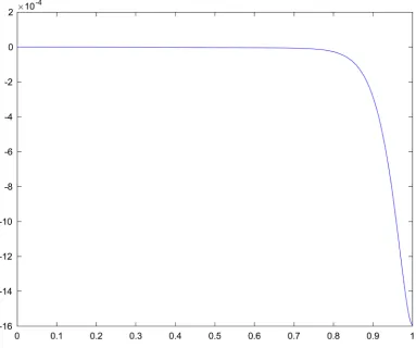
DOI: 10.4236/am.2017.88082 1082 Applied Mathematics domain decomposition. No difference is visible. Notice the discontinuity of the state at the central node. This is contrast to the classical nodal conditions known in the literature, where the states are continous across the multiple node, while the Neumann traces satisfying the Kirchhoff condition. We display the individual solutions—again without and with domain decomposition in Figure 2. There is no visible difference. Figure 3 shows the nodal errors at the central node. We see the nodal errors regarding the conservation of flows and the two

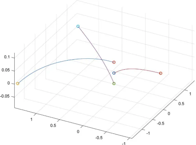
Figure 1. The tripod with disciniuity at the central node.

[image:9.595.213.536.437.733.2]

(10)

[image:10.595.208.540.58.604.2]

Figure 3. Error history at the central node.

Figure 4. Iteration history L∞_-errors.

continuity conditions of the derivatives at the central node. In Figure 4, we display the relative L∞-errors of the solutions, where the errors are taken with

respect to the computed solution without domain decomposition.

(11)

DOI: 10.4236/am.2017.88082 1084 Applied Mathematics ( )

( )

(

( )

)

( )

(

)

( )

2 2 0 ,

min , :

2 2

subject to

; , 0, ,

0, , , , , , , 0, . S N k

i i k

q u _i

k

i i i xx i i i i i

S

i k k k D

S

x i k k k k N

M

i x i k j x j k k

M ik i k

i

I q u q q u

q x q x g x q x f x x i

q n i n

q n u i n

q n q n i j k

d q n k

κ ν α β β β ∈ ∈ ∈ = − + − ∂ + = ∈ ∈ = ∈ ∈ ∂ = ∈ ∈ ∂ = ∂ ≠ ∈ ∈ = ∈

∑

            (39)

The corresponding optimality system then reads as follows:

( )

(

)

( )

(

)

(

)

( )

0

in 0, ,

in 0, , 0, 0, ,

1

, 0, ,

, , ,

0

k k

i i i xx i i i i i

i i i xx i i i i i i i

S

i k i k k k D

S

x i k i k x i k k k N

M

i x i k j x j k i x i k j x j k k

ik i k ik i

i i

q q g q f i

g q q q i

q n n i n

q n n n i n

q n q n n n i j k

d q n d

α β

α ρ β ρ ρ κ

ρ

ρ ρ

ν

β β β ρ β ρ

ρ ∈ ∈ − ∂ + = ∈ ′ − ∂ + = − − ∈ = = ∈ ∈ ∂ = ∂ = ∈ ∈ ∂ = ∂ ∂ = ∂ ≠ ∈ ∈ = =

∑

           

( )

, M.

k

n k∈

(40)

The idea now is to use a domain decomposition similar to the original system on the network. We design a method that allows to interpret the decomposed optimality system (41) as an edge-wise optimality system of an optimal control problem formulated on an individual edge. To this end, we introduce the following local system:

(

)

(

)

(

)

( )

1 1

1 1 1 0

1 1

1 1 1

in 0, ,

0, 0, ,

1

, 0, ,

2

k

l l

i i i xx i i i

l l l

i i i xx i i i i

l l S

i k i k k k D

l l l S

x i k i k x i k k k N

l l l

ik i k k x i k k x i k

l

k j x k k

j k

q q f i

q q i

q n n i n

q n n n i n

d q n q n n

q n d

α β

α ρ β ρ κ

ρ

ρ ρ

ν

λ µ ρ

λ β + + + + + + + + + + + + + ∈ − ∂ = ∈ − ∂ = − − ∈ = = ∈ ∈ ∂ = ∂ = ∈ ∈ + ∂ + ∂ =

∑

∂ −         

( )

1

1 1 1

2 2 , 2 2 2 k k k k

l l l

i x i k k j x k k i x i k

j k

l l l

ik j k ik i k ik

j k

l l l

ik i k k x i k k x i k

l l l l

k j x k k i x i k k j x j k i x i k

j j

k k

q n n n

d

d q n d q n g

d

d n n q n

n n q n q n

d d

d

β µ β ρ β ρ

ρ λ ρ µ

λ β ρ β ρ µ β β

∈ + ∈ + + + ∈ ∈     ∂ + ∂ − ∂           − − =   + ∂ − ∂     =  ∂ − ∂ −  ∂ − ∂      −

∑

   

( )

1

, .

k

l l l M

ik k k ik i k ik

j k

d ρ n d ρ n h+ k

∈   − = ∈   

∑

   (41)

(12)

DOI: 10.4236/am.2017.88082 1085 Applied Mathematics upon convergence as l→ ∞, the system (41) tends to (40). Now, (41) decomposes the fully connected problem (40) to a problem on a single edge

i∈ with inhomogeneous Robin-type boundary conditions. The question is as

to whether the decomposed optimality system (41) is in fact itself an optimality system on that edge. If so, then it is possible to parallelize the optimization problems rather than the forward and backward solves. Let us, therefore, now consider the following optimization problems on a single edge. The idea is to introduce a virtual control that aims at controlling classical inhomogeneous Neumann condition including the iteration history at the interface as inhomogeneity to the Robin-type condition that appears in the decomposition. To this end, it is sufficient to consider three cases: a.) the edge i connects a controlled

Neumann S

N

j∈ node with a multiple node

k

∈



M at which the domain

decomposition is active, b.) the edge i connects a controlled Neumann node S

N

j∈ with multiple node

k

∈



M at which the domain decomposition is

active, c.) the edge i connects two multiple nodes j k, ∈M.

Case a.):

(

)

(

( )

)

( )

(

)

( )

2 2

0 2 2

,

1 1

min , , :=

2 2 2 2

subject to

, 0,

, .

j ik

l

i j ik i i j ik k x i k ik

u v

k k

i i i xx i i i i i

l

ik i j j ik i k k i x i k ik ik

I q u v q q u v q n h

q q g q f x

d q n u d q n q n g v

κ ν _µ

µ µ

α β

λ β

− + + + ∂ +

− ∂ + = ∈

= = − ∂ + +



(42)

Case b.):

(

)

(

( )

)

( )

(

)

( )

2 2

0 2 2

,

1 1

min , , :

2 2 2 2

subject to

, 0,

, .

j ik

l

i i i i i i ik k i x i k ik

u v

k k

i i i xx i i i i i

l

ij i x i j j ik i k k x i k ik ik

I q u v q q u v q n h

q q g q f x

d q n u d q n q n g v

κ ν _{µ β}

µ µ

α β

β λ

= − + + + ∂ +

− ∂ + = ∈

∂ = = − ∂ + +



(43)

Case c.):

(

)

( )

(

)

(

( )

)

( )

(

)

( )

2

0 2 2

,

2 2

1 1

min , , :

2 2 2

1 1

2 2

subject to

, 0,

, .

ij ik

i ij ik i i ij ik

v v

j k

l l

k i x i k ik j i x i j ij

k j

i i i xx i i i i i

l l

ij i j j i x i j ij ij ik i k k i x i k ik ik

I q v v q q v v

q n h q n h

q q g q f x

d q n q n g v d q n q n g v

κ

µ µ

µ β µ β

µ µ

α β

λ β λ β

= − + +

+ ∂ + + ∂ +

− ∂ + = ∈

= − ∂ + + = − ∂ + +



(44)

Remark 4.1.

• _{If we write down the optimality systems for (42), (43) and (44), respectively,} and combine the results, we arrive at (41).

(13)

DOI: 10.4236/am.2017.88082 1086 Applied Mathematics with input data coming from the iteration history that involves all nodes adjacent at the ends of the given edge.

• _{This means that we can actually decompose the optimization problem given} on the graph into a sequence of local optimization problems given on an individual edge.

• _{The resulting optimization problem on the individual edges are strictly} convex, thus, admitting a unique global solution.

Remark 4.2. There are at least two ways to use the proposed ddm-approach. 1) In the first approach, we consider (40) and start with a guess for the adjoint variables

( )

ρ

i i∈. This provides a guess for the controls

( )

uj _j_∈_S. Therefore, we can establish the states

( )

qi i∈. The states

( )

qi i∈, in turn, are inserted into the

adjoint problem and that system is then solved for

( )

ρ

i i∈, which closes the

cycle. With this method, we keep the optimization in an outer loop and solve both the forward system for the states

( )

qi i∈ and the adjoint system for

( )

ρ

_{i i}_∈__{, individually. For given}

( )

q_{i i}_∈_, the adjoint system is a linear elliptic problem on the graph. To this system the ddm-method above applies and converges. As we have established above, the forward problem admits a convergent ddm-algorithm. This finally means that in the inner loop we can use convergent ddm-iterations for finding

( )

qi i∈ and

( )

ρ

i i∈ . The effect of

parallelization can, therefore, be used for the solves in the inner loop, while the outer loop is sequential.

2) In the second approach, we decompose the coupled system (40) to (41). The resulting decoupled problem is then the optimality system for the virtual optimal control problems (42), (43) or (44), as seen above. In this case, there is no outer loop other than the ddm-iteration which is completely parallel. Still, the local optimality systems have to be solved in a way describes in the first approach. Namely, we provide an initial guess for ρi for each i∈ then solve for qi which is introduced then in the local adjoint equations. This is then followed by the solve for ρi and the update of the boundary data gik,hik which are used in the communication at the next ddm-iteration. In this, admittedly, more elegant approach, the constrained minimization problem on the entire graph can be decomposed to minimization problems on a single edge. As we will see below, unfortunately, but expectedly, the convergence is no longer global as in the first approach, but rather local. This means that only if we start close to a solution of (40), or if we have a priori estimates and tune the parameters accordingly, we can prove convergence of the unique solutions of (41) to those of (40).

5. Wellposedness

5.1. Wellposedness of the Primal Problem

(14)

(

)

1

0, _i .

i∈ H

=

∏

_ _



Indeed, we also define the energy space

( )

: 0, , , 0,

k

S M

i k k k D ik i k

i

q q n i n d q n k

∈

 

 

=_ ∈ = ∈ ∈ = ∈ _

 



∑

 

    

and the operator  as follows:

( )

: i i i xx i in

q =

α

q x − ∂

β

q x

 

( )

{

( )

}

: , , ,

0, , .

M

i x i k j x j k k

S

x i k k k N

D q q n q n i j k

q n i n

β β

= ∈ ∂ = ∂ ≠ ∈ ∈

∂ = ∈ ∈

   

 

(45)

It is a matter of applying standard integration by parts to show that, indeed,  is symmetric and positive definite in  such that  can be extended as a self-adjoint operator in . Then it is standard to show that  can be extended to a bounded coercive map from  into its dual _*. If we assume

(33) and define the Nemitskji operator 

( )( )

q x :=g q x

(

( )

)

then  is strictly

monotone and continuous. Hence, according to [11],  + is strictly monotone and continuous and, hence, the semi-linear problem admits a unique solution q∈. Clearly, for regular right hand sides f , the solution is in

( )

D  .

5.2. Smoothness of the Control-to-State-Map

Let q uˆ_t

( )

ˆ be the solution of (12) with

u

replaced with u tu+ ˆ and let q be

the solution of (12). We denote by e:= −qˆ q the difference of these solutions.

We obtain

( )

(

)( )

( )( )

(

)

( )

0, 0, ,

, ,

0, , ˆ , ,

0, .

k

M

i x i k j x j k k

S

i k k k D

S

x i k k k k N

M

ik i k

i

e x e x g e q x g q x x i

e n e n i j k

e n i n

e n tu i n

d e n k

α β

β β

∈

− ∂ + + − = ∈ ∈

∂ = ∂ ≠ ∈ ∈

= ∈ ∈

∂ = ∈ ∈

= ∈

∑





 



(46)

Dividing by t and letting t tend to zero in (12) implies with

( )( )

ˆ

( )( )

ˆ

:

e′=e u u′ =

δ

e u u

( )

( )( ) ( )

(

)

( )

0, 0, ,

, ,

0, , ˆ , ,

0, .

k

i i i xx i i i i i

M

i x i k j x j k k

S

i k k k D

S

x i k k k k N

M

ik i k

i

e x e x g q x e x x i

e n e n i j k

e n i n

e n u i n

d e n k

α β

β β

∈

′ − ∂ ′ + ′ ′ = ∈ ∈

′ ′

∂ = ∂ ≠ ∈ ∈

′ = ∈ ∈

′

∂ = ∈ ∈

′ = ∈

∑





 



(47)

For the solution q of (12), applying the standard Lax-Milgram Lemma, e′

(15)

DOI: 10.4236/am.2017.88082 1088 Applied Mathematics the classical Weierstrass theorem, problem (39) admits a unique solution. One can then verify the conditions for the Ioffe-Tichomirov Theorem [12] in order to establish the first order optimality conditions (40).

Theorem 4. Under the assumption (33), for *

f∈ , there exists a unique solution q∈ of (12). In addition, the mapping from

u

into q is Gateaux

differentiable. Moreover, the optimal control problem (39) admits a unique solution. The optimal solution is characterized by the optimality system of first order (40).

5.3. A Priori Error Estimates for the Optimality System

We denote the errors l: l

i i i

e = −q q and l: l

i i i

p =

ρ

−

ρ

for i∈ and l=0,1,.

These errors solve the system equations:

(

)

( )

(

)

(

)

(

)

( )

)

(

)

( )

1 1 1

1 1 1 1 1

1

1 1

1 1 1

0, in 0, ,

in 0, ,

0, 0, ,

1

, 0, ,

l l l

l l l l l

i i i xx i i i i i i i i i i i

l

i i

l l S

i k i k k k D

l l l S

x i k i k x i k k k N

l ik i

e e g e q g q i

p p g e q p g e q g q

e i

e n p n i n

e n p n p n i n

d e

α β

α β ρ

κ ν + + + + + + + + + + + + + + − ∂ + + − = ∈ ′ ′ ′ − ∂ + + + + − = − ∈ = = ∈ ∈ ∂ = ∂ = ∈ ∈        

( )

1 1 1

1

1 1 1

2 2 2 , 2 k k k k l l

k k x i k k x i k

l l l l

k j x k k i x i k k j x k k i x i k

j j

k k

l l l

ik j k ik i k ik

j k

l l l

ik i k k x i k k x i k

l

k j x k k i x

j k

n e n p n

e n e n p n p n

d d

d e n d e n g

d

d p n p n e n

p n p

d

λ µ

λ β β µ β β

λ µ

λ β β

+ + + ∈ ∈ + ∈ + + + ∈ + ∂ + ∂     =  ∂ − ∂ +  ∂ − ∂        − − =   + ∂ − ∂ = ∂ − ∂

∑

   

( )

1

2 2

, .

k

l l l

i k k j x j k i x i k

j k

l l l M

ik k k ik i k ik

j k

n e n e n

d

d p n d p n h k

d

µ β β

∈ + ∈     − ∂ − ∂           −_ − _= ∈  

∑

   (48)

We prove the following

Lemma 5. The solutions e p_i, _i for i∈ of (48) satisfies the estimate

( ) ( )

(

( )

)

{

}

1 1

2 2

2 2 2 2 2 2

0,i 0,i

0

0 .

i H i H i i i i i i ij ij

e

_

+

p

_

+

γ

e

+

e



+

p

+

p



≤

C g

+

h

(49)

More precisely, for

λ

k = ∀ ∈

λ

, k M , we obtain

( )

(

)

2

{

}

2 2 2 2

1

4

.

i i i i ij ij

i

e p ν g h

λ =

+ ≤

∑

+

 

(50) Remark 5.1. As a result, for small data

g h

_ij

,

_ij, we have small solutions. Proof of Lemma 5: We multiply the equations in (48) by l1

i

e+ and pil1

(16)

5.4. Convergence

(

)

₂

(

)

2

(

2 2

)

, ,

, : M , , : ,

k _M

k

i k i k

k i

i k

g h _∈ _∈ g h g h

∈ ∈ ∈ =

∏

_

∏

_ _ _ =

∑ ∑

+    (51) : → ,

   ₍₅₂₎

(

)

(

( )

)

( )

(

)

(

)

,

, : 2 ,

2 , , ,

k k k k

k x k x

i k _i

k k k k M

k x k x k

i

g h e p g

p e h k i

λ µ λ µ = ∂ + ∂ − ∂ − ∂ − ∈ ∈     

(

g h,

)

k =

{

( )(

g h,

)

i k, ,i∈ k

}

,

  

(

g h,

)

=

{

(

g h,

)

_k,k∈ M

}

.

   Now,

(

)

(

( )

)

( )

(

)

(

)

( )

(

( )

)

(

)

( )

(

( )

)

(

)

2 2 2 2 2 , 2 2 4 4 . M M M

k k k k

k x k x

ik i

k

k k k k

k x k x

ik

ik ik i k i k x i k k x i k

i k

ik ik i k i k x i k k x i k

i k

g h e p g

p e h

g d e n e n p n

h d p n p n e n

λ µ

β λ µ

∈ ∈ ∈ ∈ ∈ ∈ = ∂ + ∂ − + ∂ − ∂ − = − ∂ + ∂ + − ∂ − ∂

∑ ∑

          (53)

We multiply the state equation for the errors ei, pi by ei and pi, respectively.

(

)

( )

(

)

( ) ( )

( )

(

)

(

)

( )

)

{

}

0 2 2 0 0 d d , i k i

i i i xx i i i i i i i i

ik i x i k i k k i

i i i x i i i i i i i

i

e e g e q g q e x

d e n e n

e e g e q g q e x

α β β α β ∈ ∈ ∈ ∈ = − ∂ + + − = − ∂ + + ∂ + + −

∑∫

∑ ∑

∑∫

      (54)

(

)

(

)

( )

)

(

)

( ) ( )

{

( )

(

)

(

)

(

)

( )

)

}

0 2 2 0 2 0 d d . i i k

i i i xx i i i i i i i i i i i i i i

i

ik i x i k i k i i i x i

k i i

i i i i i i i i i i i i i i

p p g e q p g e q g q e p x

d p n p n p p

g e q p g e q g q p e p x

α β ρ κ

β α β

ρ κ ∈ ∈ ∈ ∈ ′ ′ ′ = − ∂ + + + + − + = − ∂ + + ∂ ′ ′ ′ + + + + − +