Proceedings of the NAACL HLT 2010 Workshop on Semantic Search, pages 27–35,
A Graph-Based Semi-Supervised Learning for Question Semantic Labeling
Asli Celikyilmaz Computer Science Division University of California, Berkeley
Dilek Hakkani-Tur
International Computer Science Institute Berkeley, CA
Abstract
We investigate a graph-based semi-supervised learning approach for labeling semantic com-ponents of questions such as topic, focus, event, etc., for question understanding task. We focus on graph construction to handle learning with dense/sparse graphs and present
Relaxed Linear Neighborhoods method, in which each node is linearly constructed from varying sizes of its neighbors based on the density/sparsity of its surrounding. With the new graph representation, we show perfor-mance improvements on syntactic and real datasets, primarily due to the use of unlabeled data and relaxed graph construction.
1 Introduction
One of the important steps in Question Answering (QA) isquestion understandingto identify semantic components of questions. In this paper, we inves-tigate question understanding based on a machine learning approach to discover semantic components (Table 1).
An important issue in information extraction from text is that one often deals with insufficient la-beled data and large number of unlala-beled data, which have led to improvements in semi-supervised learning (SSL) methods, e.g., (Belkin and Niyogi., 2002b), (Zhou et al., 2004). Recently, graph based SSL methods have gained interest (Alexandrescu and Kirchhoff, 2007), (Goldberg and Zhu, 2009). These methods create graphs whose vertices corre-spond to labeled and unlabeled data, while the edge weights encode the similarity between each pair of data points. Classification is performed using these graphs by scoring unlabeled points in such a way
W hat | {z }
other
f ilm | {z }
f ocus
introduced | {z }
event
J ar J ar Binks
| {z }
topic
?
Semantic Components & Named-Entitiy Types topic:’Jar’ (Begin-Topic); ’Jar’ (In-Topic) ;
’Binks’ (In-Topic)(HUMAN:Individual)
focus:’film’ (Begin-Focus) (DESCRIPTION:Definition)
action / event:’introduced’ (Begin-Event)
expected answer-type:ENTITY:creative
Table 1: Question Analysis - Semantic Components of a sample question from TREC QA task.
that instances connected by large weights are given similar labels. Such methods can perform well when no parametric information about distribution of data is available and when data is characterized by an un-derlying manifold structure.
graphs, yielding disconnected components or sub-graphs or isolated singleton vertices. We propose a Relaxed Linear Neighborhood (RLN) method to overcome fixed k or assumptions. RLN approx-imates the entire graph by a series of overlapped linear neighborhood patches, where neighborhood N(xi)of any nodexiis captured dynamically based on the density/sparsity of its surrounding. Moreover, RLN exploits degree of neighborhood during re-construction method rather than fixed assignments, which does not get affected by outliers, producing a more robust graph, demonstrated in Experiment #1. We present our question semantic component model in section 3 with the following contributions: (1) a new graph construction method for SSL, which relaxes neighborhood assumptions yielding robust graphs as defined in section 5,
(2) a new inference approach to enable learning from unlabeled data as defined in section 6.
The experiments in section 7 yield performance im-provement in comparison to other labeling methods on different datasets. Finally we draw conclusions.
2 Related Work on Question Analysis
An important step in question analysis is extracting semantic components likeanswer type, focus, event, etc. The ’answer-type’ is a quantity that a question is seeking. A question’topic’usually represents ma-jor context/constraint of a question (”Jar Jar Binks” in Table 1). A question’focus’(e.g., film) denotes a certain aspect (or descriptive feature) of a question ’topic’. To extract topic-focus from questions, (Ha-jicova et al., 1993) used rule-based approaches via dependency parser structures. (Burger, 2006) im-plemented parsers and a mixture of rule-based and learning methods to extract different salient features such as question type, event, entities, etc. (Chai and Jin, 2004) explored semantic units based on their discourse relations via rule-based systems.
In (Duan et al., 2008) a language model is pre-sented to extract semantic components from ques-tions. Similarly, (Fan et al., 2008)’s semantic chunk annotation uses conditional random fields (CRF) (Lafferty et al., 2001) to annotate semantic chunks of questions in Chinese. Our work aparts from these studies in that we use a graph-based SSL method to extract semantic components from
unla-beled questions. Graph-based methods are suitable for labeling tasks because when two lexical units in different questions are close in the intrinsic ge-ometry of question forms, their semantic compo-nents (labels) will be similar to each other. Labels vary smoothly along the geodesics, i.e., manifold assumption, which plays an essential role in SSL (Belkin et al., 2006).
This paper presents a new graph construction to improve performance of an important module of QA when labeled data is sparse. We compare our re-sults with other graph construction methods. Next, we present the dataset construction for our semantic component labeling model before we introduce the new graph construction and inference for SSL.
3 Semantic Component Labeling
Each word (token) in a question is associated with a label among a pre-determined list of semantic tags. A questioni is defined as a sequence of in-put units (words/tokens)xi = (x1i, ..., xT i) ∈ XT which are tagged with a sequence of class labels, yi = (y1i, ..., yT i) ∈ YT, semantic components. The task is to learn classifier F that, given a new sequencexnew, predicts a sequence of class labels ynew = F(xnew). Among different semantic com-ponent types presented in previous studies, we give each token a MUC style semantic label from a list of 11 labels.
(1) O:other;
(2) BT:begin-topic;
(3) IT:in-topic
(4) BF:begin-focus;
(5) IF:in-focus
(6) BE:begin-event;
(7) IE:in-event
(8) BCL:begin-clause
(9) ICL:in-clause
(10) BC:begin-complement
(11) IC:in-complement
More labels can be appended if necessary. The first token of a component gets ’begin’prefix and con-secutive words are given’in’prefix, e.g.,Jar (begin-topic), Jar (in-(begin-topic), Binks (in-topic)in Table 1.
rep-resents a relation betweenxi andxj. The task is to assign a label (out of 11 possible labels) to each to-ken of a question i, xti,t = 1, ..., T, T is the max number of tokens in a given query. We introduce a set of nodes for each token (xti), each represent-ing a binary relation between that token and one of possible tags (yti). A binary relation represents an agreement between a given token and assigned label, so our SSL classifier predicts the probability of true relation between token and assigned label. Thus, for each token, we introduce 11 different nodes us-ing yk ∈ {O,BT,IT,BF,IF,BC,IC,BE,IE,BCL,ICL}. There will be 11 label probability assignments ob-tained from each of the 11 corresponding nodes. For labeled questions, intuitively, only one node per ken is introduced to the graph for known(true) to-ken/label relations. We find the best question label sequence via Viterbi algorithm (Forney, 1973).
3.1 Feature Extraction For Labeling Task
The following pre-processing modules are built for feature extraction prior to graph construction.
3.1.1 Pre-Processing For Feature Extraction
Phrase Analysis(PA):Using basic syntactic anal-ysis (shallow parsing), the PA module re-builds phrases from linguistic structures such as noun-phrases (NN), basic prepositional noun-phrases (PP) or verb groups (VG). Using Stanford dependency parser (Klein and Manning, 2003), (Marneffe et al., 2006), which produces 48 different grammatical re-lations, PA module re-constructs the phrases. For example for the question in Table 1, dependency parser generates two relations:
−nn(Binks-3, Jar-1)andnn(Binks-3, Jar-2), PA reveals ”Jar Jar Binks” as a noun phrase re-constructing the nn:noun compound modifier. We also extract part of speech tags of questions via de-pendency parser to be used for feature extraction.
Question Dependency Relations (QDR):Using shallow semantics, we decode underlying Stanford dependency trees (Marneffe et al., 2006) that em-body linguistic relationships such as head-subject (H-S), modifier (complement) (H-M), head-object (H-O), etc. For example: ”How did Troops enter the area last Friday?”is chunked as:
− Head (H):enter −Object (O):area
− Subject (S):Troops −Modifier (M):last Friday
Later, the feature functions (FF) are extracted based on generalized rules such as S and O’s are usually considered topic/focus, H is usually an event, etc.
3.1.2 Features for Token-Label Pairs
Each nodeviin a graphGrepresents a relation of any token(word)i,xti to its labelyti, denoted as a feature vectorxti ∈ <d. A list of feature functions are formed to construct multi-dimensional training examples. We extract mainly first and second order features to identify token-label relations, as follows:
Lexicon Features (LF): These features are over words and their labels along with information about words such as POS tags, etc. A sample first order lexicon feature,z(yt, x1:T, t):
z=
(
1 ifyt=(BE/IE) and POSxt=VB
0 otherwise (1)
is set to 1, if its assigned labelyt is of event type (BE/IE) and word’s POS tag is VB(verb) (such token-label assignment would be correct). A simi-lar feature is set to 1 if a word has ’VB’ as its POS tag and it is a copula word, so it’s correct label can only be ”O:other”. Nodes satisfying only this con-straint and have a relation to ”O” label get the value of ’1’. Similar binary features are: if the word is a WH type (query word), if its POS tag is an article, if its POS tag is NN(P)(noun), IN, etc.
Compound Features (CF): These features ex-ploit semantic compound information obtained from our PA and QDR modules, in which noun-phrases are labeled as focus/topics, or verb-phrases as event. For instance, if a token is part of a semantic com-pound, e.g., subject, identified via our QDR mod-ule, then for any of the 11 nodes generated for this token, if token-label is other than ’O(Other)’, then such feature would be 1, and 0 otherwise. Similarly, if a word is part of a noun-phrase, then a node having a relation to any of the labels other than ’O/BE/IE’ would be given the value 1, and 0 otherwise We eliminate inclusion of some nodes with certain la-bels such as words with ”NN” tags are not usually consideredevents.
unigram and bigram label conditional probability ta-bles for testing cases, we use unigram and bigram label probabilities given the POS tag of that word, e.g.,P(BT—NNP),P(O-BE—”WP-VBD”). We ex-tract 11 different features for each word correspond-ing to each possible label to form the probability tures from unigram frequencies, max. of 11X11 fea-tures for bigram frequencies, where some bigrams are never seen in training dataset.
Second-Order Features (SOF): Such features denote relation between a token, tag and tag−1, e.g.,:
z=
(
1 ifyt−1=BT,yt=IT and POSxt=NN
0 otherwise
(2) which indicates if previous label is a start of a topic tag (BT) and current POS tag is NN, then a node with a relation to label ”In-Topic (IT)” would yield value ’1’. For any given token, one should introduce 112different nodes to represent a single property. In experiments we found that only a limited number of second order nodes are feasible.
4 Graph Construction for SSL
Let XL = {x1, ..., xl} be labeled question tokens with associated labelsYL={y1, ..., yl}T andXU =
{x1, ..., xu}be unlabeled tokens,X =XL∪ XU. A weighted symmetric adjacency matrix W is formed in two steps with edgesEinGwhereWij ∈
<nxn, and non-zero elements represent the edge weight between vi and vj. Firstly, similarity be-tween each pair of nodes is obtained by a measure to create a full affinity matrix, A ∈ <nxn, using a kernel function,Aij =k(xi, xj)as weight measure (Zhou et al., 2004)wij ∈ <n×n:
wij =exp − kxi−xjk/2σ2 (3)
Secondly, based on chosen graph sparsification method, a sparse affinity matrix is obtained by re-moving edges that do not convey with neighborhood assumption. Usually ak-nearest neighbor (kNN) or neighbor (N) methods are used for sparsification. Graph formation is crucial in graph based SSL since sparsity ensures that the predicted model re-mains efficient and robust to noise, e.g., especially in text processing noise is inevitable.N graphs pro-vide weaker performance than thek-nearest neigh-borhood graphs (Jebara et al., 2009). In addition,
the issue withkNN sparsification of graph is that the number of neighbors is fixed at the start, which may cause fault neighborhood assumptions even when neighbors are far apart. Additionally, kernel simi-larity functions may not rate edge weights because they might be useful locally but not quite efficient when nodes are far apart. Next, we presentRelaxed Linear Neighborhoodsto address these issues.
5 Relaxed Linear Neighborhoods (RLN)
Instead of measuring pairwise relations (3), we use neighborhood information to construct G. When building a sparse affinity matrix, we re-construct each node using a linear combination of its neigh-bors, similar toLocally Linear Embedding(Roweis and Saul, 2000) andLinear Neighborhoods (Wang and Zhang, 2006), and minimize:
minP
i||xi−Pj:xj∈N(xi)wijxj||
2 (4)
whereN(xi) is neighborhood ofxi, andwij is the degree of contribution ofxj toxi. In (4) each node can be optimally reconstructed using a linear combi-nation of its neighborhood (Roweis and Saul, 2000). However, having fixed k neighbors at start of the algorithm can effect generalization of classifier and can also cause confusion on different manifolds.
We present novel RLN method to reconstruct each object (node) by using dynamic neighborhood information, as opposed to fixed k neighbors of (Wang and Zhang, 2006). RLN approximates entire graph by a series of overlappedlinear neighborhood patches, where neighborhoodN(xi)of a nodexiis captured dynamically via its neighbor’s density.
Boundary Detection: Instead of finding fixed k neighbors of each nodexi(Wang and Zhang, 2006), RLN captures boundary of each node B(xi) based on neighborhood information and pins each node within this boundary as its neighbors. We define weightW matrix using a measure like (3) as a first pass sparsification. We identify neighbors for each nodexi ∈Xand save information in boundary ma-trix,B. kNN recovers itskneighbors using a simi-larity function, e.g., a kernel distance function, and instantiates via:
Nxi;k(xj) =
(
1 d(xi, xj1)< d(xi, xj2) 0 otherwise
Figure 1: Neighborhood Boundary. Having same number of neighbors (n=15), boundaries ofx1andx2are similar
based onkN N (e.g., k=15), but dissimilar based onN.
Similarly, with the N approach the neighbors are instantiated when they are at mostfar away:
Nxi;(xj) =
(
1 d(xi, xj)<
0 otherwise
)
(6)
Both methods have limitations when sparsity or den-sity is to concern. For sparse regions, if we restrict definition tokneighbors, thenN(xi)would contain dissimilar points. Similarly, improper threshold val-ues could result in disconnected components or sub-graphs or isolated singleton vertices.-radius would not define a graph because not every neighborhood radius would have the same density (see Fig. 1). Neighborhoods of two points (x1, x2) are different,
although they contain same number of nodes. We can use both kNN and N N approaches to define the neighborhood between anyxiandxj as:
Nxi;k,(xj) =
(
1 |N(xi)|> k
Nxi;k(xj) otherwise )
(7)
|N(xi)| denotes cardinality of -neighbors of xi, and Nxi;k(xj) ∈ {0,1} according to (5). Thus if there are enough number of nodes in thevicinity (> k), then the boundary is identified. Otherwise we usekN N. Boundary set of anyxiis defined as:
B(xi) =nxj=1..n∈X
INxi;k,(xj)=1
o (8)
Relaxed Boundary Detection: Adjusting bound-aries based on a neighborhood radius and density might cause some problems. Specifically, if dense regions (clusters) exist and parameters are set large for sparse datasets, e.g.,kand, then neighborhood sets would include more (and even noisy) nodes than necessary. Similarly, for low density regions if parameters are set for dense neighborhoods, weak
neighborhood bonds will be formed to re-construct via linear neighborhoods. An algorithm that can handle a wide range of change interval would be advantageous. It should also include information provided by neighboring nodes closest to the corre-sponding node, which can take neighborhood rela-tion into considerarela-tion more sensitively. Thus we extend neighborhood definition in (7) and (8) ac-counting for sensitivity of points with varying dis-tances to neighbor points based on parameterk >0:
Nxi(xj) =max{(1−k(d(xi, xj)/dmax)),0} (9) dmax= maxxi,xj∈Xd(xi, xj)
d(xi, xj) = qPm
p=1(xip−xjp)2
(10)
In (10)m is the max. feature vector dimension of anyxi, kplays a role in determining neighborhood radius, such that it could be adjusted as follows:
1−k(/dmax) = 0⇒k=dmax/ (11)
The new boundary set of any givenxiincludes:
B(xi) ={xj=1..n∈X|Nxi(xj) ∈[0,1]} (12)
In the experiments, we tested our RLN approach (9), 0 < Nxi(xj) < 1 for boundary detection, in
comparison to the static neighborhood assignments where the number of neighbors,kis fixed.
(3) Graph Formation:Instead of measuring pair-wise relations as in (3), we use neighborhood in-formation to represent G. In an analogical man-ner to (Roweis and Saul, 2000), (Wang and Zhang, 2006), for graph sparcification, for ourRelaxed Lin-ear Neighborhood, we re-construct each node using a linear combination of its dynamic neighbors:
minwPi xi−
P
j:xj∈B(xi)Nxi(xj)wijxj
2
s.t.P
jwij = 1, wij ≥0
(13) where0 <Nxi(xj) < 1is the degree of neighbor-hood to boundary setB(xi)andwijis degree of con-tribution ofxjtoxi, to be predicted. ANxi(xj) = 0
means no edge link. To prevent negative weights, and satisfy their normalization to unity, we used a constraint in (13) for RLN.
method. A sparse relaxed weight matrix ( ˜W)ij =
˜
wij is formed representing different number of con-nected edges for every node, which are weighted ac-cording to their neighborhood density. Sincewij is constructed via linear combination of varying num-ber of neighbors of each node,W˜ is used as the edge weights ofG. Next we form a regularization frame-work in place of label propagation (LP).
6 Regularization and Inference
Given a set of token-label assignments X = {x1, ..., xl, xl+1, ..., xn}, and binary labels of firstl points,Y ={y1, ..., yl,0, ..,0}, the goal is to predict if the label assignment of any token of a given test question is true or false. Let F denote set of clas-sifying functions defined onX, and ∀f ∈ F a real value fi to every point xi is assigned. At each it-eration, any given data point exploits a part of label information from its neighbors, which is determined by RLN. Thus, predicted label of a nodexi att+1:
fit+1=λyi+ (1−λ)PjNxi(xj)wijf
t
j (14)
where xj ∈ Bxi, 0< λ <1 sets a portion of la-bel information thatxigets from its local neighbors,
ft = (ft
1, f2t, ..., fnt)is the prediction label vector at iterationtandf0 =y. We can re-state (14) as:
ft+1 =λyi+ (1−λ) ˜Wft (15)
Each node’s label is updated via (15) until conver-gence, which might be att → ∞. In place of LP, we can develop a regularization framework (Zhou et al., 2004) to learnf. In graph-based SSL, a function over a graph is estimated to satisfy two conditions: (i) close to the observed labels , and (ii) be smooth on the whole graph via following loss function:
argminQ(f) =Pni=1(fi−yi)2+
λPni,j=1P
j:xj∈B(xi)φxi(xj)hfi, fji
(16)
where φxi(xj) = Nxi(xj) ˜wij. Setting gradient of
loss functionQ(f)to zero, we obtain:
∂fQ(f) = 2(Y −f) +λ[(I −Φ) + (I −Φ)T]f (17)
Relaxed weight matrixW˜ is normalized according to constraint in (13), so as degree matrix, D =
P
jW˜ij, and graph Laplacian, i.e., L = ( ˜D −
˜
W)/D˜=I −W˜. Sincef is a function on the man-ifold and the graph is discretized form of a manman-ifold (Belkin and Niyogi, 2002a), fcan also be regarded as the discrete form off, which is equivalent at the nodes of graph. So the second term of (16) yields:
[(I −W) + (I −˜ W˜)T]f≈2Lf ≈[(I −W)]˜ f (18)
Hence optimum f∗ is obtained by new form of derivative in (17) after replacing (18):
f∗ = (1−λ)I −λW˜−1Y (19)
Most graph-based SSLs are transductive, i.e., not easily expendable to new testing points. In (Delal-leau et al., 2005) an induction scheme is proposed to classify a new pointxT eby
ˆ
f(xT e) =Pi∈L∪UW˜xifi/
P
i∈L∪UW˜xi (20)
Thus, we use induction, where we can, to avoid re-construction of the graph for new test points.
7 Experiments and Discussions
In the next, we evaluate the performance of the pro-posed RLN in comparison to the other methods on syntactic and real datasets.
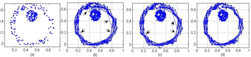
Exp. 1. Graph Construction Performance:
Here we use a similar syntactic data in (Jebara et al., 2009) shown in Fig.2.a, which contains two clusters of dissimilar densities and shapes. We investigate three graph construction methods, lin-eark-neighborhoods of (Roweis and Saul, 2000) in Fig.2.b, b-matching(Jebara et al., 2009) in Fig.2.c and RLN of this work in Fig.2.d using a dataset of 300 points with binary output values. b-matching permits a given datum to selectkneighboring points but also ensures that exactlyk points selects given datum as their neighbor.
Figure 2: Graph Construction Experiments. (a) Syntactic data. (b) lineark-neighborhood (c) b-matching (d) RLN.
In Fig. 2.d, RLN can separate two classes more efficiently than the rest. Compared to the b -matching approach, RLN clearly improves the ro-bustness. There are more links between clusters in other graph methods than RLN, which shows that RLN can separate two classes much efficiently. Also since dynamic number of edges are constructed with RLN, unnecessary links are avoided, but for the rest of the graph methods there are edges between far away nodes (shown with arrows). In the rest of the experiments, we use b-matching for benchmark as it is the closest approach to the proposed RLN.
Exp. 2. Semantic Component Recognition:
We demonstrate the performance of the new RLN with two sets of experiments for sequence labeling of question recognition task. As a first step in un-derstanding semantic components of questions, we asked two annotators to annotate a random subsam-ple of 4000 TREC factoid and description questions obtained from tasks of 1999-2006. There are 11 predefined semantic categories (section 3), close to 280K labeled tokens. Annotators are told that each question must have one topic and zero or one focus and event, zero or more of the rest of the compo-nents. Inter-tagger agreement is κ = 0.68, which denotes a considerable agreement.
We trained models on 3500 random set of ques-tions and reserved the rest of 500 for testing the per-formance. We applied pre-processing and feature selection of section 3 to compile labeled and unla-beled training and launla-beled testing datasets. At train-ing time, we performed manual iterative parameter optimization based on prediction accuracy to find the best parameter sets, i.e., k = {3,5,10,20,50}, ∈ {0,1}, distance ={linear, gaussion}.
We use the average loss (L¯) per sequence (query)
other topic focus event rest
# Samples 1997 1142 525 264 217
[image:7.612.98.522.77.174.2]CRF 0.935 0.903 0.823 0.894 0.198 b-matching 0.871 0.900 0.711 0.847 0.174 RLN 0.911 0.910 0.761 0.834 0.180
Table 2: Chunking accuracy on testing data. ’other’=O,
’topic’=BT+IT, ’focus’ = BF+IF, ’event’= ’BE+IE”,
’rest’= rest of the labels, i.e., IE, BC, IC, BCL, ICL.
to evaluate the semantic chunking performance:
¯
L= N1 PNi=1hL1
i
PLi
j=1I(( ˆyi)j 6= (yi)j) i
(21)
whereyˆandyare predicted and actual sequence re-spectively;N is the number of test examples;Li is the length ofithsequence;Iis the 0-1 loss function.
(1)Chunking Performance:Here, we investigate the accuracy of our models on individual component prediction. We use CRF, b-matching and our RLN to learn models from labeled training data and eval-uate performance on testing dataset. For RLN and b-matching we use training as labeled and testing as unlabeled dataset in transductive way to predict to-ken labels. The testing results are shown in Table 2 for different group of components. The accuracy for ’topic’ and ’focus’ components are relatively high compared to other components. Most of the errors on the ’rest’ labels are due to confusion with ’topic’ or ’focus’. On some components, i.e.,topic,other, RLN performed significantly better than b-matching based on t-test statistics (at 95% confidence). No statistical significance between CRF and RLN is ob-served indicating that RLN’s good performance on individual label scoring, as it shows that RLN can be used efficiently for sequence labeling.
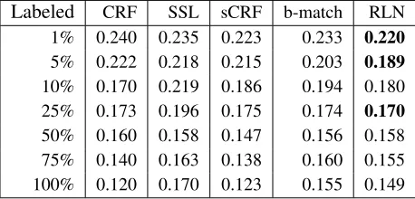
Labeled CRF SSL sCRF b-match RLN
1% 0.240 0.235 0.223 0.233 0.220
5% 0.222 0.218 0.215 0.203 0.189
10% 0.170 0.219 0.186 0.194 0.180
25% 0.173 0.196 0.175 0.174 0.170
50% 0.160 0.158 0.147 0.156 0.158
75% 0.140 0.163 0.138 0.160 0.155
100% 0.120 0.170 0.123 0.155 0.149
Table 3: Test Data Average Loss on graph construction with RLN, b-matching, standard SSL with kNN as well as CRF, CRF with Self Learning (sCRF).
demonstrated that RLN is an alternative method to the standard sequence learning methods for the question labeling task, next we evaluate per sequence (question) performance, rather than in-dividual label performance using unlabeled data. Firstly, we randomly select subset of labeled train-ing dataset,XLi ⊂ XL with different sample sizes,
niL = 5%∗nL, 10%∗nL, 25%∗nL, 50%∗nL,
75%∗nL,100%∗nL, wherenLis the size ofXL. Thus, instead of fixing the number of labeled records and varying the number of unlabeled points, we pro-pose to fix the percentage of unlabeled points in training dataset. We hypothetically use unselected part of the labeled dataset as unlabeled data at each random selection. We compare the result of RLN to other graph based methods including standard SSL (Zhu et al., 2003) using kNN, and b-matching. We also build a CRF model using the same features as RLN except the output information, which CRF learns through probabilistic structure. In addition, we implemente self training for CRF (sCRF), most commonly known SSL method, by adding most con-fident(x, f(x))unlabeled data back to the data and repeat the process 10 times. Table 3 reports average loss of question recognition tasks on testing dataset using these methods.
When the number of labeled data is small (niL < 25%nL), RLN has better performance compared to the rest (an average of 7% improvement). The SSL and sCRF performance is slightly better than CRF at this stage. As expected, as the percentage of labeled points in training is increased, the CRF outperforms the rest of the models. However, observing no sta-tistical significance between CRF, b-matching and
[image:8.612.72.301.73.183.2]# Unlabeled tokens 25K 50K 75K 100K Average Loss 0.150 0.146 0.141 0.139
Table 4: Average Loss Results for RLN graph based SSL as unlabeled tokens is increased.
RLN up to 25-50% labeled points indicates RLNs performance on unlabeled datasets. Thus, for se-quence labeling, the RLN can be a better alternative to known sequence labeling methods, when manual annotation of the entire dataset is not feasible.
Exp. 3. Unlabeled Data Performance: Here we evaluate the effect of the size of unlabeled data on the performance of RLN by gradually increas-ing the size of unlabeled questions. The assump-tion is that as more unlabeled data is used, the model would have additional spatial information about to-ken neighbors that would help to improve its gener-alization performance. We used the questions from the Question and Answer pair dataset distributed by Linguistic Data Consortium for the DARPA GALE project (LDC catalog number: LDC2008E16). We compiled 10K questions, consisting of 100K tokens. Although the error reduction is small (Table 4), the empirical results indicate that unlabeled data can have positive effect on the performance of the RLN method. As we introduce more unlabeled data, the RLN performance is increased, which indicates that there is a lot to discover from unlabeled questions.
8 Conclusions
References
A. Alexandrescu and K. Kirchhoff. 2007. Data-driven graph construction for semi-supervised graph-based learning in nlp. InProc. of HLT 2007.
M. Belkin and P. Niyogi. 2002a. Laplacian eigenmaps and spectral techniques for embedding and clustering. In Advances in Neural Information Processing Sys-tems.
M. Belkin and P. Niyogi. 2002b. Using manifold struc-ture for partially labeled classification. In Proc. of NIPS 2002.
M. Belkin, P. Niyogi, and V. Sindhwani. 2006. A ge-ometric framework for learning from examples. In
Journal of Machine Learning Research.
J. D. Burger. 2006. Mitre’s qanda at trec-15. InProc. of the TREC-2006.
J.Y. Chai and R. Jin. 2004. Discourse structure for context question answering. InProc. of HLT-NAACL 2004.
O. Delalleau, Y. Bengio, and N.L. Roux. 2005. Efficient non-parametric function induction in semi-supervised learning. InProc. of AISTAT-2005.
H. Duan, Cao Y, C.Y. Lin, and Y. Yu. 2008. Searching questions by identifying question topic and question focus. InProc. of ACL-08.
S. Fan, Y. Zhang, W.W.Y. Ng, Xuan Wang, and X. Wang. 2008. Semantic chunk annotation for complex ques-tions using conditional random field. InColing 2008: Proc. of Workshop on Knowledge and Reasoning for Answering Questions.
GD. Forney. 1973. The viterbi algorithm. InProc. of IEEE 61(3), pages 269–278.
A. Goldberg and X. Zhu. 2009. Keepin’ it real: Semi-supervised learning with realistic tuning. In Proc. of NAACL-09 Workshop on Semi-Supervised Learning for NLP.
E. Hajicova, P. Sgall, and H. Skoumalova. 1993. Iden-tifying topic and focus by an automatic procedure. In
Proc. of the EACL-1993.
T. Jebara, J. Wang, and S.F. Chang. 2009. Graph con-struction and b-matching for semi-supervised learning. InProc. of ICML-09.
Dan Klein and Christopher D. Manning. 2003. Accu-rate unlexicalized parsing. InProceedings of the 41st Meeting of the ACL-2003, pages 423–430.
J.D. Lafferty, A. McCallum, and F. Pereira. 2001. Con-ditional random fields: Probabilistic models for seg-menting and labeling sequence data. InProc. of 18th International Conf. on Machine Learning (ICML’01). M. Maier and U.V. Luxburg. 2008. Influence of graph
construction on graph-based clustering measures. In
Proc. of Neural Infor. Proc. Sys. (NIPS 2008).
M.-C.D. Marneffe, B. MacCartney, and C.D. Manning. 2006. Generating typed-dependency parsers from phrase structure parsers. InIn LREC2006.
S.T. Roweis and L.K. Saul. 2000. Nonlinear dimension-ality reduction by locally embedding. InScience, vol-ume 290, pages 2323–2326.
F. Wang and C. Zhang. 2006. Label propagation through linear neighborhoods. InProc. of the ICML-2006. Dengyong Zhou, Olivier Bousquet, Thomas N. Lal,
Ja-son Weston, and Bernhard Scho¨lkopf. 2004. Learning with local and global consistency. Advances in Neural Information Processing Systems, 16:321–328. Xiaojin Zhu, John Lafferty, and Zoubin Ghahramani.