A Novel Methodology for Simulating Contact Line Behavior in Capillary Driven Flows

(1)

A Novel Methodology for Simulating Contact-Line Behavior

in Capillary-Driven Flows

Thesis by

Gerry Della Rocca

In Partial Fulfillment of the Requirements for the Degree of

Doctor of Philosophy

California Institute of Technology Pasadena, California

2014

(2)

(3)

(4)

Acknowledgments

An investment in knowledge pays the best interest.

— Benjamin Franklin

I would first like to thank my doctorate advisers. My official adviser, Professor G. Blanquart, had a critical guiding role in this work despite (or perhaps because of) all our friction and email storms. I really grew as an individual and as a researcher working with him. While most people are limited to a single adviser, I had the privilege of two additional unofficial advisers. I worked with Professor S. M. Troian for approximately a year in the middle of my doctorate and while none of that research appears in the present work, my experience with her was invaluable. It may have arguably been the turning point in my graduate school career. Professor T. Colonius has been a great counselor; I could always count on blunt, honest, and fair criticism even if I didn’t want to hear it.

(5)

My elder brother, Joe, has had a dynamic impact on my life. I cannot claim to have been a good younger brother; I certainly didn’t look up to him growing up and saying a loathed him wouldn’t be far from the truth. I pushed myself to beat him in every way. This competition created the person I am today. Surprisingly, I realized a few years ago that, regardless of our differences, I’m really proud to call him my brother. These are words I never thought I’d write.

Lastly, I could not have gotten where I am without my parents. My parents (Vin and Pam) have always emphasized education’s importance. I learned at an early age that, while they would never buy me video games, they would buy me any book I wanted. Additionally, they sacrificed much to get me through an expensive high school and college. I hope I can be worthy of this exceptional investment and support.

(6)

Abstract

Despite the wide swath of applications where multiphase fluid contact lines exist, there is still no consensus on an accurate and general simulation methodology. Most prior numerical work has im-posed one of the many dynamic contact-angle theories at solid walls. Such approaches are inherently limited by the theory accuracy. In fact, when inertial effects are important, the contact angle may be history dependent and, thus, any single mathematical function is inappropriate. Given these lim-itations, the present work has two primary goals: 1) create a numerical framework that allows the contact angle to evolve naturally with appropriate contact-line physics and 2) develop equations and numerical methods such that contact-line simulations may be performed on coarse computational meshes.

(7)

To capture contact-line physics, two classical boundary conditions, the Navier-slip velocity boundary condition and a fixed contact angle, are implemented in direct numerical simulations (DNS).DNS are found to converge only if the slip length λis well resolved by the computational mesh. Unfortunately, since λ is often very small compared to fluid structures, these simulations are not computationally feasible for large systems. To address the second goal, a new methodology is proposed which relies on the volumetric-filtered Navier-Stokes equations. Two unclosed terms, an average curvature κ¯ and a viscous shear VS, are proposed to represent the missing microscale physics on a coarse mesh.

(8)

List of Figures

1.1 Contact line in 2D between fluid 1 and fluid 2. θis the contact angle. . . 2

1.2 a) Lotus leaf [17]. b) Namibian beetle [106]. Images reproduced with permission from the Nature Publishing Group under licenses3374961113213and3374931001319. . . 2

1.3 Diagram of the interfacial surface tensions for Young’s equation (Eq. 1.1). θS is the equilibrium contact angle. . . 3

1.4 a) Apparent contact angle θapp for a liquid droplet. b) Dynamic contact angleθD at the microscale. . . 5

1.5 Diagrams for the different reinitialization schemes. (•) are the marker particles in a front-tracking method. Note: the values in (b) and (c) are for illustration only. . . 9

2.1 Diagram of a 2 cell thick shell around a circle. The numbers and colors represent different band numbersBa. . . 28

2.2 Cells used in the least square polynomial fit in 3D: a) 19 cells centered on the point of interest (non-wall), b) pyramid shaped collection of cells with the point of interest in the middle of the base (wall). . . 30

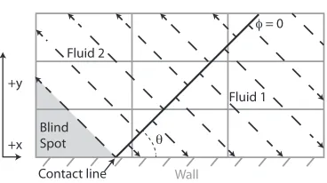
3.1 Diagram of the blind spot (grey). The black solid line corresponds to the interface

φ= 0. The dashed lines are the characteristics for the Hamilton-Jacobi equation which are perpendicular to the interface. . . 32

(14)

3.3 Test case geometries for (a) a wedge and (b) a circular arc. The coordinate system is centered in the domain of width L and height H. . . 34

3.4 Interface profiles with no reinitialization as a function of time, t (pure transport at a constant speed). . . 37

3.5 Integrated error Ep and angle at the wall θ as functions of time for both the wedge (dashed line) and circular arc (solid line) when the level set function is not reinitialized. 37

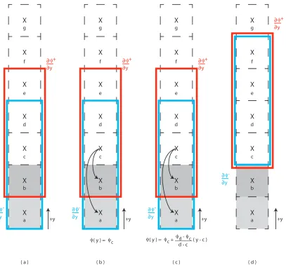
3.6 Diagram of the finite-difference stencil variations used in the presence of a wall: a) standard WENO stencil points for the upwind∂φ/∂y+ _{(red) and downwind} _∂φ/∂y−

(blue) directions, b) zero Neumann boundary condition, c) extrapolation method, d) shifted stencils around point c or d that exclude the wall. The solid line boxes surround the points used in the stencil. The shaded cells a and b are in the wall. . . 39

3.7 Interface profiles when a zero Neumann boundary condition is used. . . 40

3.8 Integrated error Ep and angle at the wall θ as functions of time for both the wedge (dashed line) and circular arc (solid line) when a zero Neumann boundary condition is used.. . . 41

3.9 Interface profiles when the level setφin the wall is populated using a ghost interface. 42

3.10 Integrated error Ep and angle at the wall θ as functions of time for both the wedge

(dashed line) and circular arc (solid line) when the level setφin the wall is populated using a ghost interface. . . 42

3.11 Interface profiles when the relaxation equation is used for cells on the wall in the blind spot.. . . 46

3.12 Integrated errorEpand angle at the wallθas functions of time for the circular arc when

(15)

3.13 Isocontours for concentric circles during reinitialization for an incorrectly scaled dis-tance function by a factor of a) 1/2 and b) 2. Neighboring isocontours differ by ∆φ= 0.1. The black circular dots indicate the zero level set. . . 48

3.14 Diagram of the 2D and 3D computational domain and initial condition for the droplet on a wall simulations (not drawn to scale). The initial contact angle is 90o. Gravity is oriented parallel to the wall. . . 52

3.15 Deformation of a two dimensional semicircle and full droplet under gravity. The red line is the interface for a droplet on a wall (black line) and the blue dashed line is a full droplet in free fall.. . . 53

3.16 Deformation of the hemispherical droplet sliding under gravity. . . 54

3.17 a)x-y profile and b) Droplet contact line for a 3D droplet. The profiles are overlaid to intersect at the leading edge. . . 54

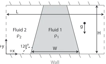
3.18 Diagram of the computational domain and initial conditions for the simulation with merging contact lines (not drawn to scale). Gravity is oriented perpendicular to the walls. . . 56

3.19 Time images of the spreading trapezoidal fluid block (blue) trapped between two walls (brown).. . . 56

4.1 Domain diagram around a contact line. The shaded region is the blind spot where no characteristics (dashed lines) exist to trace the value of un. A, B, C, D, and P are points referenced in the text. Numbers correspond to the band valueBa at the cell centers. The red arrow indicates the direction of the propagated angle ˜θ(Sec. 4.2.2.2). 60

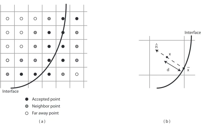
4.2 a) Example diagram for the FMM. Accepted, neighboring, and far points are black, grey, and white respectively. b) Diagram for computing the nearest interface point ˜x. 63

(16)

4.4 a) Domain spurious velocity errorED and b) wall spurious velocity errorEW as

func-tions of time when a fixed angle ˜θis propagated (method 1). Data sets differ by grid resolution. The multiplication factor is relative to the base resolution (125H cells in thex-direction). . . 68

4.5 a) Domain spurious velocity errorED and b) wall spurious velocity errorEW as func-tions of time when the angle ˜θpropagated linearly (method 2). Data sets differ by grid resolution. The multiplication factor is relative to the base resolution (125H cells in thex-direction). . . 68

4.6 Domain spurious velocity error ED as a function of the grid resolution ∆x/H for

method 2 at time t = 2. The red dashed line is the behavior when ED is linearly proportional to the grid cell size. . . 68

4.7 Configuration for a pinned droplet deformed by gravity in the positivex-direction (not drawn to scale). . . 69

4.8 a) Diagram of an interfaceh(x) pinned to the wall (not drawn to scale). b) Variation of the solution interface shape with Bond numberBoW for fixed ¯x0. . . 71

4.9 a) Variation of the solution interface shape with ¯x0 for fixed Bond number BoW. b)

Interface slope∂h/∂xfor the interfaces in (a). . . 71

4.10 a) Initial (red squares) and steady state (blue circles) surface shapes. b) Comparison on the solution for Eq. 4.13 (curve) and the numerical simulation (dots) for aBoW = 3.16

and ¯x0=−0.0296. . . 73

4.11 a) Integrated errorEP for a circular arc (Sec. 3.3). b) Equilibrium surface using the QUICK transport scheme and the reinitialization routines with angle ˜θ(Sec. 4.4). . . 75

(17)

5.2 a) Diagram of the staggered grid. C is the locations of cell centered variables andu,

v are the face centered velocity locations. The blue and red rectangles are the control volumes (box filters)V centered onuand v, respectively. b) 2D box filter of size ∆x

x ∆y containing the contact line. L, R, T, andB denote the four cell sides. PointP

is the grid node about which the control volume is centered. . . 81

5.3 2D Cartesian capillary tube domain for the DNS of contact line dynamics (not drawn to scale). . . 84

5.4 Diagram of the geometry when calculating the average interface curvature. The in-terface intersects the wall at the static contact angleθS and has an angle θ at point P. . . 87

5.5 Results for = 1/40, θS = 50o_{, and} _Ca _{= 0}_._{01. a) Interfaces profiles at} _t _{= 0 and}

at steady state. b) The actual curvature κ at a given y location (black circles), the average curvature ¯κfrom the DNS (red squares), and the average curvature ¯κfrom Eq. 5.10 (blue diamonds). Thex-axis of the plot is distance from the wall in slip lengths. 90

5.6 Results for = 1/40, θS = 90o, and Ca = 0.01. a) Interfaces profiles at t = 0 and

5.7 Results for = 1/40, θS = 50o_{, and} _Ca _{= 0}_._{03. a) Interfaces profiles at} _t _{= 0 and}

5.8 Results for = 1/80, θS = 50o, and Ca = 0.01. a) Interfaces profiles at t = 0 and

(18)

5.9 Example microscopic velocity ¯uS along the solid wall. f and g are functions for the

left and right hand sides of the peak, respectively. . . 94

5.10 Diagrams of the integrated quantitiesF (squares) andG(circles) as functions of contact angle θ, slip length ratio , and capillary number Ca. Colors denote different values of the slip length ratio . The different figures are different Ca : a) Ca = 0.0033, b)

Ca= 0.01, c)Ca = 0.03. . . 97

5.11 Ratiosγ of the data in Fig. 5.10 for all data sets. The set definitions are: Set 1 (red squares) = ratio of F in Figs. 5.10b and 5.10a, Set 2 (blue diamonds) = ratio of F in Figs. 5.10c and 5.10b, Set 3 (black circles) = ratio of G in Figs. 5.10b and 5.10a, Set 4 (green triangles) = ratio of G in Figs. 5.10c and 5.10b. . . 98

5.12 Value ofF andGas a function of slip length ratioforθS = 50o_and_Ca _{= 0}_._{01. The}

lines are a power-law fitAB _{to the data.} _{. . . .} ₉₈

5.13 a) Approximate value ofB(θ) from the data in Fig. 5.10b. b) Approximate value of

A(θ) afterB(θ) is removed fromF (squares) andG(circles). . . 99

6.1 a) Numerical drop contact diameterDC in timetfor model I compared to the

experi-mental data from Fig. 9 in Yokoi et al. [166]. b) Labeled features for the drop impact process. . . 104

6.2 Cylindrical geometry for a droplet impacting on a flat wall (not drawn to scale). The two fluids are water (droplet) and air (surrounding fluid) with the given properties. The droplet has an initial velocityUiin the negativez-direction and an initial distance

XS from the wall. Gravity is oriented in the negativez-direction. The walls at the top and bottom of the domain have no slip velocity boundary conditions. . . 107

6.3 Drop contact diameterDC in timetfor a set static contact angle of 90oin the average

(19)

6.4 Cross-section and revolved surfaces for the water droplet with a set static contact angle of 90o_{in the average curvature ¯}_κ_{and no additional viscous shear VS. The 2D and 3D}

images are not the same scale. The 3D images are taken at a slight angle relative to the side profile and do not include the satellite droplet. . . 109

6.5 Drop contact diameterDC in timetfor a set static contact angle of 90oin the average curvature ¯κat different values of the shear factor β. Approximate values of the slip length ratio are given with each valueβ. The black dots are the experimental data of Fig. 9 in YVHH. . . 110

6.6 Shear factorF (Eq. 5.27) as a function of the slip length ratiofor the static advancing and receding angles. Note: thex-axis is logarithmic. . . 111

6.7 Drop contact diameterDCin timetfor a set contact angle hysteresis anglesθsa= 107o_, θsr = 77o_{in the average curvature ¯}_κ_{and a set shear factor}_β_{. The black dots are the}

experimental data of Fig. 9 in YVHH. . . 112

6.8 Drop contact diameterDC in timetfor a set static contact angle of 90oin the average curvature ¯κand the contact angle hysteresis angles θsa= 107o,θsr = 77oin the shear

factorF. The black dots are the experimental data of Fig. 9 in YVHH. . . 112

6.9 Drop contact diameter DC in time t using the contact angle hysteresis angles θsa =

107o_,_θsr_{= 77}o_{in the average curvature ¯}_κ_{and the shear factor}_F_{. The black dots and}

black dashed line are the experimental data and model I data from Fig. 9 in YVHH, respectively.. . . 113

6.10 Drop images from Fig. 8 in YVHH compared to simulation images from Fig. 6.9 at t = 0, 2, 4, 10, 15, and 30 ms. The camera for images is at a slight angle to mimic the reflection observed in the experimental images. The experimental images are reproduced with permission under license3375611208717. . . 113

6.11 Drop contact diameterDCin timetusing the contact angle hysteresis anglesθA= 107o_, θR= 77o_{. The curves are different grid resolutions. The black dots are the experimental}

(20)

107o_, _θ

sr = 77o. The curves are drops started at different positions XS. The black

dots are the experimental data of Fig. 9 in YVHH. . . 116

6.13 Drop contact diameter DC in time t using the contact angle hysteresis angles θsa = 107o, θsr = 77o. The curves are drops with different initial velocities Ui. The black dots are the experimental data of Fig. 9 in YVHH. . . 117

107o_, _θ

sr = 77o in the average curvature. The shear factors βa and βr are varied

independently for the advancing and receding contact lines. The black dots are the experimental data of Fig. 9 in YVHH. . . 117

C.1 Evolution of the apparent contact angle θapp in time for Ca = 0.01, = 1/40, and

(21)

List of Tables

4.1 Leading and trailing contact angles for the pinned droplet. The angles were estimated using a quadratic polynomial.. . . 73

5.1 Values for the capillary numberCa and static contact angleθS in Fig. 5.5 – 5.8. . . . 89

6.1 Simulation inputs for the average mean curvature and viscous shear VS. . . 106

6.2 Assumptions in Chap. 5 . . . 114

(22)

Nomenclature

AMG Algebraic multigrid.

AMR Adaptive mesh refinement.

BiCGStab Bi-conjugate gradient-stabilized.

CFL Courant-Friedrichs-Lewy number. This value specifies whether a numerical discretization is stable for a given grid spacing ∆xand time step ∆t.

CSF Continuum surface force.

DNS Direct numerical simulation. In this type of simulation, node grid-spacing is smaller than all relevant length scales.

FMM Fast Marching Method.

GFM Ghost fluid method.

HCR2 Modified reinitialization routine proposed by Hartmann et al. [59]. LHS Left hand side of the equation.

LSQ A least-square polynomial fit to the local level set field to approximate derivatives, interface normals, and curvature.

MAC Marker-and-cell.

MD Molecular dynamics.

(23)

QUICK Quadratic upstream interpolation for convective kinematics [86]. This numerical scheme is an Eulerian approach to the advection equation.

SMG Streaming multigrid.

VOF Volume of fluid.

VS Viscous shear term (Eq. 5.7).

WENO Weighted essentially non-oscillatory.

YVHH Short-hand notation for Yokoi et al. [166].

A(θ) Leading coefficient in the power-law approximation for shear factors F and G.

B(θ) Exponent in the power-law approximation for shear factors F and G.

Ba Signed band number.

Bo Bond number = ∆ρgH2/σ for an appropriate length scaleH.

BoW Bond number using length scaleW.

C Color function in the VOF and phase-field methods.

Ca Capillary number =µU/σfor an appropriate velocity U.

D Droplet diameter.

DC Droplet contact (splat) diameter during the droplet impact and spreading process.

Dextrap Extrapolated value of the distance function into a wall.

Dghost Approximate distance function calculated from a ghost interface.

Dω Tangential derivative along a wall.

ED Maximum spurious velocity magnitude throughout the entire domain.

(24)

EW Maximum spurious velocity magnitude along the solid wall.

F In Chap. 2, the forcing function for the HCR2 scheme (Eq. 2.22). In Chap. 5 and 6, the integral of f expressed by Eq. 5.21.

FY oung Unbalanced Young’s force (Eq. 1.2).

G Integral of g expressed by Eq. 5.22.

H Height of a computational domain in they-direction.

I Identity matrix.

L Computational domain length in thex-direction.

LM Large length scale.

La Laplace number =σρH/µ2 for an appropriate length scaleH.

M(C) Mobility parameter in the phase-field method.

N A positive integer.

Oh Ohnesorge number =µ/√ρσH for an appropriate length scaleH.

R Geometric radius of a circular interface.

Re Reynolds number =ρU H/µfor an appropriate length scaleH and velocityU.

S Box filter surface.

T Absolute fluid temperature.

U Constant advection speed used in the wedge and circular arc test cases.

UCL Contact line velocity. In Sec. 5.3, it is also the mean inlet velocity.

Ui Initial droplet velocity.

(25)

We Weber number=ρU2_H/σ_{for an appropriate length scale}_H _{and velocity}_U_.

XS Starting location of initial condition in Chap. 5. Initial droplet height in Chap. 6. Zitterbewegung Trembling motion, from German.

A Normalized, sheared droplet cross-sectional area. The area is normalized byW2_.

D Deviatoric stress tensor.

H Heaviside function.

V Volume of grid cell.

∇s Surface gradient operator along the wall.

∇2

s Surface Laplacian operator along the wall.

∆t Simulation time step.

∆x Grid cell size in the x-direction.

∆φ Change in the level setφ.

Φ Obtuse side indicator (Eq. 3.2).

a1 Constant number.

a2 Constant number.

c Positive constant.

d Approximate distance to the interface.

f(¯x,Ca, , θS) Function representing the microscopic velocity curve ¯uS for the fluid with contact

angleθS.

g(¯x,Ca, ,180o₋_θ

S) Function representing the microscopic velocity curve ¯uS for the fluid with

(26)

g Magnitude of the gravity vector. In Eq. 1.5,g is the known function from Cox [28]. ~g Gravitational acceleration vector.

h(x) Dimensional height profile of the drop as a function of the spatialx-coordinate.

¯

h Dimensionless height profile of the drop as a function of the spatialx-coordinate.

k Number of level set bands.

ka Material-related advancing parameter in model I (Eq. 6.1) from Yokoi et al. [166].

kb Boltzmann constant, 1.38·10−23m2kg s−2K−1.

kr Material-related receding parameter in model I (Eq. 6.1) from Yokoi et al. [166].

m(a, b) Function which returns the input argument with the smaller absolute value.

n Coordinate in the outward normal direction to a wall.

ˆ

n Direction vector normal to the level set isocontours.

~

n Direction vector normal to a solid surface.

p Local fluid pressure.

r Radial cylindrical coordinate.

sgn -1/+1 depending on the orientation of the wall.

t Simulation time variable.

tend End simulation time.

ˆ

t1 First vector tangential to the fluid interface.

ˆ

t2 Second vector tangential to the fluid interface.

u x-component of the velocity vector~u.

(27)

un Extension velocity and normal component of the velocity vector~uto the level set interface.

uS Microscopic velocity component.

utan Wall tangential velocity component of the extension velocityun.

¯

uS Non-dimensional fluid velocity, ¯uS=uS/(UCL−UB).

ˆ

u General velocity vector.

~

u Local fluid velocity vector.

v y-component of the velocity vector~u.

w z-component of the velocity vector~u.

x Cartesian coordinate.This coordinate is often tangential to the solid walls in the present work.

xint x-coordinate for the interface in Chap. 3and4.

x0 Constant in the surface evolution equation that is related to the droplet volume.

¯

x Non-dimensional x-coordinate centered ata, ¯x= (x−a)/λ.

¯

x0 Dimensionless constant in the surface evolution equation that is related to the drop volume.

ˆ

x Non-dimensional x-coordinate, ˆx=x/λ.

˜

x Closest point on the interface to a grid node.

~

x Spatial location vector for a target point.

~

x1 Spatial location vector for an accepted neighbor point in the FMM.

y Cartesian coordinate. This coordinate is often normal to the solid walls in the present work.

z Axial cylindrical coordinate or the third Cartesian coordinate.

α Angle of the circular arc initial condition.

(28)

βa Shear factor β for advancing contact lines.

βr Shear factorβ for receding contact lines.

γ Ratio of shear rate factors at different capillary numberCa.

δ Dirac delta function. In Eq. (2.22), it is a small parameter.

Ratio of a small and large length scale. The small length scale is usually the slip lengthλand the large length scale either H or R.

C Width of the fluid-fluid interface for the phase-field method.

η Fluid density ratioρ2/ρ1.

θ Isocontour angle. For the zero isocontour, it is the contact angle.

θapp Macroscale apparent contact angle.

θD Microscale dynamic contact angle.

θm Microscale contact angle.

θmax Maximum contact angle θ allowed as a target angle in the relaxation equation (Eq. 3.5).

Throughout this study, it is 170o_.

θmda Maximum advancing contact angle in model I (Eq. 6.1) from Yokoi et al. [166].

θmdr Minimum receding contact angle in model I (Eq. 6.1)from Yokoi et al. [166].

θmin Minimum contact angle θ allowed as a target angle in the relaxation equation (Eq. 3.5).

Throughout this study, it is 10o_.

θo Contact angle prior to reinitialization.

θS Static (equilibrium) contact angle.

θsa Static advancing contact angle.

(29)

˜

θ Propagated value of the isocontour angleθin the blind spot.

˜

θmax Maximum value of the propagated angle ˜θallowed.

˜

θmin Minimum value of the propagated angle ˜θallowed.

κ Interface curvature.

κapp Curvature applied in the GFM at the contact line.

κ0 Frequency of molecular displacements.

κ1 First mean curvature component, the standard 2D Cartesian coordinate curvature.

κ2 Second mean curvature component, the curvature associated with the cylindrical surface.

¯

κ Average curvature.

λ Slip length in the Navier-slip boundary condition.

µ Dynamic fluid viscosity.

µC Rate of change of free energy in the phase-field method.

µef f Effective dynamic viscosity at a contact line.

ξ Fluid viscosity ratioµ2/µ1.

ρ Fluid density.

σ Coefficient of surface tension.

σs1 Free energy between the solid surface and fluid 1 in Young’s equation (Eq. 1.1).

σs2 Free energy between the solid surface and fluid 2 in Young’s equation (Eq. 1.1).

τ Pseudo-time variable for iterating the reinitialization equation.

τCa Capillary time scale,µH/σ.

τW e Inertial-capillary time scale, p

(30)

υ Average displacement distance in molecular kinetic theory.

φ Level set variable. In this work, it is a signed distance function.

φtemp Temporary value of the level setφ.

φ0 Value of the level setφprior to reinitialization.

ψ In Chap. 1, the bulk energy density in the Cahn-Hilliard equation (Eq. 1.7). In Chap. 2, the height fraction of fluid 1.

(31)

Chapter 1

Introduction

... not even Herakles could sink a solid if the physical model were

entirely valid ...

— Huh and Scriven [67]

1.1 Motivation

Contact lines, the intersection of three immiscible material phases, are ubiquitous throughout na-ture and industrial applications. A contact line in 2D is a point and in 3D is a contour. Usually, in fluid mechanics, the contact-line phenomenon refers to the location where two fluids meet on a solid wall at a contact angle θ (Fig. 1.1). In capillary-driven fluid flows (large surface tension σ, small characteristic length scale), the contact-line behavior can control the flow. This thesis aims to develop a numerical framework where flows affected by contact lines can be studied and optimized efficiently. Interest in contact lines can be broken into three classes, namely understanding nature, industrial applications, and fundamental science.

Understanding nature:

(32)

Solid Wall θ

Fluid 1 Fluid 2

Contact line

Figure 1.1: Contact line in 2D between fluid 1 and fluid 2. θ is the contact angle.

[image:32.612.247.401.64.173.2]

( a ) ( b )

Figure 1.2: a) Lotus leaf [17]. b) Namibian beetle [106]. Images reproduced with permission from the Nature Publishing Group under licenses3374961113213and3374931001319.

tools. Indeed, artificial surfaces have already been inspired by these leaves [17]. While lotus leaves repel water, other organisms such as beetles in the Namib Desert (Fig. 1.2b) have surfaces that collect water [55]. The beetle’s wings have alternating hydrophobic and hydrophilic patches where water is gathered from the surrounding desert air [106]. This structure would be useful in fresh water condensers.

Industrial applications:

(33)

Solid Wall

θ_S

Fluid 1 Fluid 2

σ σs2

[image:33.612.245.401.67.174.2]

σs1

Figure 1.3: Diagram of the interfacial surface tensions for Young’s equation (Eq. 1.1). θS is the

equilibrium contact angle.

in polymer-electrolyte-membrane fuel cells [76,150], and reaction control in microreactors [75]. With energy demands expected to rise by a third in the next 25 years [5], it is critical to maximize energy resource usage. While porous media are the ideal target, the first two cases should be developed beforehand due to their relative simplicity. These simpler cases will be used in the present work.

Fundamental science:

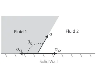
Despite their omnipresence and importance, understanding of contact lines is limited. Young [167] proposed the traditional formulation for the static contact angle θS at equilibrium which is now referred to as Young’s equation (Fig. 1.3):

σs2+σcos(θS) =σs1 (1.1)

The free energies per unit area σ, σs1, and σs2 are material properties and in thermodynamic

equilibrium. Young’s equation is only valid at equilibrium. Away from equilibrium, a new dynamic contact angle θD forms. This angleθD is sometimes represented by the unbalanced Young’s force FY oung,

FY oung=σ(cos(θS)−cos(θD)) (1.2)

(34)

concept of no slip were indeed strictly valid, fluid 1 would never be able to replace fluid 2 along the solid and vice versa (Fig. 1.1). Examining Stokes flow in a liquid wedge at the contact line, Huh and Scriven [67] showed that the no slip boundary condition causes the shear stress to diverge as 1/r, where r is the radial distance along the wall to the contact line. This non-integrable shear stress yields an infinite shear force which inspired the quote at the beginning of this chapter. The interface must be able to move with a contact line velocity UCL. Contact lines challenge the postulates of fluid mechanics (namely the no slip condition) and must be handled differently both analytically and numerically. The following section describes the existing models for this region.

1.2 Prior contact-angle models

(35)

Wall

( a ) θapp

Wall

( b ) θD

θ_app θD

Figure 1.4: a) Apparent contact angleθappfor a liquid droplet. b) Dynamic contact angleθDat the

microscale.

1.2.1 Molecular kinetic theory

Yarnold and Mason [164] first proposed that the relationship between contact line velocityUCLand the dynamic contact angle might be controlled by the molecular statistical dynamics. The driving force is the unbalanced Young’s force (Eq. 1.2) and the contact-line motion occurs due to thermally-driven molecular response. The key parameters are the equilibrium frequency of random molecular displacementsκ0and the average distance of displacementυ. Blake and Haynes [16] quantified the

molecular kinetic theory as

UCL= 2κ0υsinh

_σ(cosθ

S−cosθD)υ2

2kBT

(1.3)

where kb is the Boltzmann constant and T the absolute fluid temperature. Neither of the key parameters in this model can be easily measured and are typically fitted to experimental data.

1.2.2 Hydrodynamic theory

(36)

A common choice to relieve the stress singularity is to use a Navier-slip boundary condition [98],

∂u ∂n =

u

λ (1.4)

whereuis the velocity tangential to a solid wall,nis the direction normal to that wall, andλis the slip length. The slip velocity is proportional to the shear rate which decays away from the contact line. This slip lengthλis estimated to be on the order of nanometers [39,92]; it is related to, but not equal toυ in the molecular kinetic theory.

Matched asymptotic, analytic solutions have been derived in the hydrodynamic framework as the ratio of the micro and macro length scales = Lm/LM → 0 and the capillary number Ca

=µUCL/σ→0 whereµis the fluid dynamic viscosity. Cox [28] derived the apparent contact angle

for a liquid-liquid system as

g(θapp)−g(θm) = Ca·log(

1

) (1.5)

wheregis a known function. The microscale contact angleθmwas set as the static contact angleθS in his analysis. He assumed a no slip boundary condition far away and stated that the slip condition at the contact line (whichever chosen) would only show up as an additional constant. Unfortunately, this relation cannot be used for finite Reynolds number flows (Re =ρUCLLM/µ 6= 0 ), nor when

(37)

1.2.3 Non-unique contact angles

In both the molecular kinetic theory and hydrodynamic models, the contact angle is assumed to be a unique function of material properties and standard parameters: however, there is experimental evidence that implies the contact angle may be multivalued for finite Reynolds number. Blake et al. [15] performed a series of curtain-coating experiments and found that the flow rate of the curtain fluid affected the contact angle. This result implies that the hydrodynamics far away from the contact line are important. For example, in curtain coating, the finite film thickness and its free fluid surface can affect the contact angle. A subsequent study by Clark and Stattersfield [27] found similar results where a recirculation region could form. In addition, a series of experiments and simulations by Ding and Spelt [36], Ding et al. [35], and Sui and Spelt [142] for rapidly spreading drops showed that the apparent contact angle is non-unique when inertial effects are important. Since a single equation cannot easily capture this multivalued function, a simulation framework is sought where the contact angle evolves naturally from all physical effects involved.

1.3 Numerical methods for multiphase flow and contact lines

(38)

1.3.1 Atomistic methods

Atomistic approaches seek to model the interaction of molecular particles and subsequently cap-ture the macroscale fluid behavior [72]. Molecular dynamics (MD) is the most well-known of these techniques. In MD, discrete atoms affect each other through interaction potentials such as the Lennard-Jones potential [85]. All results are subject to the validity of the chosen potential. The macroscale fluid properties such as the flow velocity are calculated from suitable particle averages. Examples of molecular dynamics studies for contact lines are Koplik et al. [79], Thompson and Robbins [151], Qian et al. [112], and Ren and E [115]. The advantages of MDare that it is a very fundamental approach and may capture physics more accurately (particularly on the nanoscale) than continuum methods. Furthermore, it does not require the solution of multidimensional, par-tial differenpar-tial equations. The major disadvantage isMD’s computational expense: computational effort increases linearly with the number of particles and simulation run-time. Historically,MD sim-ulations have been limited to only small collections of molecules [72]. One of the largest simulations to date [51] has 7 orders of magnitude fewer particles than are necessary to simulate a cubic mil-limeter of water. While some hybrid atomistic-continuum simulation methods have been proposed [50,53, 54], other authors argue that these two approaches are inherently incompatible and should not be coupled in this way [132]. WhileMD simulations are useful for probing scientific questions, their applicability to realistic problems is limited.

1.3.2 Continuum methods

(39)

( a ) Front-tracking ( b ) Volume of fluid ( c ) Level set 0 0.15 0.15 0

0.15 0.95 0.95 0.15

0 0.15 0

0.15 0.95 0.95 0.15

0.15

0.7 0.7

-0.2 -0.2

-0.8 -0.8

-0.2 -0.2

-0.8 -0.8

0.7 0.7

-0.2 -0.2

Figure 1.5: Diagrams for the different reinitialization schemes. (•) are the marker particles in a front-tracking method. Note: the values in (b) and (c) are for illustration only.

1.3.2.1 Front-tracking methods

These methods explicitly track the location of the fluid interface, usually using marker particles. A circular interface with marker particles (dots) is shown in Fig. 1.5a. These marker particles are transported with the local fluid velocity in a Lagrangian fashion and the new interface is identified by these points. One of the earliest front-tracking methods is the marker-and-cell (MAC) approach of Harlow and Welch [57] for free surface flows. In theMACmethod, each liquid grid cell was seeded with marker particles. Any cell containing a marker particle after transport was identified as fluid. There is no connectivity between the particles in this formula and they are spread throughout the fluid volume. Unverdi and Tryggvason [154] proposed a front-tracking method using particles only on the interface with known connectivity. The advantages of this method are that it is easy to visualize and the exact location of the interface is known. However, while it is conceptually simple, its implementation is not. Special numerical rules are needed to remove / add marker particles as neighboring particles get too close / far apart. Front-tracking methods have particular difficulties handling merging surfaces; thin fluid filaments will persist unless a devoted routine removes them.

1.3.2.2 Front-capturing methods

(40)

the major benefits of these methods over front-tracking methods is that they naturally handle merg-ing interfaces and topological changes. This benefit comes at the loss of fine scale features on coarse meshes, features that front-tracking methods preserve. Capturing merging interfaces and fine fluid threads are nearly mutually exclusive conditions. Furthermore, whereas front-tracking methods may require special data constructs to store the interface information and connectivity, the scalar values of front-capturing methods are stored like any other scalar variable. These methods, therefore, are easily extended to 3D. Three types of front-capturing methods are volume of fluid, phase field, and level set methods.

Volume of fluid method:

The volume of fluid method (VOF) was first introduced by Hirt and Nichols [62]. VOF methods have been previously used by Renardy et al. [116], Afkhami et al. [3,4], and Dupont and Legendre [37] to simulate contact line movement. In aVOFmethod, each grid cell is assigned a color function C(or volume fraction) that represents the amount of fluid 1 present in the cell. If the cell is entirely fluid 1,C= 1; if it is entirely fluid 2,C= 0. An example of volume fractions for a circular interface is shown in Fig. 1.5b. The color functionC is transported using the advection equation,

∂C

∂t +~u· ∇C= 0 (1.6)

where~uis the local fluid velocity. The primary benefit ofVOFmethods for incompressible flows is that mass is exactly conserved if Eq. 1.6 is reformulated in its conservative form. The major dis-advantage is the difficulty in reconstructing the fluid interface; the interface location is not obvious [121]. This disadvantage raises concerns when calculating interface normals and curvature. If the interface is sharp (an abrupt transition betweenC= 0 and 1), these quantities are poorly calculated.

(41)

with shrinking grid dimensions. Since curvature must be accurate in surface-tension-dominated fluid flows, theVOFmethod is not appropriate for the present work.

Phase field method:

Like VOFmethods, phase-field methods use a color function C to distinguish between fluids. A chemical transport equation, the Cahn-Hilliard equation

∂C

∂t + (~u· ∇)C=∇ ·(M∇µC) , (1.7)

is used instead of Eq. 1.6forVOFmethods [162]. The interface is spread over several cells to indicate the transition layer between the two fluids. M(C)is a diffusion parameter called the mobility. This chemical diffusion is one of the strengths of this approach; the contact line can diffuse along the surface and the contact-line stress singularity is relieved even for a no slip boundary condition. The rate of change of free energy isµC. This parameter contains the two drawbacks of the phase field method. µC is expressed as

µC=

∂ψ ∂C −

2 C∇

2_C _(1.8)

whereC is a width indicative of the fluid-fluid interface thickness andψis the bulk energy density. For realistic cases,C may be very small, requiring high resolution simulations. Furthermore, when Eq. 1.8is used in Eq. 1.7, the Cahn-Hilliard equation contains fourth-order derivatives of the color functionC. These high-order derivatives require special treatment. Examples of studies using the phase field method for multiphase flows are Jacqmin [69,70], Lowengrub and Truskinovsky [88], Yue et al. [169], and Carlson et al. [22].

Level set method:

(42)

computation of isocontour normal vectorsnˆ and curvaturesκ,

ˆ

n= _|∇∇φ_φ_|, κ=−∇ ·nˆ . (1.9)

The level set method is used in the present work for this reason; accurate curvature is important in capillary-dominated fluid flows. Two common choices ofφare a signed distance function (interface φ = 0) [97, 26] and a conservative hyperbolic tangent distance function [100, 170, 34] (interface φ = 0.5). Only the signed distance function, the more common choice in literature, is considered in this work. A signed distance function for a circular interface is shown in Fig. 1.5c. Ifφ > 0, the cell center is in fluid 1; ifφ <0, it is in fluid 2. The mathematical condition for a signed distance function is a unity gradient magnitude,|∇φ|= 1.

The level set functionφis typically evolved in two steps: an advection step and a reinitialization step. First, to transport the interface, the level-set variableφis advected with the local fluid velocity ~

uto determine the new interface location using an advection equation

∂φ

∂t +~u· ∇φ= 0. (1.10)

Unfortunately, after transport, φis in general no longer a distance function. While the simulation can proceed using a non-distance function φ, the constraints (namely, a smooth and continuousφ field) may no longer be satisfied after multiple iterations. If the gradients of φ become large or small, the benefit of accurate curvature is lost. This distortion of level set isocontours caused by fluid motion necessitates the second step, reinitialization [24,145,171].

(43)

front-tracking method (Fig. 1.5a). A grid node’s distance d to each marker is calculated and the smallest value dis set as the new level set magnitude. This direct method is very computationally expensive. In addition, its extension to 3D is non-trivial and requires constructing fluid interface panels [144].

The second approach is Fast Marching Method (FMM) [1, 124, 125]. The FMM solves the Eikonal equation,

|∇φ|2= 1 (1.11)

for the distance function and marches values out from the interface. This method is quite efficient computationally. However, this method is usually only first order accurate. Therefore, the curvature would be less accurate since it requires second-order derivatives ofφ(Eq. 1.9). While second-order FMM methods do exist [124], they are more challenging to implement. Other authors have been unable to extend the FMM to even higher order accuracy; there are finite-difference stencil and stability issues [99].

The third reinitialization technique iterates a partial differential equation in pseudo-timeτ until steady state. A standard equation is the Hamilton-Jacobi equation given by [145]

∂φ

∂τ +sign(φ0) (|∇φ| −1) = 0. (1.12)

φ0 is the value of φprior to reinitialization. This equation is hyperbolic and its characteristics are

normal to the interface φ = 0 (Fig. 3.1). At steady state, |∇φ| = 1, the condition for a signed distance function. This approach is used here because it is more efficient than the direct approach and can use high-order discretizations easily, unlike the FMM.

(44)

is to readjust the value of the level setφafter reinitialization such that the fluid volume before and after reinitialization are equal [137]. This approach may artificially move the fluid interface. Another strategy modifies Eq. 1.12. Russo and Smereka [117] proposed a different discretization with better mass conservation. Hartmann et al. [58,59] added additional source terms to pin the location of the zero level set. In addition, there are several hybrid techniques that couple two techniques: level set and front-tracking [99,133], level set andVOF[94,146], and level set and particle methods [40,61].

1.4 Thesis outline

The first goal of this work isto create a numerical framework that allows the contact angle to evolve naturally with appropriate contact-line physics. Unlike prior work, no dynamic or apparent contact-angle law is strictly applied. Such an approach is particularly useful for cases where the Reynolds number Re and capillary numbers Ca are large since there are no complete theories in these regimes at this time. Furthermore, the multivalued contact angle mentioned in Sec.

1.2.3is not problematic since a contact-angle law is not prescribed. The framework will be derived with certain physical assumptions, but other physical mechanisms can be incorporated if necessary.

The second goal of this work is to develop equations and numerical methods such that contact-line simulations may be run on coarse computational meshes. Surface tension is usually treated explicitly due to the non-linearity of curvature with the level set variable φ (Eq.

(45)

The first goal is accomplished in Chap. 3–5. This goal focuses on reducing numerical errors of existing methods for floating (non-prescribed) contact angles and creating physical source terms. The second goal of computationally efficient simulations is attained in Chap. 5 and6. Contact-line physics are not included in Chap. 3and4; the numerical methods alone are examined. The contact-line physics are reintroduced in Chap. 5.

Chapter2 describes the governing equations for multiphase flow and credits the existing numerical methods that are employed throughout. This chapter may be skipped without loss of continuity.

Before the level set method is used at a contact line, the numerical methods for a freely floating contact angle must be checked to ensure that they do not introduce spurious effects. Chapter 3

resolves a subtle point about level set reinitialization. This has to do with the “blind spot” created near the contact line; this region has no characteristics from the Hamilton-Jacobi equation (Eq.

1.12). A relaxation equation is then proposed that minimizes the errors caused by this ill-posed problem.

Chapter4 expands the concepts of Chap. 3 to level-set extension velocities and offers a solution to ensure correct contact angles in the relaxation equation. The reinitialization technique is completed by supplementing it with an angle propagation algorithm. This combined algorithm is referred to as the relaxation equation reinitialization.

(46)

In Chap. 6, all of the previously derived source terms and numerical methods are combined into a complete framework. Drop impacts are difficult to capture using existing contact angle relations because of the large fluid velocities (Re>1,Ca>1). A drop impact experiment and its simulated counterpart are compared. The slip length λ is adjusted to the experimental data and the value obtained is surprisingly realistic. Good agreement is shown: the methods created here are quite promising.

Chapter7presents a brief summary of this work and suggestions for future extension are discussed.

1.5 Contributions

This work makes the following contributions:

• A new relaxation equation is added to the level-set reinitialization which holds curvature

constant in the blind spot. This technique introduces minimal numerical errors and is easily extended to 3D. (Chap. 3)

• The concept of fixed curvature is included in a new technique to create consistent level-set

extension velocities along the solid boundary. (Chap. 4)

• The level-set relaxation equation is completed by including angle propagation. This surface propagation has not been previously seen in the literature. (Chap. 4)

• The former contributions create a framework where the contact angle can be left floating; it

is determined by the physics. This approach is important for finite Reynolds number effects. (Chap. 3–4)

• A weak boundary condition forcing term is used to apply a constant angle in the direct

(47)

• Two modeled terms, the average curvature and the viscous shear force, are determined as

necessary for simulations where the mesh size is much larger than the slip length λ. These terms are analyzed for a Navier-slip boundary condition and fixed angle. The shear force has never been fully analyzed as a function of slip length and contact angle before with these boundary conditions. (Chap. 5)

(48)

Chapter 2

Numerical methods

Study the past, if you would divine the future.

— Confucius

2.1 Introduction

The purpose of this chapter is not to introduce any new techniques, but to credit the existing numer-ical methods used throughout this work. When appropriate, alternative methods and justification for the choices used here are discussed. Section2.2describes the equations governing fluid motion. The underlying numerical framework is the research code Next Generation ARTS (NGA) [33]. The fluid mechanics equations are solved at full time steps N∆t and changes in the level set φ occur at half time steps (2N + 1)∆t/2 where N is a positive integer. Sections 2.3 and 2.4 describe the methods used in these steps, respectively.

2.2 Governing equations

The two fluids are assumed to be immiscible, incompressible, and Newtonian. The equations of motion are the incompressible Navier-Stokes and continuity equations,

∂ρ~u

(49)

∇ ·~u= 0, (2.2)

wheretis the simulation time,~uthe velocity vector,pthe fluid pressure,~g the gravity vector,ρthe density, I the identity matrix, andD the deviatoric stress tensor [10]. For a Newtonian fluid, the deviatoric stress tensorD is

D=µ

∇~u+∇~uT −1

3(∇ ·~u)I

=µ ∇~u+∇~uT (2.3)

whereµ is the dynamic viscosity. The velocity boundary conditions at a solid surface with normal ~

nare the no penetration,

~

u·~n= 0, (2.4)

and the Navier-slip boundary condition (Eq. 1.4).

At the fluid-fluid interface, in the absence of phase changes, the fluid velocity field is continuous,

[~u] = 0, (2.5)

where the square brackets represent a jump between fluid 1 and 2. There is no slip between the two fluids. The fluid-fluid interface moves with the fluid velocity~uby advection. Lettˆ1,ˆt2, andnˆ

be the two tangential vectors and normal vector to the interface, respectively. Surface tension σis assumed constant such that there are no Marangoni effects. The tangential stress at the interface is continuous,

_ˆ

t1·(−pI+D)·nˆ

=_ˆ

t2·(−pI +D)·nˆ

= 0, (2.6)

and the normal stress jump is given by the Laplace condition [82]

[p] =σκ+ 2 [µ] ˆn· ∇~v·nˆ (2.7)

(50)

2.3 Fluid mechanics numerical methods

The numerical methods used in this work for the fluid mechanics can be broken into two categories. The first (Sec. 2.3.1) consists of methods that apply to general solutions of the Navier-Stokes equa-tions, for both single and multiphase flow. The second (Sec. 2.3.2) consists of methods that are specific to multiphase flows. Section 2.3.3 discusses the numerical stability conditions associated with these methods.

2.3.1 Implementation of the Navier-Stokes equations

In the NGA framework [33], the scalar information (φ, ρ, µ, p) and the velocity variables (u,v,w) are staggered in space and time. The spatial staggering of variables is done in accordance with the

(51)

2.3.2 Multiphase flow treatment

For multiphase fluid mechanics, additional numerical components are required: momentum source terms for the normal stress imbalance due to surface tension (Eq. 2.7) and mixture rules for density ρand dynamic viscosityµ. There are two general classes: diffuse and sharp interface methods. For diffuse methods, the source terms and fluid property transitions are applied over several grid cells. The continuum surface force (CSF) model of Brackbill et al. [19] is often used to apply surface tension. In this model, the additional term

F =σκδ(φ) (2.8)

is added to the right side of Eq. 2.1whereδis a smeared representation of the Dirac delta function. Similarly for the fluid properties,

ρ(φ) =ρ2+ (ρ2−ρ1)H(φ) (2.9)

µ(φ) =µ2+ (µ2−µ1)H(φ) (2.10)

whereHis a smeared Heaviside function. Examples of smeared Heaviside and Dirac delta functions are

H(φ) =

              

0, φ <−

1 2+ φ 2+ 1 2πsin πφ

, −≤φ≤

1, < φ

(2.11)

δ(φ) =

              

0, φ <−

1 2+ 1 2cos _πφ

, −≤φ≤

0, < φ

(2.12)

(52)

divides a grid cell. Diffusive methods, however, are known to generate unphysical fluid velocities, “parasitic currents” [81]. These velocity currents are also known as spurious currents. Popinet and Zaleski [110] investigated the source of these currents for a 2D stationary fluid droplet of diameterD. They hypothesized that parasitic currents result from inconsistent modelling of the surface tension terms and the associated pressure jump. For cases where the Laplace number La= σρD/µ2 was large, they noted “spurious currents develop a kind of turbulence, shaking the droplet in a kind of

Zitterbewegung”. In the cases studied here where the surface tension is dominant, such interface deformations will make the solution inaccurate. Popinet and Zaleski concluded that sharp interface methods that capture the discontinuity may relieve these parasitic currents. One sharp interface method, the ghost fluid method (GFM), creates ghost values of each fluid in the other. The method was first developed for the inviscid Euler equations [43], but has been extended to incompressible fluid flows [73]. Kang et al. [73] further showed the benefits of the sharp interface methods over their diffuse counterparts. For both a 2D bubble and drop, theGFMhad better area conservation as well as a reduction of parasitic velocity currents by a factor of 1,000. In addition, for instabilities, the

CSFmodel was found to have a larger amount of numerical damping than theGFM. A further study by Francois et al. [48] compared continuous and sharp interface methods (notGFM) for stationary droplets with different fluid density ratios. Only the sharp interface method had machine-precision spurious currents and pressure errors when the curvature of the droplet was exactly specified. This work also studied rising bubbles with small Bond number,Bo=ρgD2_{/σ. The sharp-interface}

(53)

There are some differences between the mixture rules used in this work and in Kang et al. [73]. Density is a linear combination ofρ1andρ2,

ρ=ρ1ψ+ρ2(1−ψ), (2.13)

and viscosity is a harmonic combination ofµ1andµ2,

µ= µ1µ2 µ1(1−ψ) +µ2ψ

(2.14)

ψis a height fraction : it is comparable to the amount of fluid 1 present in aVOF framework. For a staggered grid, the height fractionψat cell faces is,

ψi+1/2,j =               

1 φi+1,j ≥0 andφi,j≥0

0 φi+1,j ≤0 andφi,j≤0

φ+_i+1,j+φ+_i,j

|φi+1,j|+|φi,j| otherwise

(2.15)

and for cell vertices

ψi+1/2,j+1/2=               

1 φi+1,j ≥0,φi,j≥0,φi,j+1≥0, andφi+1,j+1≥0

0 φi+1,j <0,φi,j<0,φi,j+1<0, andφi+1,j+1<0

φ+_i+1,j+φ+_i,j+φ+_i,j+1+φ+_i+1,j+1

|φi+1,j|+|φi,j|+|φi,j+1|+|φi+1,j+1| otherwise

(2.16) The “+” superscript is a shorthand notation forφ+₌_max(φ,_{0). Unlike the formulation of Kang et}

al. [73], the viscous jump terms are not included. Excluding these terms results in a small amount of numerical smearing, but a priori knowledge of the property jumps is not required. Since the viscosity field is sharp but continuous, the Laplace condition (Eq. 2.7) is reduced to

[p] =σκ . (2.17)

(54)

in Eq. 2.17is applied as a source term in the pressure projection method.

2.3.3 Numerical stability

The simulation time step can be specified by either a fixed time step ∆t or a suitable Courant-Friedrichs-Lewy (CFL) number for the explicit numerical discretizations. CFLnumbers are a func-tion of the time step ∆t, the grid spacing ∆x, and appropriate fluid parameters for a numerical discretization of a fluid mechanics term. As long as the CFL number is less than a fixed value, normally 1, the numerical methods should be stable althoughCFLvalues less than the limit can be used for higher temporal accuracy. There are three relevantCFLconditions in theNGAframework that correspond to different parts of the fluid mechanics: an advectiveCFLcondition for the inertial terms of the Navier-Stokes equations, a viscousCFLcondition for the deviatoric term, and a surface tensionCFLcondition for the normal stress jump condition. While some conditions depend on the direction (x, y, z), for simplicity only the x-direction conditions are shown below. The standard advectiveCFLcondition [148],

CF La=

umax∆t

∆x (2.18)

is not dominant for the flows considered here. The corresponding term in Eq. 2.1 are treated explicitly without stability concerns. The viscousCFLcondition [153],

CF Lv=

4µ∆t

ρ∆x2 (2.19)

is restrictive for Stokes flow (when Reynolds numberRe<1) since the Navier-Stokes equations (Eq.

2.1) would become elliptic. Therefore, the viscous terms of Eq. 2.1are often treated in an implicit manner in this work, thereby removing this restriction. The last CFL condition, associated with surface tension, gives rise to the most restrictive time constraint for surface tension dominated flows. The standard formulation is

CF Lσ= ∆t

r _πσ

(ρ1+ρ2)∆x3

(55)

which is associated with the propagation of capillary waves [153]. This time restriction is particularly severe for grid-resolved solutions because the time step ∆t scales like ∆x3/2_{. Kang et al. [}₇₃_]

proposed a less restrictive condition using the interface curvatureκ,

CF Lσ= ∆t s

σ|κ| min(ρ1, ρ2)∆x2

(2.21)

which has the same scaling as Eq. 2.20when the maximum grid-resolved curvature of|κ|= 1/∆x occurs. In practice, the first condition (Eq. 2.20) is more common in literature and may be more robust than the second (Eq. 2.21). The time step is chosen such that all CFL conditions are satisfied.

2.4 Level set formulation

The level set formulation at half-time steps is composed of four components. These methods are specific to handling the fluid-fluid interface location. Sections2.4.1and2.4.2discuss the numerical methods for the advection and reinitialization of the level setφ, respectively. Computationally effi-cient narrow band methods are described in Sec. 2.4.3: this variant decreases the total simulation run-time. Finally, the interface curvature calculation for the normal stress jump condition (Eq. 2.17) is specified in Sec. 2.4.4. These techniques are the basis for fluid flows without contact lines and will be expanded upon in subsequent chapters.

2.4.1 Level set advection

(56)

suffer from Runge’s phenomenon at discontinuities. Neither of these disadvantages are a problem in this study since the advectionCFLcondition (Eq. 2.18) is not limiting the time step and the signed distance function should be smooth. Semi-Lagrangian schemes, on the other hand, back trace along characteristics to transport the level set. These techniques are popular for DNSof turbulent flows since they are more stable and allow much larger simulation time steps∆tthan Eulerian techniques [93,163]. The overall error for these methods, however, does not decrease monotonically with time step∆t [42,159]. The time step∆t throughout this work has a very low advectionCFLnumber; therefore, a semi-Lagrangian scheme is ill-suited for this work because the error from the advection equation can be large. Hence, an Eulerian method will be used.

A finite-difference form of the quadratic upstream interpolation for convective kinematics (QUICK) scheme [86] was used to discretize Eq. 1.10. Although the basic scheme uses third-order finite-difference approximations for the derivatives of φ, reduced-order finite-difference stencils are used along the walls to approximate the normal derivative in the advection equation (Eq. 1.10). This change excludes information stored in the wall cells (when applicable). Since wall normal velocities are small due to the no penetration boundary condition, these low-order stencils should not signifi-cantly affect the solution.

In Chap. 4, an alternative to the advection equation with fluid velocity~uis shown. A discussion of this variant is left until that chapter.

2.4.2 Reinitialization

For reinitialization, the modified reinitialization equation (HCR2) proposed by Hartmann et al. [59] is used instead of Eq. 1.12,

∂φ ∂τ +

φ0 p

φ2 0+δ2

(|∇φ| −1) = 1

(57)

The coefficientφ0/ p

φ2

0+δ2is an approximation for the sign function whereδis a small parameter

(10−9_{). The right hand term}_F _{is a forcing function that acts on the cells immediately next to the}

interface (φ= 0) and is intended to pin the zero level set at a point in each cell. This form of the equation has been shown to have better mass conservation properties than the original Hamilton-Jacobi equation [59]. For all points adjacent to the wall, the forcing termF is set to zero and the reinitialization equation reduces to Eq. 1.12. While some of the other techniques discussed in Sec.

1.3.2.2may have better mass conservation, this variant was chosen for its computational efficiency, ease of implementation, and simple extension to high-order discretizations. To have exact mass con-servation, an additional reinitialization step could adjust the interface level setφ[137]. For example, the redefining the level set φ =−0.1 as the interface would increase the amount of fluid 1. This approach, however, would artificially redistribute mass from areas smoothed during reinitialization ( i.e., cusps) over the entire material surface. As such, theHCR2 scheme is used without additional modification.

The reinitialization equation (Eq. 2.22) is integrated in pseudo-time τ using a second-order Runge-Kutta scheme with aCFL number of 0.5. This medium-sizeCFL number ensures the sta-bility of the integration as well as quick convergence to steady state. Unless otherwise noted, the gradient∇φis discretized using the weighted essentially non-oscillatory (WENO) scheme of Jiang and Peng [71]. Third-order discretizations are used for the reinitialization equation because interface curvature requires the second spatial derivatives of the level set variableφand, thus, high accuracy is desirable.

2.4.3 Narrow band methods

(58)

-2

-2 -2 -2

-2

-1 -1 -1

-1

-1 1 1 1

1

1 1 2 2 2

2

2 φ < 0

Figure 2.1: Diagram of a 2 cell thick shell around a circle. The numbers and colors represent different band numbersBa.

narrow band, a “shell”, around the interface. A banded shell of thickness 2 cells around a circle is shown in Fig. 2.1. The numbers at the cell centers, the band number Ba, have the same sign as the level setφ and indicate the number of cells to the interface in the cardinal directions. This additional variable is used to gauge the relative closeness of grid nodes to the interface. If a 2D domain has approximatelyN points in both directions, the number of operations scales asO(N2_{) if}

all points are considered; if the operations are only performed on a shell, the number of operations scales asO(kN) wherekis the number of bands. Adalsteinsson and Sethian [1] further investigated the efficiency of these narrowband techniques. They observed a memory savings of a factor of 4 and simulation run-time decreases of around a factor of 3 for their narrow band implementation. These savings increase with grid resolution. Although narrow band methods require slightly more programming complexity, the computations can be significantly more efficient.

A Novel Methodology for Simulating Contact Line Behavior in Capillary Driven Flows