Reactive Execution-Time Forecasting of
Dynamically-Adaptable Software
Shane Brennan
A Dissertation submitted to the University of Dublin, Trinity College
in fulfillment of the requirements for the degree of
Doctor of Philosophy (Computer Science)
Declaration
I, the undersigned, declare that this work has not previously been submitted to this or any other
University, and that unless otherwise stated, it is entirely my own work.
Shane Brennan
Permission to Lend and/or Copy
I, the undersigned, agree that Trinity College Library may lend or copy this Dissertation upon
request.
Shane Brennan
Acknowledgements
This thesis, I hope, will stand as some meagre monument to the unwavering support of my
parents, who place their hope and trust in education as a means of improving the lives of their
children. It is dedicated to the late Mrs. Catherine Grace, who quite literally, helped me on
my first steps along the road to school. Lastly, it is dedicated to my grandparents, who were
committed to the belief that a better life could be won by dedication and learning.
First, and foremost, I would like to thank my supervisor Dr. Siobh´an Clarke for her tireless
work, counsel and guidance, and without whom the completion of this work would have been
impossible. I would also like to thank Dr. Vinny Cahill, Dr. Bill Harrison, Dr. Ren´e Meier,
Dr. Myra O’Regan and all the staff in the Distributed Systems Group for their help during a
thoroughly enjoyable, but definitely taxing, few years in Trinity College Dublin. Finally, I would
like to thank all the players, members and supporters of Bohemian Football Club for constantly
reminding me that football is not a simple matter of life and death, but something much, much
more important.
Shane Brennan
University of Dublin, Trinity College
Abstract
Software operating in domains such as process management systems, wireless sensor networks
and spacecraft control systems are expected to continue uninterrupted operation over extended
periods, without any manual supervision, maintenance or external intervention. However,
un-expected events or changes in the operating environment over time, require the software to
occasionally update itself to ensure correct operation over a prolonged interval. These updates
to software behaviour may be achieved by a process known as dynamic software adaptation.
Adapting software dynamically allows it to respond to unexpected operational challenges,
to update unwanted or unnecessary functionality, and to optimize its behaviour to fit the
pre-vailing operating conditions. However, adaptations can also unintentionally alter the execution
time of the software. In this way, timing delays, missed deadlines and functional errors may
be unwittingly introduced into an otherwise dependable codebase. Estimating the likely
exe-cution time of dynamically-adaptable software is critical to avoid functional interference caused
by timing uncertainty. Unfortunately, predicting the execution time of dynamically-adaptable
software cannot be accomplished using traditional timing analysis methods, without halting the
system or restricting the set of adaptable software behaviours. Static timing analysis methods
cannot re-evaluate timing estimates at runtime, since they require a lengthy off-line analysis
period. Conversely, measurement-based dynamic timing analysis methods cannot provide any
timing estimates immediately following an adaptation, until a large number of observations have
been recorded and evaluated.
Reliably and precisely estimating the execution time provides assurances about the
suitabil-ity of the dynamically-adaptable software within its current operating environment, as well as
indicating the likely improvement in timing behaviour due to recent functional adaptations. The
0
runtime, can accurately predict the timing behaviour of dynamically-adaptable software.
To address this question, this thesis describes the application of statistical methods at
run-time to predict the timing behaviour of adaptable software. Using a
dynamically-generated predictive model, forecasts are made about the likely execution time of the current
configuration of the software, as well as allowing estimates to be generated describing the
prob-abilistic timing impact of functional adaptations.
The contributions of this thesis are three-fold. Firstly, the timing behaviour of a
dynamically-adaptable software system can be accurately and precisely predicted at runtime using statistical
methods. Next, these predictions can be generated with limited prior warning and without
halting the system to perform the analysis, restricting the scope of adaptations or relying on
extensive off-line generated measurements. Lastly, timing predictions for dynamically adaptable
software can be used as feedback into the adaptation process itself, to select the most appropriate
configuration of the software for the prevailing operating conditions. A dynamically-adaptable
software system, executing on a resource-constrained embedded device, is used to evaluate this
predictive model. The timing estimates produced at run-time show that the accuracy and
preci-sion are only slightly below what would be achieved using a well-established static timing analysis
Contents
Acknowledgements iv
Abstract iv
List of Tables xi
List of Figures xii
Chapter 1 Introduction 1
1.1 Dynamically-Adaptable Software . . . 2
1.1.1 Component-Based Software . . . 5
1.2 Software Timeliness . . . 8
1.2.1 Execution-Time Requirements . . . 9
1.2.2 Predicting Software Execution Times . . . 11
1.2.3 Challenges . . . 13
1.3 Contribution . . . 14
1.4 Assumptions . . . 15
1.5 Issues Not Covered . . . 18
1.6 Evaluation . . . 19
1.7 Road Map . . . 19
1.8 Summary . . . 20
Chapter 2 Related Work 21 2.1 Software Adaptation . . . 23
0
2.1.2 Compile-time Adaptation . . . 30
2.1.3 Load/Link-time Adaptation . . . 32
2.1.4 Dynamic Adaptation . . . 34
2.1.5 Summary of Adaptation Frameworks . . . 38
2.2 Timing Analysis . . . 40
2.2.1 Static Timing Analysis . . . 43
2.2.1.1 Static Analysis Frameworks . . . 43
2.2.1.2 Formal Methods Analysis . . . 45
2.2.1.3 System Models . . . 47
2.2.1.4 Tool-Based Timing Analysis . . . 50
2.2.2 Dynamic Timing Analysis . . . 52
2.2.2.1 Measurement-driven Analysis . . . 53
2.2.2.2 Statistical Analysis . . . 55
2.3 Chapter Summary . . . 57
Chapter 3 TimePredict: A Reactive Run-time Timing Analysis 60 3.1 Software Timeliness . . . 61
3.1.1 Operational restrictions . . . 66
3.2 The TimePredict Approach . . . 68
3.2.1 Timing Measurement . . . 71
3.2.1.1 Clock Resolution . . . 73
3.2.1.2 Clock Drift . . . 74
3.2.2 Data Selection . . . 75
3.3 Average-Case Analysis . . . 77
3.3.1 Exponential Smoothing Model . . . 78
3.3.1.1 Critique of the ES Model . . . 82
3.4 Worst-Case Analysis . . . 83
3.4.1 Initial Worst-Case Heuristic . . . 84
3.4.2 Generalized Extreme Value Model . . . 87
3.4.2.1 Gumbel Distribution . . . 87
3.4.2.2 Fr´echet Distribution . . . 88
0
3.4.2.4 Generalised Pareto Distribution . . . 91
3.4.3 Model Fitting . . . 93
3.4.3.1 Goodness of Fit . . . 94
3.4.3.2 Generating Estimates . . . 96
3.5 Validation and Feedback . . . 96
Chapter 4 TimePredict Implementation 100 4.1 Operational Implementation . . . 101
4.1.1 Target Operating Environment . . . 104
4.1.2 Hardware Considerations . . . 104
4.1.2.1 Wireless Communication . . . 106
4.1.2.2 Sun SPOT sensors . . . 109
4.1.3 Timing Considerations . . . 110
4.1.4 Resource Usage Considerations . . . 111
4.1.4.1 Memory Overhead . . . 111
4.1.4.2 Processing Overhead . . . 113
4.1.5 Accuracy and Clock Resolution . . . 114
4.1.6 Estimate Update Frequency . . . 116
4.1.7 Impact on the System . . . 116
4.2 Software Implementation . . . 117
4.2.1 Timing Measurement . . . 118
4.2.1.1 Adding Timing Measurements . . . 119
4.2.2 Algorithm Optimizations . . . 122
4.2.3 Model Validation . . . 124
4.3 Dynamically-Adaptable Application Scenario . . . 130
4.3.1 Experimental Setup . . . 131
4.3.2 Experimental Goals . . . 133
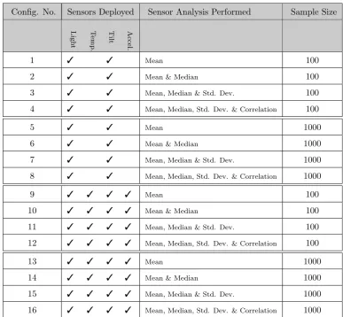
4.3.3 Application Configurations . . . 134
4.3.3.1 Normal Operation . . . 136
0
Chapter 5 Evaluation 141
5.1 Off-line execution using benchmark measurements. . . 144
5.2 Analysis Setup . . . 146
5.2.1 Statistical Analysis Tools . . . 147
5.2.1.1 Independent Two-Sample T-Test . . . 149
5.2.1.2 Non-Parametric Tests . . . 149
5.2.1.3 Correlation Tests . . . 150
5.3 TimePredict Evaluation . . . 150
5.3.1 Software Timeliness . . . 151
5.3.2 TimePredict Performance . . . 154
5.3.3 System Impact . . . 159
5.3.3.1 Timing Overhead . . . 159
5.3.3.2 Memory Consumption . . . 163
5.3.3.3 Power Consumption . . . 166
5.4 Off-line Analysis . . . 168
5.4.1 Comparative Off-line Statistical Analysis . . . 168
5.4.2 Effect of Model Parameters on Predictive Performance . . . 171
5.4.3 Timing Feedback . . . 172
5.5 Summary . . . 173
Chapter 6 Conclusion 174 6.1 Contribution . . . 174
6.2 Future Work . . . 177
6.3 Conclusion . . . 178
Appendix A Software Execution Times 179
List of Tables
2.1 Summary of adaptation approaches. . . 39
2.2 Summary of timing analysis approaches. . . 58
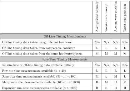
3.1 Effect of measurement availability on timing estimates. . . 65
3.2 Confidence intervals and critical values for the Kolmogorov-Smirnov two-sample test. . . 95
4.1 Available clock speeds and maximum durations on the Java Sun SPOT mote. . . 115
4.2 Execution times of the software benchmark suite, over 20 configurations. . . 128
4.3 Configurations of the sensor software. . . 135
5.1 Summary of the expected contribution matched to particular evaluations. . . 143
5.2 Off-line analysis performed by TimePredict on benchmark measurements. . . 144
5.3 Evaluation of the execution time of the sensor analysis function. . . 151
5.4 Correlations of configuration setup with execution time analysis. . . 152
5.5 TimePredict forecasting accuracy and precision. . . 155
5.6 Correlation between accuracy/precision and the overall range and IQR. . . 158
5.7 Sensor analysis timeliness with and without TimePredict. . . 162
5.8 Statistical tests for any timing interference due to TimePredict. . . 163
5.9 Memory usage with and without TimePredict. . . 163
5.10 95% confidence intervals for memory overhead of TimePredict. . . 165
List of Figures
1.1 Dynamic software adaptation. . . 3
1.2 Architecture of an idealized dynamically-adaptable component-based system. . . 6
3.1 Timing bounds used to define the execution-time performance of software. . . 62
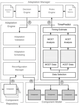
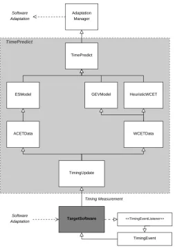
3.2 Architecture of a dynamically-adaptable system featuring TimePredict. . . 69
3.3 Bounded timing estimates using the exponential smoothing model. . . 81
3.4 WCET Heuristic Performance. . . 86
3.5 Gumbel probability distribution. . . 89
3.6 Fr´echet probability distribution. . . 90
3.7 Weibull probability distribution. . . 91
3.8 Pareto probability distribution. . . 92
3.9 Analysis of the difference between Data and Distribution CDFs. . . 94
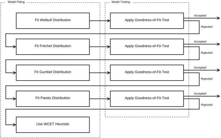
3.10 WCET model fitting process. . . 97
4.1 TimePredict class diagram. . . 102
4.2 Java Sun SPOT mote. . . 105
4.3 Sending a Datagram-based discovery request. . . 107
4.4 Receiving a Datagram, using a blocking receive function. . . 108
4.5 Initializing and using a stream-based connection. . . 109
4.6 Taking sensor readings using the Squawk Java API. . . 110
4.7 Comparison of the System.arraycopy performance. . . 113
4.8 TimingListener interface. . . 119
0
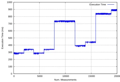
4.10 Execution times for the combined software benchmark functions, over 20,000
mea-surements. . . 126
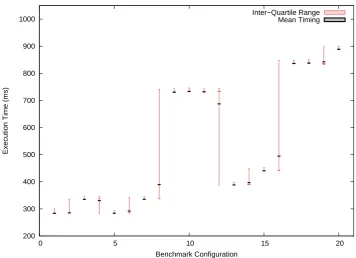
4.11 Boxplot showing the measurements taken of the software benchmark functions, across each of the 20 recorded configurations. . . 129
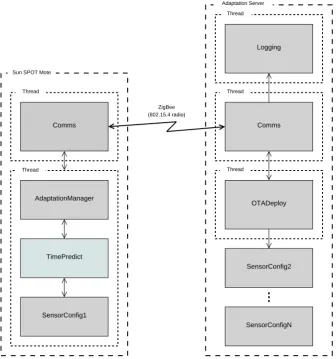
4.12 Experimental setup with Sun SPOT mote and Adaptation Server. . . 132
4.13 Execution order during normal operation. . . 138
4.14 Adaptation request and software deployment. . . 139
5.1 Box-plot showing the maximum and inter-quartile range of execution times. . . . 154
5.2 Histogram of the estimation accuracy of TimePredict. . . 156
5.3 Histogram of the estimation precision of TimePredict. . . 157
5.4 Execution time of the TimePredict functionality on the Sun SPOT mote. . . 160
5.5 Boxplot showing the execution time performance of TimePredict. . . 161
5.6 Boxplot showing the memory consumption of TimePredict. . . 164
5.7 Battery discharge while running software. . . 167
A.1 Detail of the ACET Timing Estimates for Configuration 16, with the red line representing execution time behaviour and the green lines representing the ES estimate bounds. . . 179
A.2 The same timing behaviour for Configuration 16, overlaid with worst-case estimate bounds. . . 180
A.3 Execution Times of Configurations 1 to 4 . . . 181
A.4 Execution Times of Configurations 5 to 8 . . . 182
A.5 Execution Times of Configurations 9 to 12 . . . 183
A.6 Execution Times of Configurations 13 to 16 . . . 184
Chapter 1
Introduction
Ab actu ad posse valet illatio.
From the past one can infer the future.
Latin Maxim
This thesis presents a run-time reactive prediction model to forecast the execution time of
dynamically-adaptable software. The approach taken in this work demonstrates how
highly-variable software execution times can be estimated using using a combination of extreme-value
statistical modelling techniques in parallel with a self-updating Exponential Smoothing model.
Although this thesis deals with run-time software adaptation within embedded devices, the
con-tribution of this work lies not any novel adaptation selection mechanism, but in the estimation
process that can be applied within this unique operating environment. Despite having limited
system resources available, little prior warning of adaptations within the software, and a minimal
period in which to perform the analysis, the composite predictive model described in this thesis
provides a reliable, accurate and precise timing estimate of the changeable execution time of
dynamically-adaptable software.
This chapter introduces the motivation behind this work, and defines the principal ideas
underpinning dynamically-adaptable software. The volatile execution time of this software is
outlined, and the challenges involved in predicting its likely future behaviour are presented.
1.1
Dynamically-Adaptable Software
Software is routinely expected to operate in a correct, reliable and autonomous manner over
prolonged periods without supervision or intervention. This expectation also extends to software
running on resource-constrained devices executing within highly-variable operating environments.
Where there exists a general reluctance to incur any downtime, i.e., where extended periods
of uninterrupted operation are necessary, suspending execution to facilitate software updates
or perform maintenance on the system is not ideal [Oreizy et al., 2008]. This prohibition on
suspending execution mainly serves to restrict the software, once deployed and executing, to a
fixed set of immutable functional behaviours. Unanticipated changes in the environment, or any
unexpected operating conditions, must be handled using this pre-defined functionality. However,
if the functionality remains fixed, and the demands being placed on the software by its operating
environment begin to differ sufficiently from its capabilities, the performance of the system as a
whole can degrade to the point where it becomes unfit for purpose.
To avoid the system becoming periodically unresponsive within such volatile operating
envi-ronments, discrete modifications may be made during execution to optimize the available
func-tionality to the prevailing conditions. Continuously adding hardware to compensate for poor
software performance provides an unrealistic long-term solution, due to high costs, and the
po-tential difficulties in gaining physical access to the system (e.g., as with satellites or embedded
devices). Modifying the software at runtime provides the most practicable means of bridging the
gap between any unanticipated operational challenges, and the apparent limitations of the
sys-tem. By allowing software to adapt itself at run-time, its facility to handle extreme or unexpected
operating conditions is increased, without negatively impacting on its availability.
The Oxford English dictionary defines adaptation as the “the process of modifying a thing so as to suit new conditions” [OED, 1989]. Within the context of software, it is then possible to characterize adaptation as the process of adding, removing or replacing functional elements
within a system to provide a set of behaviours more suited to the current operating environment.
Software adaptations are necessarily reactive processes, in that changes in the operating
envi-ronment occur unexpectedly at run-time and require immediate corrective action in the form of
functional modifications. Changes in the operating environment can take the form of
unantic-ipated events such as device failures or software exceptions, as well as more gradual processes
obsolescence. Software that implements functional adaptations at run-time, i.e., without halting
execution or requiring external intervention, may be described as being dynamically-adaptable.
Buisson et al. define such dynamically-adaptable software as “software that modifies or augments its functionality during execution in response to some observations about its operating environ-ment” [Buisson et al., 2005]. Both the scheduling and the functional scope of adaptations within dynamically-adaptable software are resolved only at run-time, with the principal limitation to
the adaptation process being the availability of suitable alternate functional behaviours.
Fig. 1.1: Dynamic software adaptation.
Figure 1.1 is based upon an illustration of a control loop for self-adaptive systems, originally
described in a survey paper of autonomic software systems [Dobson et al., 2006], and re-produced
here in a slightly modified form. Autonomic, self-adaptive or self-* software are largely analogous
to dynamically-adaptable software in intent, with the slight difference, if it exists at all, being the
added emphasis on unrestricted adaptation within dynamically-adaptable software. Unrestricted
adaptation permits run-time modification of the software in a manner that may not have been
foreseen at design-time. In contrast, autonomic, self-adaptive and self-* software may reasonably
restrict the scope of adaptations to a pre-defined set of alternate functional behaviours, in order
to maintain a desired functional or non-functional property of the system [Keeney, 2004].
There are four broadly defined stages, as illustrated in Figure 1.1, that enable
Analyse,Plan andAdapt. The first stage of an adaptation cycle involves measuring various pa-rameters associated with the performance of the system. This provides information about the
effects of the operating environment on the current configuration of the software, and highlights
any performance deficits should they exist. Continuous measurement of parameters such as the
system load, software interrupts and the overall software execution time allow changes in the
operating environment to be inferred from changes in the measured parameters. The
measure-ment stage facilitates an ongoing assessmeasure-ment of the suitability of the current configuration of
the software. Next, the analysis stage evaluates the various system measurements, and
deter-mines whether firstly, an adaptation is necessary, and secondly, what are the most appropriate
modifications to make to the software. Once this is complete, the planning stage takes the
analysis and constructs an adaptation plan for the system. This plan is based on a
determi-nation of the available alternate software behaviours, their likely functional and non-functional
performance, and the expected difference between these and the performance of the current
con-figuration of the software. Lastly, the adaptation stage takes the completed adaptation plan,
and implements the desired modifications on the executing software, either pausing execution
to effect the adaptation or hot-swapping functional elements at runtime. The timing analysis
approach presented in this thesis, fulfills the analysis role described in Figure 1.1, as well as
enabling the measurement of software timing behaviour. Although the actual implementation
of the adaptation process is largely outside the scope of this work, it is envisaged that the
un-derlying dynamically-adaptable system uses the timing analysis to optimize its execution-time
performance by dynamically adding, replacing or removing functional elements at run-time.
Some software adaptation techniques, e.g., parameter-based adaptation [Sharma et al., 2004],
do not permit any new functional behaviours to be added to the software once the system is
de-ployed. A limited form of adaptation is achieved by altering some existing parameters that govern
the behaviour of the currently deployed software. In contrast, dynamically-adaptable software
takes a less restrictive approach towards the adaptation process, allowing new functionality to be
added much later to the system, at a time dictated by the prevailing operating conditions [Fritsch
and Clarke, 2008]. A number of existing software adaptation techniques support an unrestricted
approach towards run-time functional adaptation, ranging from middleware-based adaptation
schemes [Sharma et al., 2004], to dynamic aspect-weaving frameworks [Assaf and Noy´e, 2008],
frame-works [Zhang et al., 2005].
1.1.1
Component-Based Software
Component-based systems provide the underlying platform for the dynamic software adaptation
considered in this thesis. Software components provide a convenient means of encapsulating
functionality within discrete, composable functional units. Menasc´e defines a software component
as having a well-defined interface, allowing it to be employed in various applications for which
it may or may not have been explicitly designed [Menasc´e et al., 2004]. Szyperski describes a
software component as “a unit of composition with contractually specified interfaces and explicit context dependencies only. A software component can be deployed independently and is subject to third-party composition” [Szyperski and Pfister, 1997]. Software components provide readily accessible units of adaptation, where adapting the software functionality is a matter of simply
changing the components that comprise the system. In this manner, dynamically-adaptable
software can be achieved through adding, replacing or removing software components from the
system at runtime.
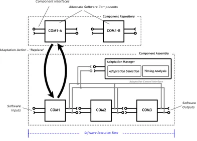
Figure 1.2 presents an idealized dynamically-adaptable component-based system, designed
as a composite of a number of existing run-time adaptation frameworks. These frameworks,
described in more detail in Chapter 2, share the common characteristic of allowing software
to be modified during execution, by adding, removing or replacing discrete functional elements
within the system. The primary focus of this thesis is on predicting the execution time of this
type of dynamically-adaptable system, i.e., a system can add previously unenvisaged functional
behaviours at any stage during its execution. Since the characteristics of the underlying software
will influence the approach used to predict its execution-time behaviour, dynamically-adaptable
systems considered within this thesis are assumed to have the following properties (labelled P1
to P6);
P1: Adaptations are reactive, infrequently occurring events, that modify the functional
be-haviour of software in response to changes in the operating environment.
P2: Adaptations occur unexpectedly during run-time, and are realized within a
dynamically-adaptable system during its normal execution. In order to implement the adaptation, the
system may pause execution briefly to enact the software modification, or alternatively
Fig. 1.2: Architecture of an idealized dynamically-adaptable component-based system.
P3: The functional scope and scheduling of an adaptation cannot be determined at design-time,
and is only resolved at run-time, triggered by changes in its operating environment and
the availability of alternate functionality.
P4: The adaptation process is controlled by a dedicated Adaptation Manager function within
the system. The Adaptation Manager monitors, evaluates, plans and implements
adap-tations automatically at run-time. The goal of the Adaptation Manager is to optimize a
particular property of the dynamically-adaptable system through functional adaptations,
e.g., its execution time.
P5: Adaptations are achieved by adding, replacing or removing one or more software
compo-nents that comprise the system. Software compocompo-nents are discrete units of composition,
that are discoverable and composable at run-time through well-documented interfaces.
discoverable by the Adaptation Manager during run-time. New software components may
be added to this repository at any stage during the execution of the system, and include
software behaviour not originally envisaged at design-time.
A system that exhibits all of these properties may be characterized as being
dynamically-adaptable. For the purposes of this thesis, the primary research question is not about the
nature of dynamically-adaptable systems, nor the adaptation process in itself, but whether a
statistical-based approach, implemented at run-time, can accurately and precisely estimate the
timeliness of a dynamically-adaptable system. In order to illustrate an architecture for an
ide-alized dynamically-adaptable system, and show where within such an architecture the timing
analysis functionality could reside, Figure 1.2 illustrates an adaptable component-based system
formed from three functional components (COM1, COM2 and COM3), as well as one control
component - the adaptation manager. Both service and control interfaces are provided within
each component, in the former case to interface with other components in the assembly, and
in the latter to provide a mechanism for run-time supervision and intervention by the
adapta-tion manager. The execuadapta-tion time of the entire component assembly is measured and recorded
within the adaptation manager, where an analysis of the timeliness of the software forms an
input into the adaptation selection process. An external component repository is provided with
a set of alternate functional behaviours for existing components in the assembly (COM1-A and
COM1-B). In the example, a ‘replace’ adaptation action removes the component COM1 and
inserts COM1-A into the system at run-time under the direction of the adaptation manager.
Software components provide a convenient level of granularity for adaptable systems, since they
can leverage the often highly modularized and localized functionality within a typical codebase
to decompose functional behaviours into discrete units of adaptation. Commonly, high-level
functional behaviours are composed of lower-level functional entities, such as classes, objects or
functions. These functional entities can be encapsulated within an individual software
compo-nent, allowing each component to perform a sub-task within the overall system. Adapting the
software at run-time, i.e., changing the constituent software components within the system, can
be achieved using one of a number of run-time adaptation techniques such as a wrapper pattern,
dynamic linking or middleware re-direction [Salehie and Tahvildari, 2009], however, within the
architecture described in Figure 1.2, software components are hot-swapped into the component
The reactive nature of dynamically-adaptable software requires a dedicated adaptation
man-ager to initiate, select and implement the required functional adaptations, as well as oversee
the general performance of the system. A dedicated internalized adaptation manager can be
encapsulated as a software component, and can execute in parallel with the software,
fulfill-ing the various tasks illustrated in Figure 1.1. For simplicity, and to reduce the complexity of
maintaining a shared system view with an external entity, it is more convenient to co-locate
the adaptation manager component within the component assembly being managed. As well
as managing the functional adaptations to the system, the adaptation manager includes
func-tionality to measure and analyse the execution-time performance of the system. This software
timing analysis is introduced in Section 1.2, and provides an opportune means of accessing the
ongoing fitness of dynamically-adaptable systems, as well as verifying the effects on performance
of run-time software adaptations.
1.2
Software Timeliness
The principal contribution of the work described in this thesis is estimating the timeliness of
dynamically-adaptable software. While many other timing analysis methods currently exist
[Li et al., 2007] [Marref and Bernat, 2008] [Wilhelm et al., 2008], none have been applied to
evaluate the execution time of dynamically-adaptable software running within an embedded
operating environment. The execution time of software may be defined as the period required to
process a given task to completion, under normal operating conditions, on a specified hardware
platform [Edgar, 2002]. All software, including statically-defined software operating under ideal
conditions, tends to experience some minor variations in its execution time due the interaction
of a large number of internal and external factors. I/O latencies, hardware interrupts, software
events, available memory, networking issues, device failures, caching policies, execution history
and even the ambient temperature of the processor all contribute to cause fluctuations in the
timing behaviour of the system [Henia et al., 2005]. Accurately predicting the execution time
allows a more efficient use to be made of the available computational resources, informs the
scheduling of software tasks, and provides an on-going qualitative assessment of the performance
of the software [Becker et al., 2006]. Where the software is capable of modifying its functional
behaviour at run-time, its execution time can form both an input into the adaptation process,
system.
Dynamically-adaptable software responds to changes in its operating environment by
chang-ing parts of its functional make-up. However, knowchang-ing whether the operatchang-ing environment has
changed requires the continuous measurement of various system parameters in order to build up
a ‘true’ picture of the current operating conditions. In effect, the status of the operating
environ-ment must be inferred from a limited set of periodic measureenviron-ments. One of the more revealing
properties of a software system is its ongoing execution-time performance, i.e., its timeliness. If
sufficiently large or prolonged deviations from the established execution time are observed, it can
be inferred that the cause for these changes is some underlying factor within the system itself
or within the operating environment. For example, periods of high load on the system, such as
those caused by large numbers of concurrent user requests, can overwhelm the capabilities of
the system and manifest themselves as execution time delays. In this manner the timeliness of a
dynamically-adaptable system can provide an indication of the capability of the software to
per-form its role. Since dynamically-adaptable software also permits the functionality to be modified
as a reaction to changes in the operating environment (e.g., excessive delays), the timeliness of
the software affords a qualitative point of comparison between candidate adaptations, and the
currently deployed software configuration.
1.2.1
Execution-Time Requirements
Any predictive method that provides a reliable, accurate and precise estimate of the timeliness
of dynamically-adaptable software, also provides re-assurance about the software adhering to its
timing requirements. Software can be divided into three broad categories with respect to its
required timing behaviour, i.e.,
• software with no explicit timing requirements
• software with soft timing requirements, and
• software with hard execution-time requirements.
The first category of timing requirements encompasses software that has been developed without
any expectation of how long it will take to execute. Many software applications written today
fall into this category, with the software developer eschewing execution-time considerations,
software forms an unconsidered, and largely ignored, by-product of its execution. In contrast,
the opposite extreme is software with hard execution-time requirements, where strict inviolable
deadlines are placed on the timeliness of the software. These deadlines must be adhered to
over the life-time of the software, regardless of any difficulties imposed by unusual or extreme
operating conditions. Typically employed within critical real-time and embedded systems, e.g.,
flight control systems [Mindell, 2008], hard execution-time requirements force the software to
complete each task within a preset time period. To miss a timing deadline would mean the
catastrophic failure of the system, since the various tasks making up the system have rigid
pre-determined execution schedules. Hard real-time software is not generally amenable to
run-time adaptation, or even repeated off-line modification, due to the lengthy and detailed analysis
required to verify its timeliness after even minor functional modifications [Wilhelm et al., 2008].
Since the first category of software has no use for execution-time analysis, and hard real-time
software effectively prohibits adaptation, the focus of this thesis is on estimating the timeliness
of software with soft execution-time requirements.
Systems with soft execution-time requirements offer a balance between providing deadlines on
the execution-time of the software and tolerating occasional violations of these deadlines under
extreme or unusual operating conditions. Typically, the software timing deadlines are outlined by
the developer in advance, or determined by the system at runtime, and aimed at ensuring software
tasks execute according to pre-defined but moderately flexible timing constraints. Violations of
soft timing deadlines can and do occur under extreme conditions, but only result in a reduction
in the quality of service, rather than a complete failure of the system. For example, within an
IP telephony application, delays in receiving packets result in a reduction in call/voice quality.
Similarly, delays in rendering a frame within gaming applications result only in momentary
periods of frame jitter. Unanticipated or excessive violations of soft execution-time deadlines can
provide the impetus for adapting the underlying software to better suit the prevailing operating
conditions. Timing deadlines offer a threshold against which the system can be measured, and if
found lacking, can provide a performance target for any subsequent adaptations to the software.
Consequently, changes in the software execution time can prompt functional adaptations
within dynamically-adaptable systems. However, adapting the functional behaviour of even a
small part of the software can result in unintentional changes to the execution time of the software
that these modifications do not negatively impact on software timeliness. For
dynamically-adaptable software to provide any assurance of correct operation, i.e., to avoid any time-induced
functional errors, it must be possible both to recognize when to adapt and to quickly predict the
execution time of a newly-adapted software system.
Unfortunately, the combination of software adaptations, as well as general timing
pertur-bations originating in the operating environment, both may contribute to unintentional
alter-ations in the overall execution time of the software. Within closely-coupled systems with soft
execution-time constraints, poorly understood timing behaviour hampers the ability of the
soft-ware to function as expected. Usually, the outputs of one functional element form the inputs of
the next, meaning that small localized delays can quickly propagate through the system
lead-ing to reduced throughput, missed timlead-ing deadlines, or can even precipitate functional errors in
otherwise dependable code. The correct operation of a dynamically-adaptable system relies as
much on reducing uncertainties about its timing behaviour as removing functional errors from
the code.
1.2.2
Predicting Software Execution Times
Timing analysis is the process of evaluating software to produce an estimate of its likely
execution-time within a specific operating environment. Traditionally, timing analysis has been applied to
hard real-time systems, where the timeliness of the software is critical to the correct performance
of the system. Specifically, the timing analysis methods applied to these critical systems are
concerned solely with deriving a worst-case execution time (WCET) estimate for the software,
in order to provide safety guarantees within hard real-time environments, i.e., an assurance
that the software will never exceed any hard timing deadlines [Wilhelm et al., 2008]. These
traditional timing analysis approaches evaluate the software timeliness using one or more static
analysis methods, applied at design-time to a fixed code-base. The software persists in the same
unchanged form after deployment, ensuring the timing estimate remains valid during execution.
The difference between hard real-time systems and dynamically-adaptable software is borne
out in the expectations surrounding their timing behaviour. The former is expected to remain
fixed once deployed and executing, while the latter is liable to change unexpectedly during
exe-cution, and continue execution with a conspicuously altered execution-time behaviour. The
dynamically-adaptable software. The functional scope of the code is not fixed, and since execution continues
immediately following an adaptation, there is no opportunity to submit the software for extended
periods of off-line testing supervised by a domain expert, i.e., the programmer/developer/tester.
The execution time of dynamically-adaptable software will vary considerably, and change
with-out prior warning. As a result, software adaptations can quickly lead to a divergence between
any static pre-compiled execution-time estimate and the observed execution-time behaviour.
Static timing analysis methods, i.e., those that form an off-line estimate of software
timeli-ness, are insufficient for dynamically-adaptable software since its timing behaviour changes with
every adaptation. Statically analyzing each potential configuration of a dynamically-adaptable
system, similar to the approach described in the PECT framework [Hissam et al., 2003], becomes
impractical when the number of potential configurations of the system grows very large. To
pro-vide an unrestricted framework for dynamic software adaptation, but yet support the prediction
of its execution-time behaviour, software timing analysis must be performed concurrently with
the normal operation of the system and continuously update as the timing behaviour of the
system changes.
Dynamic timing analysis methods currently exist, such as those measurement-based
tech-niques described by Petters [Petters et al., 2007] and Hansen [Hansen et al., 2009], however
they require a large number of timing measurements before an estimate of the timing behaviour
of the software can be created. Since adaptations change the functionality of the system, any
timing measurements recorded prior to an adaptation are invalidated once the software changes.
This requires a new set of timing measurements to be created before a timing estimate can be
produced, potentially leading to a period immediately following an adaptation, where no timing
estimates can be provided. In any dynamically adaptable system the most pressing need for an
estimate of the execution time will be immediately after the system adapts, in order to establish
the performance of the new configuration of the software.
Using statistical models, an accurate estimate of the timeliness of dynamically-adaptable
software can be created. However, statistical models require a set of measurements to fit a selected
statistical distribution to the underlying data, and then produce a valid estimate. Unfortunately,
this minimum number of measurements can range from several dozen to thousands, depending
on the inherent variability in the process being measured, i.e., the software timeliness. The
different statistical analysis techniques to provide an immediate, progressively improving estimate
of the timeliness of dynamically-adaptable software.
Two aspects of the timing behaviour of the dynamically-adaptable software are analyzed, the
average-case timing, and the worst-case execution time. The average-case timing estimate
pro-vides a bounded interval within which a stated percentage of the software timing measurements
are expected to fall. The worst-case estimate provides a single threshold value below which
another stated percentage of the timing measurements of the system are expected to occur.
These two estimates provide an indication of the central tendency of the software execution-time
performance and its potential for extreme behaviour, i.e., timing delays.
A linear regression analysis is applied in the first case, to supply a bounded average-case
timing estimate. For the worst-case performance, a modified Holt-Winters exponential smoothing
model [Chatfield, 2003] is applied initially when a small number of timing measurements are
available, e.g., immediately succeeding an adaptation. The Holt-Winters model is applied to time
series data, in this instance the series of software timing measurements recorded at run-time, and
used to forecast the likely worst-case execution time of the dynamically adaptable software. When
a sufficient number of timing measurements have been recorded, the worst-case timing estimate
is generated using a statistical distribution that is fitted to the timing data at run-time. The class
of statistical distribution used is known as an extreme-value distribution [Kotz and Nadarajah,
2000], and is more usually found in predicting the movement of financial markets [Poon et al.,
2004] or in estimating extreme events [Alvarado et al., 1998].
These statistical modelling techniques, the collection and assimilation of timing measurements
as well as the application of run-time adaptive statistical models to dynamically-adaptable
soft-ware systems, are described in more detail in Chapter 3.
1.2.3
Challenges
In contrast to statically-defined software, dynamically-adaptable systems provide a flexible
frame-work in which developers can create malleable code capable of contending with, and exploiting,
highly variable operating environments. However, run-time adaptations change the timing
be-haviour of the software, and introduce uncertainties about its timeliness that cannot be easily
analysed or predicted in the short period available during or immediately following an
analysis process must either account for every potential configuration of the software statically
(an unrealistic prospect), or perform the analysis at run-time and automatically update the
tim-ing estimate when a functional adaptation occurs. The research question central to this thesis is
how statistically-based timing analysis methods can be applied to dynamically-adaptable
soft-ware at run-time, without halting the system or restricting the number of potential adaptations
to the software.
As the scope and scheduling of adaptations are resolved only at run-time, any estimates
of software timeliness must be capable of rapidly reacting to adaptations within the system.
However, since it is unlikely that any prior timing analysis will have been performed on a new
configuration of the system, the timing analysis process must refresh its estimates using
what-ever timing information is available immediately following an adaptation. This raises a secondary
research question for this work, concerning how an accurate, precise timing estimate may be
pro-duced, when the predictive model is based upon a limited set of timing measurements, recorded
immediately following a software adaptation. From the sparse timing information available an
estimate must then be created without interfering with the normal execution of the software, or
negatively impacting on the functional behaviour of the system. Lastly, since the timing
esti-mate is provided as feedback into the adaptation process, the predictive model used to generate
the estimates must be capable of uncovering subtle changes in software timing behaviour over
extended periods.
1.3
Contribution
This thesis describes the design and evaluation of an execution-time forecasting method for
dynamically-adaptable software. Specifically, the approach presented in this work predicts the
timeliness of software executing on a resource-constrained embedded device with soft real-time
constraints. Timing predictions are generated using reactive run-time statistical methods, and
are continually updated with fresh timing measurements during run-time. The contribution
of this work is therefore in applying novel statistical techniques to estimate the timeliness of
dynamically-adaptable software. Not only that, but to perform this analysis at run-time, within
the same embedded system that is being monitored. This task is made difficult by the unique
nature of the software, as well as the restrictions imposed by the operating environment.
timeliness of the software in unexpected ways. The core of this thesis is a predictive model that
accurately and precisely estimates software timeliness, without halting the system to perform
the analysis, relying on any prior off-line testing or restricting the scope of functional
adapta-tions. Currently, various measurement-based [Colmenares et al., 2008] [Wenzel et al., 2005], and
statistical-based [Hansen et al., 2009] [Edgar, 2002] timing analysis techniques exist, however they
both perform the timing analysis from an off-line context, and preclude any modifications to the
underlying software at run-time. The few autonomic approaches that monitor the performance of
software in real-time and adjust any QoS or performance estimates appropriately [Epifani et al.,
2009] [Calinescu and Kwiatkowska, 2009], likewise do not support any timing analysis where the
underlying software is dynamically adaptable. There is a gap in the current knowledge about
how best to estimate the execution time of software that can both change unexpectedly during
run-time, as well as modify its functionality into a configuration that may be unenvisaged at
design-time.
Timing estimates are produced automatically at run-time using this predictive model, with an
accuracy only slightly below what would be achieved using an industry-standard timing analysis
process performed off-line in ideal circumstances and under manual supervision. In addition to
providing timing estimates of the software, the outputs of this predictive model provide feedback
into the adaptation process as a means of selecting the most appropriate configuration of the
software for the prevailing operating conditions. Lastly, the predictive model, while interleaved
with the normal execution of the software, does not negatively impact the performance of the
system.
1.4
Assumptions
This thesis is grounded in a number of underlying assumptions concerning the overall approach,
the performance of the execution-time forecasting process and its evaluation. In addition, there
are also several fundamental assumptions about the implementation of dynamically-adaptable
software, the nature of the operating environment and the limitations of the adaptation process.
Hardware: The operating environment includes both the hardware running the dynamically-adaptable software system, as well as any external factors that influence software behaviour,
processor(s), memory and storage, all located on the same physical unit. For the purposes of
this thesis, resource-constrained embedded devices provide the target hardware environment,
typically having MHz-scale processors with solid-state memory/storage not in excess of several
hundred megabytes. The use of resource-constrained embedded devices is desirable since it
provides a convenient motivation for application domains where both computing resources and
execution time performance are critical. However, the implication of using resource-constrained
devices is that the forecasting process must minimize both its memory footprint and processing
overhead on the device. In addition, the limited memory cannot store a very large set of timing
measurements, so the forecasting process must selectively store or discard timing data according
to its freshness and/or its descriptive value, i.e., excessive execution times are more useful in
calculating the likely worst-case execution time of the system, than more average measurements.
Rarely Occurring Events: The system is composed of dynamically-adaptable component-based software, and includes an internal adaptation manager with timing analysis functionality.
Adap-tations are assumed to be rarely occurring events, implemented at run-time by changing the
composition of the component-based system, using a set of alternate software components
pro-vided within a component repository. An adaptation process that is called too frequently will
impact on the normal execution of the software, since resources and time will be required to
se-lect and implement changes to the software. For a dynamically-adaptable system to optimize its
functional response, minor variations within its operating environment must be overlooked, and
adaptations triggered only when absolutely required. An overly reactive adaptation process may
potentially create a repeating oscillation between two extreme behaviours, to the detriment of its
functional goals. For a timing analysis process, estimating the execution time of a
dynamically-adaptable system will require some distinct periods of time between adaptation events, where
the timeliness of the system can be appraised, and estimated within a single configuration of the
system. Also, since the measure of a timing analysis process will be its accuracy and precision, a
reasonably stable configuration of the system is required to assess the estimate against observed
behaviour.
dynamically-adaptable software, and to a lesser extent the adaptation process itself, are secondary to the
task of estimating the volatile execution-time behaviour of dynamically-adaptable systems. The
restriction on allowing only stateless components within the adaptation framework is more on
simplifying the adaptation process, since the fact that the software changes at run-time (along
with its execution time), is more critical than the nature of any state management during
adap-tations. If an adaptation framework is introduced to manage state transition between software
components at run-time, there should be no impact on the timing analysis of that
adaptable system. The limitation on using only stateless components within a
dynamically-adaptable system is solely a means of expediting the adaptation process, and in turn
demon-strating the run-time timing analysis approach that forms the subject of this thesis.
Statistical Estimates: The overall approach towards predicting software timeliness uses a statistical-based predictive model, that is generated and updated at run-time, using timing measurements
of the underlying system. The output of this predictive model in turn feeds back into a basic
adaptation selection process, providing an example of one type of input into what could be a
more expansive adaptation selection mechanism. Adaptations, and the adaptation management
process, are limited to functional changes within a single software system. This thesis does not
cover the timing analysis of any adaptations across a distributed environment, nor is there any
provision for forecasting the timeliness of multiple virtual instances of a dynamically-adaptable
software system operating on a single server.
Clock Resolution: The standard system clocks used in this thesis to measure the software exe-cution times are assumed to have a clock resolution on the order of 1 millisecond, meaning that
the error associated with any measurement is assumed to be no more than±1 millisecond. The predictive model in turn, takes these measurements as the basis for its timing estimation process,
assuming that the inherent error in the measurements is negligible compared to the size of the
timing intervals being measured. For applications with a sub-millisecond timing requirement,
the approach outlined in the thesis would still be applicable, but the hardware used to generate
the timing measurements would need to be more fine grained.
execution time of the software will vary between adaptations, as well as over extended periods
of operation within a single configuration of the system, i.e., due to trends in the operating
environment. The predictive model used to generate the timing estimates is assumed to execute
concurrently with the software, be updated regularly, and notified by the adaptation manager
whenever a functional adaptation occurs. The time interval being estimated by this predictive
model is assumed to be the execution of the main control loop of the software, i.e., there is an
underlying assumption that the execution path of the software is cyclical, and comparisons can
be made between individual cycles. Fixing the scope of the analysis to the entire system, rather
than just a sub-component, provides a more relevant assessment of overall performance, and
more readily usable input into the adaptation process.
1.5
Issues Not Covered
The research question at the center of this work is how to accurately estimate the timeliness
of software liable to undergo functional changes at unpredictable intervals. The
dynamically-adaptable software serves only as a framework to demonstrate the predictive model outlined in
this thesis. Specifically, any adaptation selection mechanism, or any other method of evaluating
the optimal configuration of a dynamically-adaptable system at any given time is outside the
scope of this work. Likewise, the scheduling of adaptations or any feature checking associated
with the adaptation process is not considered within this thesis. Adaptations are assumed to
occur rarely, and no provision is made in this work to restrict adaptation cycles from developing,
nor perform any functional analysis on the adaptations themselves.
Similarly, there is no provision in this work for managing any translation of state information
between software components being swapped into the system at adaptation-time. The
implemen-tation of any complex adapimplemen-tation selection process is outside the scope of this thesis, excepting
the assumptions described in Section 1.4. Finally, the determination of the optimal configuration
of the system is not considered in itself, but only as a means of demonstrating timing feedback
1.6
Evaluation
The run-time statistical forecasting approach described in this thesis is required to provide a
precise, accurate estimate of the timeliness of dynamically-adaptable software, without halting
the execution of the system, relying on any detailed off-line analysis, or restricting the scope of
potential adaptations. The accuracy and precision of the timing estimates produced must be
sufficiently reliable and practical to enable an ongoing appraisal of the performance of the system
when compared to its timing requirements. In addition to providing a qualitative assessment of
the performance of the dynamically-adaptable software, the outputs of the timing analysis should
inform the adaptation process, allowing pre-emptive adaptations when the software execution
time is predicted to exceed a set threshold.
An evaluation of the approach outlined in this work must show how accurate execution-time
estimates can be generated, at run-time, in parallel with the normal operation of a
dynamically-adaptable system. The performance of the hybrid statistical forecasting approach is evaluated
using a number of simulated timing behaviours, and then experimentally validated on a
resource-constrained embedded device executing a time-optimizing dynamically-adaptable system. These
latter timing estimates are in turn compared against the outputs of an industry-standard timing
analysis tool, evaluating individual configurations of the software under ideal off-line analysis
conditions.
1.7
Road Map
The remainder of this thesis is structured as follows,
Chapter 2 presents the state of the art in software timing analysis, introduces several time-predictable software design methods, and describes a number of current approaches towards
enabling dynamically-adaptable software.
Chapter 3presents the statistical approach used to forecast the execution-time performance of dynamically-adaptable software. The changeable execution-time performance of this software is
described, and the methods used to generate a run-time predictive model are presented.
Chapter 4presents the implementation of the predictive model.
includes both a number of simulated execution-time traces, and experimental validation using
dynamically-adaptable software executing on a resource-constrained device.
Chapter 6concludes the thesis and discusses potential future work.
1.8
Summary
This chapter has introduced the fundamental concepts behind dynamically-adaptable software
systems, the motivation behind their usage, and the volatile nature of their execution time. The
way in which the execution time of the software both influences the adaptation process, as well
as validates the performance of newly adapted software has been presented.
Since the execution time of the software forms an integral part of both performance
assess-ment and adaptation selection, this chapter described how a predictive process is needed to form
accurate, precise timing estimates without halting the system or restricting the scope of
adap-tations. Lastly, this chapter finishes by describing the contribution of the work, the challenges
Chapter 2
Related Work
In the practical world of computing, it is rather uncommon that a program, once it performs correctly and satisfactorily, remains unchanged forever.
Niklaus Wirth
On the 5th February 1971, astronauts Alan Shepard and Ed Mitchell were preparing to begin their descent towards the surface of the Moon, when an unanticipated software problem prompted
what was possibly one of the first instances of run-time adaptation. Controlling their spacecraft
through its descent and landing was the on-board Apollo Guidance Computer, a weighty device
containing just 2Kb RAM with a 2MHz processing cycle. This early computer system included
various navigational software functions that were manually triggered by the astronauts at
appro-priate moments during the flight. However, the software responsible for guiding them to a safe
landing was exhibiting some worryingly anomalous behaviour and had been noticed both by the
astronauts themselves and the ground controllers monitoring the spacecraft telemetry.
Unknown to the astronauts, a tiny piece of solder, used to attach internal wiring to a switch
on the spacecraft console, had become loose and was periodically setting and resetting an abort
indicator bit within a memory register. If this spurious abort signal was to occur at a critical
point during the descent, the software would automatically override the pilot, and move the
craft into a safe orbit, effectively ending any possibility of a landing. A software fix was required
that would both command the system to ignore any spurious abort signals as well as integrate
and the planning of a suitable adaptation to the software, had to be carried out remotely by
ground controllers, and then forwarded to the astronauts to be manually keyed into the system
to implement the desired change. To further complicate matters, the window of opportunity for
the landing meant the software fix needed to be in place within two hours of the first detection
of the error.
The process that was followed, and the eventual bit-level software adaptation that was
imple-mented, is described in greater detail by Mindell [Mindell, 2008], and provides a microcosm of the
software adaptation process introduced in Chapter 1. Timely analysis, albeit by a large number
of experts already familiar with the system, coupled with remote testing on duplicate hardware
and a robust design of the software, enabled a safe resolution of the error and a successful
land-ing. Unfortunately, with the increasing complexity and responsibility of adaptable systems, the
ability of a human-in-the-loop to both analyze and plan software adaptations has become more
difficult, especially when the deadline on performing an adaptation is often now measured in
milliseconds rather than hours [Smits et al., 2009]. Due to this time-pressure, adaptable
soft-ware frameworks must often implement functional changes without waiting for the approval of
software developer, or without any apriori testing on duplicate systems. Where there are a very
large number of potential adaptations to system, an exhaustive static analysis of each software
configuration may prove impractical. Conversely, run-time analysis is hampered by the software
changing unexpectedly and with limited prior warning, as well as having only a short period in
which to conduct any testing.
The principal contribution of this thesis is a method to automatically estimate the execution
time of dynamically-adaptable software, without restricting the functional scope of any
adapta-tions or halting and restarting the system to perform the analysis. Consequently, the main body
of related work described in this chapter concerns the current state of the art in software
tim-ing analysis, with an emphasis on timtim-ing analysis methods applicable to dynamically-adaptable
software systems. An overview of the various software adaptation frameworks is presented first,
describing the ways in which adaptations may be applied to software at various stages during its
design, implementation and execution. This chapter then concludes with a summary of current
adaptation techniques as well as timing analysis methods, and discusses the approaches that
2.1
Software Adaptation
Software adaptation can be defined as the modification of software to suit new operating
con-ditions. A number of adaptation frameworks currently exist, that support diverse approaches
towards the design, scheduling, implementation and modification of adaptable software systems.
For the purposes of this thesis, the goal of the run-time adaptation process is to optimize the
execution-time performance of the software under a range of operating conditions. For
exam-ple, if the system starts to exhibit a significant delay in processing tasks during periods of high
load, processor-intensive software components are automatically replaced by lightweight
alterna-tives. Within the idealized dynamically-adaptable system, introduced in the previous chapter,
the adaptation process would either briefly pause execution, or hot-swap components at
run-time to effect the desired functional changes. However, different adaptation frameworks each
impose a slightly different set of limitations on the adaptation process, such as restrictions on
when adaptations can occur and what constraints must be applied to the design of the
under-lying software. In order to characterize these different approaches towards software adaptation,
this section evaluates current adaptation frameworks according to six basic questions
concern-ing their motivation, focus, scope, schedulconcern-ing, autonomy and implementation. These questions,
initially outlined by Salehie and Tahvildari [Salehie and Tahvildari, 2009], are expanded below,
and summarized as follows;
- Why are software adaptations required?
The primary motivation behind software adaptations are unexpected changes in the
oper-ating environment. However, the impetus for other adaptation frameworks may include a
number of functional, non-functional or system-specific issues, depending on the
require-ments of the system or the nature of the operating environment. Functional concerns
include scheduled upgrades, run-time patches and event-driven functional updates
[Or-eizy et al., 2008]. Non-functional concerns encompass perceived deficiencies in the
per-formance of the system not directly related to its functionality, e.g., the processor load,
memory footprint or execution time, that necessitate corrective action in the form of a
software adaptation [Sharma et al., 2004]. Lastly, system-specific issues prioritize a
par-ticular facet of the software for adaptation in order to preserve a dominant property of
the system, e.g., adapting the software to resolve security concerns [Perkins et al., 2009],
reliability issues within highly-available systems [Zhang et al., 2005]. In contrast to the
type of unconstrained dynamic software adaptation that forms the primary focus of this
thesis, system-specific adaptation frameworks restrict adaptations to achieve more limited
aims, e.g., improving system security against network-based attacks [Chess et al., 2003].
Unconstrained dynamically-adaptable systems may change the objective function driving
the adaptation process during execution, e.g., initially adapting the software to improve
timeliness, followed by subsequent adaptations to improve its memory usage.
- Where does the adaptation take effect?
Software adaptations can target different logical layers within the system, depending on the
adaptation framework being used. Adaptations may be applied to software at a per
pro-cess, per component, per class, per function or per function-call level. Typically however,
adaptation frameworks limit the scope of an adaptation action to a single layer within the
system, enacting functional modifications on that layer alone. For example,
component-based adaptation frameworks assume that any functional changes are restricted to the level
of components [Ayed and Berbers, 2007], i.e., adaptation actions are implemented through
the addition, replacement or removal of individual software components within the system.
Other interpretations on where adaptations can take effect include dynamically creating
processes within adaptive grid-based systems [Buisson et al., 2007], restricting adaptations
to an adaptive middleware layer [Sharma et al., 2004], or intercepting and re-directing
method calls [Assaf and Noy´e, 2008]. In this chapter, the question of where adaptations
occur within the system is used to categorize the various approaches and frameworks that
facilitate software adaptation.
- What is the result of an adaptation?
Adaptation frameworks may be grouped according to the extent of the functional change
each adaptation can have on the underlying software. Functional modifications may
dis-cretely alter existing software behaviour or may, alternatively, replace entire parts of the
system with new, updated or alternate functionality. Static composition is the most
re-strictive form of adaptation, since execution must be halted to implement what effectively
amounts to a re-design of the system carried out off-line [Hissam et al., 2003].
Parameter-based adaptation permits limited modifications to the software at run-time [Ensink et al.,