Implicit-Explicit Time Stepping Scheme Based on
the Streamline Diffusion Method for Fluid-fluid
Interaction Problems
Lingzhi Qian, and Huiping Cai
∗Abstract—In this paper, we study numerical approximations for the fluid-fluid interaction problems. As a simplified model, the convection-dominated convection-diffusion-reaction equa-tions are coupled by an interface condition. The implicit-explicit time stepping streamline diffusion method for the problem is proposed. The stability analysis and error estimates for the proposed scheme are derived. Computational tests are performed to demonstrate the robustness of this scheme.
Index Terms—fluid-fluid interaction problems, implicit-explicit method, streamline diffusion, stability analysis, error estimates.
I. INTRODUCTION
T
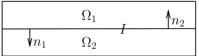
HERE are many problems in which different physical models, different parameter regimes, or different so-lution behaviors are coupled across interfaces. Monolithic solution methods for solving the coupled problems are alter-native. But these methods preclude usage of highly optimized black box subdomain solvers. Decoupling methods have obvious and large advantages in these aspects over mono-lithic solution methods. Among these decoupling methods, partitioned time stepping scheme is promising for solving the coupled problems. In this scheme, a convenient decoupling strategy for large problems is provided. At each time step, we solve the coupled problems by passing information across interface, then the coupled problems are decoupled into individual subproblems independently. Typical applications in which the partitioned time stepping scheme is highly desirable include atmosphere-ocean coupling and fluid-solid interaction problems [3], [4], [5].In this paper, we consider a simplified model of two convection-diffusion equations coupled across their common interface through a jump condition. This reduced problem still retains the essential difficulty of the coupled problems. Fig. 1 illustrates the subdomains considered here, and the domain consists of two subdomains Ω1 and Ω2 coupled
across an interface I = ∂Ω1 ∩∂Ω2, where Ωi ⊂ R2 is
Manuscript received October 09, 2017; revised 20 April, 2018; revised second 23 May, 2018. This work was supported in part by the Jiangsu Key Laboratory for Numerical Simulation of Large Scale Complex Systems open funded projects (No. 201701), Scientific research starting foundation for the high level talents of shihezi university (No. RCSX201732) and Independent-ly funded research projects of Shihezi university (No. ZZZC201751B).
Lingzhi Qian is with Department of Mathematics, College of Sciences, Shihezi University, Shihezi 832003, P.R. China; the Jiangsu Key Labo-ratory for NSLSCS, School of Mathematical Sciences, Nanjing Normal University, Nanjing 210023, P.R. China; College of Mathematics and System Sciences, Xinjiang University, Urumqi 830046, P.R. China e-mail: [email protected].
∗Corresponding author: Huiping Cai is with the Department of
Mathe-matics, College of Sciences, Shihezi University, Shihezi 832003, P.R. China e-mail:[email protected].
a bounded domain with piecewise smooth boundary ∂Ωi. We set Γi = ∂Ωi\I, for i = 1,2. The problem studied in this paper is: given µi > 0 (i=1,2), k ∈ R, find ui: Ωi×[0, T]→R satisfying
ui,t−µi∆ui+β⃗i(x, t)· ∇ui+σi(x, t)ui=fi inΩi, −µi∇ui·⃗ni =k(ui−uj) onI, i, j= 1,2, i̸=j, ui(x,0) =u0i(x) in Ωi,
ui= 0 onΓi,
(1)
where ui,t = ∂u∂ti, β⃗i(x, t) ∈ L∞(0, T;W1,∞(Ωi)) and σi(x, t)∈L∞(0, T;L∞(Ωi)),µi ≪ |β⃗i|=
√
β2
i1+β 2
i2. In
the following, it is assumed that there is a positive constant
γ0 such that
0< γ0≤σi(x, t)−
1 2div
⃗
βi(x, t) ∀(x, t)∈Ωi×[0, T].
This is a standard assumption in the analysis of the problem (1).
Denote Qi = Ωi ×[0, T], b0 = max
i supQ
i
|β⃗
i(x, t)|,
b1 = max
i ||div ⃗
βi(x, t)||L∞(Qi), µ0 = min{µ1, µ2}, σ0 = max
i ||σi(x, t)||L∞(Qi). Let Xi := {
vi ∈ H1(Ωi) : vi =
0 on Γi }
. For ui ∈ Xi, set u = (u1, u2) and X :=
{
(v1, v2) :vi∈H1(Ωi) :vi= 0onΓi, i= 1,2 }
. A natural subdomain variational formulation for the problem (1) is to find (fori, j= 1,2, i̸=j )ui: [0, T]→Xi satisfying
(ui,t, vi)Ωi+µi(∇ui,∇vi)Ωi+
∫
I
k(ui−uj)vids
+(β⃗i· ∇ui, vi)Ωi+ (σiui, vi)Ωi= (fi, vi)Ωi, (2)
for allvi ∈Xi. The natural monolithic variational formula-tion for (1) is to findu: [0, T]→X satisfying
(ut,v) +µ(∇u,∇v) + ∫
I
k[u][v]ds+ (β⃗· ∇u,v)
+(σu,v) = (f,v), (3)
for allv∈X, where[·]denotes the jump across the interface
I,(·,·)is theL2(Ω1∪Ω2)inner product andµ=µi, f=fi inΩi.
It is well known that dominating convection feature has a hyperbolic nature. Standard applications of the finite element method to convection-dominated problems usually lead to unstable numerical schemes. To overcome these difficulties, some modified nonstandard finite element methods can be used such as the streamline diffusion (SD) method [10], [13], [14], [15], [16], [17]. The SD method has both stability
IAENG International Journal of Applied Mathematics, 48:3, IJAM_48_3_06
n
1
n
2
Ω
1
Ω
2
[image:2.595.139.461.80.171.2]I
Fig. 1: Example adjoining subdomains
properties and higher accuracy. For time-dependent problem-s, we use the SD finite element method discrete only in space variables and the finite difference discrete in time direction [12], [21], [22]. This method keeps the essential aspect of the original SD method and simplifies the algorithm structure [1], [6], [8], [9], [18], [20], [23], [24].
In this paper, an implicit-explicit time stepping scheme based on the SD method is proposed for the two domain convection-dominated convection-diffusion-reaction problem. The natural combination of partitioned implicit-explicit time stepping scheme with the SD method retains the best features of both methods, then the proposed method has a number of attractive computational properties for this problem: stable convergence, convenience to decouple large problems, easy implementation of subdomain solvers, parallel computation in decoupled subdomain equations. The stability analysis and error estimates of the proposed method are developed. Finally, some numerical experiments are given to compare this new scheme with the standard implicit-explicit time stepping scheme for this problem.
The remainder of this work is organized as follows: in Section 2, the implicit-explicit time stepping algorithm is described. Stability analysis of the proposed method is presented in Section 3. Convergence results of the proposed method are provided in Section 4, and computations are performed to investigate stability and accuracy of this new algorithm in Section 5. Finally, Section 6 presents the con-clusions and future research directions.
II. PRELIMINARIES
SetL2(Ω) =L2(Ω
1)×L2(Ω2). Foru, v∈X, define the
L2 inner product
(u,v) = ∑
i=1,2
∫
Ωi
uividx,
and theH1 inner product
(u,v)X= ∑
i=1,2 (
∫
Ωi
uividx+ ∫
Ωi
∇ui· ∇vidx),
and the induced norms ||v|| = (v,v)12, and ||v||X =
(v,v)
1 2 X.
LetTibe a triangulation ofΩi andTh=T1∪T2,hbe the
mesh parameter ofThand0< h≤h0<1. TakeXi,h⊂Xi
to be conforming finite element spaces for i = 1, 2, and defineXh=X1,h×X2,h⊂X. It follows thatXh⊂X is a Hilbert space with corresponding inner product and induced norm. Foru∈X, we define the operatorsA, B:X→(X)′
via the Riesz representation theorem as
(Au,v) = ∑
i=1,2
µi ∫
Ωi
∇ui· ∇vidx ∀v ∈X, (4)
(Bu,v) =k
∫
I
[u][v]ds ∀v∈X. (5)
The discrete operatorsAh, Bh :Xh →(Xh)
′
=Xh are defined analogously by restricting (4) and (5) tovh∈Xh.
The partitioned time stepping scheme based on the SD method can be stated as follows: findui: [0, T]→Xi, such that
(ui,t, vi+δviβi⃗ )Ωi+µi(∇ui,∇vi)Ωi
+
∫
I
k(ui−uj)vids−µi(∆ui, δvi⃗βi)Ωi (6)
+ (uβ⃗i+σiui, vi+δvi⃗βi)Ωi = (fi, vi+δvi⃗βi)Ωi,∀vi∈Xi,
where viβi⃗
△
= β⃗i· ∇vi and δ > 0 is an appropriate artifi-cial diffusion parameter. We propose the following choice: restricting∆t≤ahand taking
δ=
{
δ1=a1∆t, if µb0
0 ≤h≤h0,
δ2=a2∆t2, ifh < µb0
0,
(7)
herea1anda2 are two positive constants. The choice fora1
anda2 will be specified in Theorem 3.1. The corresponding
monolithic variational formulation is to findu: [0, T]→X
satisfying
(ut,v+δv⃗β) + (Au,v) + (Bu,v)−µ(∆u, δvβ⃗)
+ (uβ⃗+σu,v+δvβ⃗) = (f,v+δv⃗β)∀v∈X. (8)
Now the implicit-explicit time stepping scheme based on the SD method is stated as follows:
Let ∆t > 0, for each M ∈ N, M ≤ T
∆t, given u
n ∈
Xh, n= 0, 1,· · · , M−1, findun+1∈Xh satisfying
(u
n+1−un
∆t ,v+δv⃗β) + (Ahu n+1
,v) + (Bhun,v)
−µ(∆un+1, δvβ⃗) + (unβ⃗+1+σu
n+1,v+δv
⃗
β) (9)
= (f(tn+1),v+δvβ⃗), ∀ v∈Xh.
IAENG International Journal of Applied Mathematics, 48:3, IJAM_48_3_06
In order to analysis the stability and convergence, it is necessary to work with norms induced by the operators A
andB and relate these norms to || · || and|| · ||X.
Lemma 2.1: [7] Letv= (v1, v2)∈X andα≥0. Then
||v||A+αI =
{ ∑
i=1,2
µi ∫
Ωi
|∇vi|2dx+α
∑
i=1,2
∫
Ωi
|vi|2dx
}1/2
(10)
defines a norm on X. Furthermore, there exists a constant
C >0 such that ifα∈R+ satisfies
α≥Ck2max{µ1−1, µ−21}, (11)
then it follows that
||v||A+αI−B =
{ ∑
i=1,2
µi ∫
Ωi
|∇vi|2dx
+α∑
i=1,2
∫
Ωi
|vi|2dx−k
∫
I
|v1−v2|2ds
}1/2
(12)
defines a norm on X. The above norms are equivalent to
|| · ||X.
The following discrete Gronwall lemma will also be utilized in the subsequent analysis.
Lemma 2.2: [11] Letl, m, andas, bs, ds, gs, for integers s≥0, be nonnegative numbers such that
an+l n ∑
s=0
bs≤l n ∑
s=0
dsas+l n ∑
s=0
gs+m, ∀n≥0. (13)
Suppose that lds <1 for all s, and set ρs ≡(1−lds)−1. Then
an+l n ∑
s=0
bs
≤exp
(
l n ∑
s=0
ρsds ){
l n ∑
s=0
gs+m
}
, ∀n≥0. (14)
III. STABILITY ANALYSIS
In this section, we will give the stability analysis of the presented scheme. Throughout this paper,Cidenotes positive constant independent ofµ, ∆tandh.
Theorem 3.1: Let un+1 ∈ X
h satisfy (9) for each n ∈
{0, 1,· · · ,∆Tt −1}, and 0 < ∆t < (2α+b2
0)−1 for α
satisfying (11). Then there exists nonnegative numbersC1(α)
andC2(α)such that
||un+1||2+ ∆t
n∑+1
k=0
||uk||2X+δ∆t
4
n ∑
k=0
||uk⃗
β||
2
≤C1(α)eC2(α)T
{
||u0||2+ ∆t||u0||2X
+ ∆t n+1
∑
k=0
||f(tk+1)||2
}
. (15)
Proof.Taking v=uk+1 in (9), it follows that
(u
k+1−uk
∆t ,u
k+1+δuk+1
⃗
β ) + (Ahu
k+1,uk+1)
+ (Bhuk,uk+1)−µ(∆uk+1, δukβ⃗+1)
+ (uk⃗+1
β +σu
k+1,uk+1
+δuk⃗+1
β ) = (f(t
k+1),uk+1+δuk+1
⃗
β ). (16)
At first, we estimate the terms of left-hand sides of (16). It is easy to see that
(u
k+1−uk
∆t ,u
k+1)≥ 1 2∆t(||u
k+1||2− ||uk||2), (17)
(u
k+1−uk
∆t , δu k+1
⃗
β ) =
δ
∆t[(u
k+1,uk+1
⃗
β )−(u
k,uk+1
⃗
β )]
≥ −1
2
{
δ
∆tb1||u
k+1||2+ ( δ ∆t)
2||∇uk+1||2+b2 0||u
k||2
}
.
For caseδ=δ1, that is ∆δt =a1, choose a1>0 such that
a21≤µ0 and a1b1≤
1 2γ0.
Ifδ =δ2, then ∆δt =a2∆t andh < µb00, ∆t ≤ah < aµb00,
we can choosea2>0such that
a22a2≤ b
2 0
µ0
and a2ab1
µ0
b0 ≤
1 2γ0.
Then in the above two cases, we have
(u
k+1−uk
∆t , δu k+1
⃗
β )≥ −
1 2
{
µ0||∇uk+1||2
+1 2γ0||u
k+1||2+b2 0||u
k||2
}
. (18)
In addition
(uk⃗+1
β +σ
k+1uk+1,uk+1+δuk+1
⃗
β ) =δ||u k+1
⃗
β ||
2
+ ((σk+1−1
2div
⃗
βk+1)uk+1,uk+1) +δ(σk+1uk+1,uk⃗+1
β )
≥ δ
2||u
k+1
⃗
β ||
2−δ 2σ
2 0||u
k+1||2+γ
0||uk+1||2.
Choosinga1 anda2 again, such that
a1ah0σ20≤ 1
2γ0 and a2a 2(µ0
b0
)2σ20≤ 1
2γ0,
then we have
(uk⃗+1
β +σ
k+1uk+1,uk+1+δuk+1
⃗
β )
≥δ
2||u
k+1
⃗
β ||
2+3 4γ0||u
k+1||2, (19)
and
(µ∆uk+1, δuk⃗+1
β )≤
δ
4||u
k+1
⃗
β ||
2+δµ2C2 0h−
2||∇uk+1||2.
In the caseδ=δ1, we have µb00 ≤h≤h0, choosinga1such
that
aa1h0µ2C02h− 2≤aa
1h0C02b 2 0≤
1 2µ0.
In the case δ =δ2 = a2∆t2 ≤ a2a2h2, choosing a2 >0,
such that
a2a2h2C02h−
2µ2≤ 1 2µ0,
then we get
(µ∆uk+1, δuk⃗+1
β )≤
δ
4||u
k+1
⃗
β ||
2+µ0 2 ||∇u
k+1||2. (20)
IAENG International Journal of Applied Mathematics, 48:3, IJAM_48_3_06
Since δ≤max{a1ah0, a2a2(µb00)2}, combing (16)-(20), we
have
1 2∆t(||u
k+1||2− ||uk||2) + (A
huk+1,uk+1)
+ (Bhuk,uk+1) + δ
4||u
k+1
⃗
β ||
2+γ0 2 ||u
k+1||2−b20 2||u
k||2
= (f(tk+1),uk+1) + (f(tk+1), δuk⃗+1
β )≤
γ0 2||u
k+1||2
+ 1
2γ0||
f(tk+1)||2+δ 8||u
k+1
⃗
β ||
2 +2
δ||f(t k+1
)||2
≤γ0
2||u
k+1||2+δ 8||u
k+1
⃗
β ||
2+C
1||f(tk+1)||2. (21)
Adding α(uk+1,uk+1) to both sides of (21), and applying
Lemma 2.1, it follows
1 2∆t(||u
k+1||2− ||uk||2) +||uk+1||2
A+αI
+ (Bhuk,uk+1) + δ
8||u
k+1
⃗
β ||
2−b20 2||u
k||2
≤C1||f(tk+1)||2+α||uk+1||2. (22)
Note that
(Bhuk,uk+1)
≥ −1
2(Bhu
k+1,uk+1)−1 2(Bhu
k,uk), (23)
combining (12), (22)-(23), we get
1 2∆t(||u
k+1||2− ||uk||2) +1 2||u
k+1||2
A+αI−B
+1 2(||u
k+1||2
A+αI− ||u k||2
A+αI)
+1 2||u
k||2
A+αI−B+ δ
8||u
k+1
⃗
β ||
2≤C
1||f(tk+1)||2
+α||uk+1||2+b 2 0 2||u
k||2.
(24)
Summing over k= 0, 1,· · ·, nfor (24) yields
1 2∆t(||u
n+1||2− ||u0||2) +1 2(||u
n+1||2
A+αI− ||u
0||2
A+αI)
+1 2
n ∑
k=0
(||uk+1||2A+αI−B+||uk||2A+αI−B) +δ 8
n ∑
k=0
||uk⃗+1
β ||
2
≤ n ∑
k=0
(C1||f(tk+1)||2+α||uk+1||2+
b2 0 2||u
k||2). (25)
After multiplying by2∆tand rearranging terms of (25), we obtain
||un+1||2+ ∆t||un+1||2A+αI+ ∆t
n ∑
k=0
(
||uk+1||2A+αI−B
+||uk||2A+αI−B
)
+δ 4∆t
n ∑
k=0
||uk⃗+1
β ||
2
≤ ||u0||2+ ∆t||u0||2A+αI+C1∆t
n ∑
k=0
||f(tk+1)||2
+ (2α+b20)∆t n ∑
k=0
||uk+1||2. (26)
Taking dn ≡ 2α+b20 and using Lemma 2.2 for (26), it
follows that
||un+1||2+ ∆t||un+1||2A+αI+ ∆t
n ∑
k=0
(||uk+1||2A+αI−B
+||uk||2A+αI−B) + δ
4∆t
n ∑
k=0
||uk⃗+1
β ||
2
≤eC2(α)T
{
||u0||2+ ∆t||u0||2A+αI+ ∆t
n ∑
k=0
||f(tk+1)||2
}
,
whereC2(α) = (2α+b20)(1−(2α+b20)∆t)−1. From Lemma
2.1, the norms of|| · ||A+αI and|| · ||A+αI−B are equivalent
to||·||X, we can determineC1(α)and derive the final result.
IV. CONVERGENCE RESULTS
Theorem 4.1: Letu(t;x)∈X for allt∈(0, T)solve the problem (1) such thatut∈ L2(0, T;X) and utt ∈L2(Ω). There exists nonnegative numbersC3(α)andC4(α), for any
n∈ {0, 1,· · ·, T
∆t−1}, and0<∆t <(2α+b
2
0+ 2)−1 for
αsatisfying (11), the solutionun+1∈X
h of (9) satisfies
||u(tn+1)−un+1||2+ ∆t||u(tn+1)−un+1||2X
+∆t 2
n ∑
k=0
||u(tk+1)−uk+1||2X+
δ∆t
12
n ∑
k=0
||uβ⃗(tk+1)−ukβ⃗||2
≤C3(α)eC4(α)T
{
||u(0)−u0||2+ ∆t||u(0)−u0||2X
+ (∆t)2||ut||2L2(0,T;X)+ (4δ+ 1)(∆t)2||utt||2L2(0,T;L2(Ω))
+ inf v0∈X
h
{
||u(0)−v0||2+ ∆t||u(0)−v0||2X
}
+ (12δ+ 1) inf v∈Xh
||(u(0)−v)t||2
+T max
k=0,1,···,n+1vkinf∈Xh||u(t
k)−vk||2
X
+µ2δT max
k=0,1,···,n+1vkinf∈X h
||∆(u(tk)−vk)||2
}
. (27)
Proof.Restricting test functions toXh, subtracting (9) from
(8) yields the error equation
(ut(tk+1)−
uk+1−uk
∆t ,v+δv⃗β)
+ (A(u(tk+1)−uk+1),v) + (B(u(tk+1)−uk),v)
−µ(∆(u(tk+1)−uk+1), δvβ⃗)
+ ((uβ⃗+σu)(tk+1)−(uk⃗+1
β +σ
k+1uk+1),v+δv
⃗ β)
= 0. (28)
Definerk+1=ut(tk+1)−u(t
k+1)−u(tk)
∆t and rearrange terms
(rk+1,v+δvβ⃗)
+ (u(t
k+1)−uk+1
∆t −
u(tk)−uk
∆t ,v+δvβ⃗)
+ (A(u(tk+1)−uk+1),v) + (B(u(tk+1)−uk),v)
−µ(∆(u(tk+1)−uk+1), δvβ⃗) + ((uβ⃗+σu)(t k+1)
−(uk⃗+1
β +σ
k+1uk+1),v+δv
⃗
β) = 0. (29)
Define for each k= 0,1,· · · the functions (u(tk)−vk) + (vk−uk) =ηk+ξk, where vk ∈Xh is arbitrary. Then by
IAENG International Journal of Applied Mathematics, 48:3, IJAM_48_3_06
adding and subtracting vk, (29) may be rewritten as
1 ∆t(ξ
k+1−ξk,v+δv ⃗ β) + (Aξ
k+1,v)
+ (B(u(tk+1)−uk),v)−(µ∆ξk+1, δv⃗β)
=− 1 ∆t(η
k+1−ηk,v+δv ⃗
β)−(Aη k+1,v)
−(rk+1,v+δvβ⃗) +µ(∆ηk+1, δvβ⃗).
−(ηk⃗+1
β +σ
k+1ηk+1,v+δv
⃗
β) (30)
Note that
Bu(tk+1)−Buk =B(u(tk+1)−u(tk)) +Bηk+Bξk,
hence by choosing v=ξk+1, we have
1 ∆t(ξ
k+1−ξk, ξk+1+δξk+1
⃗
β ) + (Aξ
k+1, ξk+1)
+ (Bξk, ξk+1)−(µ∆ξk+1, δξk⃗+1
β )
+ (ξk⃗+1
β +σ
k+1ξk+1, ξk+1+δξk+1
⃗
β )
=− 1 ∆t(η
k+1−ηk, ξk+1+δξk+1
⃗
β )
−(rk+1, ξk+1+δξk⃗+1
β )−(Aη
k+1, ξk+1)
−(ηk⃗+1
β +σ
k+1ηk+1, ξk+1+δξk+1
⃗
β )
+µ(∆ηk+1, δξk⃗+1
β )−(Bη
k, ξk+1)
−(B(u(tk+1)−u(tk)), ξk+1). (31)
The terms on the left-hand side of (31) are bounded below as in the proof of Theorem 3.1. Addingα||ξk+1||2A+αI to both sides, and applying ||ξk+1||2A+α||ξk+1||2 =||ξk+1||2A+αI, it follows
1 2∆t(||ξ
k+1||2− ||ξk||2) +||ξk+1||2
A+αI+ (Bξk, ξk+1)
+δ 4||ξ
k+1
⃗
β ||
2+γ0 2 ||ξ
k+1||2−b 2 0 2||ξ
k||2
≤ − 1
∆t(η
k+1−ηk, ξk+1+δξk+1
⃗
β )
−(rk+1, ξk+1+δξk⃗+1
β )−(Aη
k+1
, ξk+1)
+µ(∆ηk+1, δξk⃗+1
β )−(Bη
k, ξk+1)
−(ηk⃗+1
β +σ
k+1ηk+1, ξk+1+δξk+1
⃗
β )
−(B(u(tk+1)−u(tk)), ξk+1) +α||ξk+1||2. (32)
The error terms involving the operatorBmust be absorbed into theA+αI norms. Using similar technique in Theorem 3.1, we have
1 2∆t(||ξ
k+1||2− ||ξk||2) +1 2||ξ
k+1||2
A+αI−B
+1 2(||ξ
k+1||2
A+αI− ||ξ k||2
A+αI) +
1 2||ξ
k||2
A+αI−B
+δ 4||ξ
k+1
⃗
β ||
2+γ0 2 ||ξ
k+1||2−b20 2||ξ
k||2
≤ − 1
∆t(η
k+1−ηk, ξk+1+δξk+1
⃗
β )−(Aη
k+1, ξk+1)
−(rk+1, ξk+1+δξk⃗+1
β ) +µ(∆η
k+1, δξk+1
⃗
β )
−(ηk⃗+1
β +σ
k+1ηk+1, ξk+1+δξk+1
⃗
β )−(Bη
k, ξk+1)
−(B(u(tk+1)−u(tk)), ξk+1) +α||ξk+1||2. (33)
Now we estimate the terms of the right-hand side in (33), it is easy to see
− 1
∆t(η
k+1−ηk, ξk+1)−(rk+1, ξk+1)
≤1
2||
ηk+1−ηk
∆t ||
2+1 2||r
k+1||2+||ξk+1||2,
− 1
∆t(η
k+1−ηk, δξk+1
⃗
β )−(r
k+1, δξk+1
⃗
β )
≤6δ||η
k+1−ηk
∆t ||
2+ 6δ||rk+1||2+ δ 12||ξ
k+1
⃗
β ||
2,
−(ηk⃗+1
β +σ
k+1ηk+1, ξk+1)
= (ηk+1, ξk+1 ⃗
β )−((σ
k+1−div ⃗βk+1)ηk+1, ξk+1)
≤ δ
24||ξ
k+1
⃗
β ||
2+6
δ||η
k+1||2+C
3||ηk+1||2+
γ0 2 ||ξ
k+1||2,
−(ηk⃗+1
β +σ
k+1ηk+1, δξk+1
⃗
β )≤
δ
24||ξ
k+1
⃗
β ||
2+C
4||ηk+1||2X,
µ(∆ηk+1, δξk⃗+1
β )≤
δ
24||ξ
k+1
⃗
β ||
2+ 6µ2δ||∆ηk+1||2.
The remaining three terms of the right hand in (33) require special treatment. Note that
−(Aηk+1, ξk+1) = ∑
i=1,2
{
µi ∫
Ωi
∇ηik+1· ∇ξik+1dx
}
≤ ∑
i=1,2
µi {∫
Ωi
|∇ηik+1|2dx
}1/2{∫
Ωi
|∇ξik+1|2dx
}1/2
≤C(µ1, µ2)||ηk+1||X||ξk+1||X,
and ||ξk+1||X ≤ C||ξk+1||A+αI−B, applying Lemma 2.1, and using Young’s inequality yield
−(Aηk+1, ξk+1)≤C||ηk+1||2X+ 1
12||ξ
k+1||2
A+αI−B.
The two remaining terms of the right hand in (33) are treated in the same way. In general, for ϕ = (ϕ1, ϕ2) ∈ X and
ψ = (ψ1, ψ2)∈ Xh, we can bound the term −(Bϕ, ψ) as follows
−2(Bϕ, ψ) =k
∫
I
(ϕ1−ϕ2)(ψ1−ψ2)ds
≤k
{∫
I
|ϕ1−ϕ2|2ds
}1/2{∫
I
|ψ1−ψ2|2ds
}1/2
≤C(k,Ω1,Ω2)||ϕ||X||ψ||X
≤C||ϕ||X||ψ||A+αI−B
≤C||ϕ||2X+ 1
12||ψ|| 2
A+αI−B. (34)
Hence taking ψ = ξk+1, and ϕ = u(tk+1) −u(tk) or
ϕ = ηk+1 in (34), provides the needed bounds for (33).
IAENG International Journal of Applied Mathematics, 48:3, IJAM_48_3_06
Combining the above results, we get
1 2∆t(||ξ
k+1||2− ||ξk||2) +1 2||ξ
k+1||2
A+αI−B
+1 2(||ξ
k+1||2
A+αI− ||ξ k||2
A+αI) +
1 2||ξ
k||2
A+αI−B
+δ 4||ξ
k+1
⃗
β ||
2+γ0 2 ||ξ
k+1||2−b20 2||ξ
k||2
≤(6δ+1
2)||
ηk+1−ηk
∆t ||
2+5δ 24||ξ
k+1
⃗
β ||
2
+ (6δ+1 2)||r
k+1||2+γ0 2 ||ξ
k+1||2+ (C 3+
6
δ)||η k+1||2
+ (C+C4)||ηk+1||2X+ 6µ
2δ||∆ηk+1||2
+1 4||ξ
k+1||2
A+αI−B+ (α+ 1)||ξ
k+1||2. (35)
After multiplying by2∆tand summing overk= 0,1,· · ·, n, it follows that
||ξn+1||2+ ∆t||ξn+1||2A+αI+∆t
2
n ∑
k=0
||ξk+1||2A+αI−B
+ ∆t n ∑
k=0
||ξk||2A+αI−B+ δ
12∆t
n ∑
k=0
||ξk⃗+1
β ||
2
≤ ||ξ0||2+ ∆t||ξ0||2A+αI+ 2(α+ 1)∆t n ∑
k=0
||ξk+1||2
+ (12δ+ 1)∆t n ∑
k=0
{
||ηk+1−ηk
∆t ||
2+||rk+1||2
}
+b20∆t n ∑
k=0
||ξk||2+C∆t
n ∑
k=0
{
||ηk+1||2X+||ηk+1||2
+||u(tk+1)−u(tk)||2X+µ2δ||∆ηk+1||2 }
. (36)
The discrete Gronwall lemma may be applied to (36). We give a simplified bound as follows
||ξn+1||2+ ∆t||ξn+1||2A+αI+∆t
2
n ∑
k=0
||ξk+1||2A+αI−B
+ δ 12∆t
n ∑
k=0
||ξk⃗+1
β ||
2≤eC4(α)T
{
||ξ0||2+ ∆t||ξ0||2A+αI
+C∆t n+1
∑
k=0
||ηk||2X+µ2δ∆t
n ∑
k=0
||∆ηk+1||2
+ (12δ+ 1)∆t n ∑
k=0
{
||ηk+1−ηk
∆t ||
2+||rk+1||2
}
+C∆t n ∑
k=0
{
||u(tk+1)−u(tk)||2X}
}
, (37)
withC4(α) = (2α+b20+ 2)(1−∆t(2α+b20+ 2))−1. Bounds
for the last three terms in (37) can be derived using well
known arguments [7]. Indeed, the following inequalities hold
∆t n ∑
k=0
||ηk+1−ηk
∆t ||
2
≤
∫ tn+1
0
||ηt||2dt≤ ||ηt||2L2(0,T;L2(Ω)),
∆t n ∑
k=0
||u(tk+1)−u(tk)||2X
≤∆t2
∫ tn+1
0
||ut||2X ≤∆t
2||u
t||2L2(0,T;X), (38)
∆t n ∑
k=0
||rk+1||2
≤∆t2
3
∫ tn+1
0
||utt||2dt≤
∆t2
3 ||utt|| 2
L2(0,T;L2(Ω)).
Applying the triangle inequality, recallingηk =u(tk)−vk for any vk ∈ X
h, taking the infimum over vk ∈ Xh, and combining three inequalities in (38), it follows that
||ξn+1||2+ ∆t||ξn+1||2A+αI+∆t
2
n∑+1
k=0
||ξk+1||2A+αI−B
+ δ 12∆t
n ∑
k=0
||ξk⃗+1
β ||
2≤C
3(α)eC4(α)T
{
||u(0)−u0||2
+ ∆t||u(0)−u0||2A+αI+ ∆t inf vk∈X
h
n∑+1
k=0
||ηk||2X
+µ2δ∆t inf vk∈Xh
n ∑
k=0
||∆ηk+1||2+ ∆t2||ut||2L2(0,T;X)
+ (4δ+ 1)∆t2||utt||2L2(0,T;L2(Ω))
+ inf v0∈X
h
{||η0||2+ ∆t||η0||2A+αI}
+ (12δ+ 1) inf v∈Xh
||ηt||2L2(0,T;L2(Ω))
}
.
Now we can replace all norms of type|| · ||A+αI−B and
|| · ||A+αI with the norm|| · ||X by using Lemma 2.1.
Furthermore, it is obvious that
∆t inf vk∈Xh
n+1
∑
k=0
||ηk||2X ≤T max
k=0,1,···,n+1vkinf∈Xh||η
k||2
X,
and
µ2δ∆t inf vk∈X
h
n ∑
k=0
||∆ηk+1||2
≤µ2δT max
k=0,1,···,n+1vkinf∈X h
||∆ηk||2.
Finally we obtain the convergence results by one more ap-plication of the triangle inequality and rearranging constants.
Remark 4.2.Let Xh⊂X be a finite element space
cor-responding to continuous piecewise polynomials of degree
k. Ifu(·, t)is a solution of (1) satisfying the assumptions of Theorem 4.1 andu0 approximatesu(·,0) such that
∥u(·,0)−u0∥=O(hk),
IAENG International Journal of Applied Mathematics, 48:3, IJAM_48_3_06
then the corresponding approximations (9) converge at the rate O(∆t+hk)in the norm
{
∆t n ∑
k=0
||u(tk)−uk||2X
}1 2 .
V. NUMERICAL EXPERIMENTS
In this section, we present some numerical experiments to illustrate the theoretical results obtained in the previous section and show the efficiency of the new method.
A. Example 1
We first consider the experiment to test the convergence rates for the problem Ω1 = [0,1] × [0,1], and Ω2 = [0,1]×[−1,0], so I is the portion of the x-axis from 0
to1. Thenn1 = [0,−1]T andn2 = [0,1]T. The right-hand
side function f is chosen to ensure that {
u1(t, x, y) =x(1−x)(1−y)e−t,
u2(t, x, y) =x(1−x)(c1+c2y+c3y2)e−t.
u1 and u2 satisfy (1) withβ⃗i = (1,1)T, σi = 1,(i= 1,2). The constantsc1, c2andc3are determined from the interface
conditions and boundary conditions for u2. Obviously, it is
very important for the selection of parametersµ1, µ2, δ1, δ2
and k from the stability and convergence analysis. In the first test problems, we choose k = 1, µ1 = 10−1 and
µ2 = 10−1. Simultaneously, we compare our method with
the standard implicit-explicit method without based on the SD method. For test problems, computations are performed with the finite element spaces consisting of continuous piecewise polynomials of degree 1. Although the analysis does not require the meshes on Ω1 and Ω2 to match on
the interface I, the meshes used for tests herein are chosen to match on the interface I. By choosing ∆t = h the expected convergence rate ofO(∆t)is achieved by our new scheme and the standard implicit-explicit method. In our proposed method, we choose δ1 = h2/(∆1th
2+ 6µ 1) and
δ2 = h2/(∆1th
2+ 6µ
2). In the following tests, the norm
||u||is taken the discreteL2(0, T;H1(Ω))norm given by
||u||=
(N ∑
n=1
∆t|u(tn)|H1(Ω)
)1/2
,
whereN =T /∆t.
The domain is partitioned into triangles with the mesh size h= N1 for N = 2, 4, 8, 16, 32respectively. We first compare the proposed method with the standard implicit-explicit method, the errors of u1(tn), u2(tn), u(tn) and
corresponding convergence rate of these two methods are shown in Tables I-II.
Similarly, in order to demonstrate our method prefer to smaller viscosity coefficient, we change µ1 = µ2 = 10−3
and k = 0.5, the rest of the parameters retains the same, the standard implicit-explicit method does not converge, but our proposed method can achieve the expected convergence rate. Furthermore, even the values of µ1 andµ2 are further
reduced to10−7, our proposed method is still effective. The
results are presented in Tables III-IV, respectively.
In Tables I-II, we show the convergence of our method and the standard implicit-explicit time stepping scheme respec-tively, which agrees with our theoretical results in Theorem
4.2. And these two methods are more effective for moderate viscosity coefficient µ1 = µ2 = 10−1. From Tables III-IV,
we find for the smaller viscosity coefficientµ1=µ2= 10−3
andµ1=µ2= 10−7, the proposed method is still effective
and retains the convergent order of approximation accuracy. But the standard implicit-explicit time stepping scheme is failed.
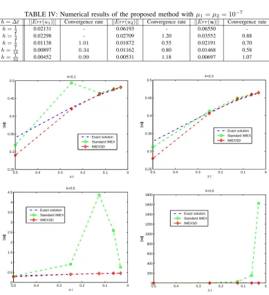
In Fig. 2, a plot of ||u|| computed by each of the solution methods and exact solution for decreasing time step size is given. In this figure, standard IMEX stands for the implicit-explicit time stepping without the SD method, IMEXSD represents the proposed method. From these plots,
µ1=µ2= 10−2, as the size of kgrows, it is observed that
the stability of the standard IMEX method decreases, but the IMEXSD method is more exact and effective.
In Fig. 3, the isovalues of u are compared to exaction isovalues by the standard IMEX and IMEXSD methods respectively. In these plots, we choose k = 0.5 and µ1 =
µ2= 10−2.
In summary, these experiments confirm the efficiency of our proposed method.
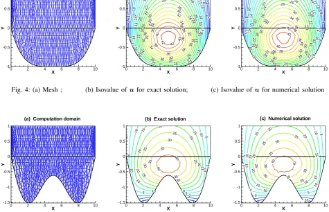
B. Example 2
We consider a coupled system withΩ1= (0,10)×(0,1)
andΩ2={(x, y) :
16(x−5)4
104 −1≤y≤0, x∈(0,10)}.Let
{
u1=x(10−x)(1−y)exp(−t),
u2=x(10−x)(c1+c2y+c3y2)exp(−t),
where c1, c2 and c3 are determined by the interface
condition. In this example, we choose k = 1,
µ1 = µ2 = 10−3, ∆t = 0.0002 and T = 0.2 (i.e.,
1000 time steps). The mesh and isovalue of u for exact solution and numerical solution are shown in Fig. 4.
C. Example 3
In this example we assume that there is a submarine mountain (i.e., the subdomainΩ2 is nonconvex) whereasΩ1
is the same as in Example 2.Ω2is given by
Ω2={(x, y) : 0≥y≥α−0.175(2x−10) sin(0.35(2x−10)),
x∈(0,10)},
where α = 1.75 sin(3.5). The boundary and initial conditions are the same as Example 2. In this example, we choosek= 1,µ1=µ2= 10−3,∆t= 0.0002andT = 0.2
(i.e., 1000 time steps). The mesh and isovalue of u for exact solution and numerical solution are shown in Fig. 5. We can notice that the presence of the submarine mountain dramatically affects the flow in Ω2. Indeed, the flow slows
down before arriving to the straitness and accelerates again after crossing it.
VI. CONCLUSION
We present a new implicit-explicit time stepping scheme based on the SD method for the two domain convection-dominated convection-diffusion-reaction problem. The pro-posed method provides a convenient decoupling strategy for
IAENG International Journal of Applied Mathematics, 48:3, IJAM_48_3_06
TABLE I: Numerical results of the standard implicit-explicit method withµ1=µ2= 10−1
h= ∆t ||Err(u1)|| Convergence rate ||Err(u2)|| Convergence rate ||Err(u)|| Convergence rate
h=12 0.01905 - 0.06499 - 0.06773
-h=1
4 0.02466 - 0.02644 1.30 0.03616 0.91
h=18 0.04221 - 0.02982 - 0.05168
-h= 161 0.00501 3.07 0.00605 2.30 0.00785 2.72
h= 1
32 0.00229 1.13 0.00267 1.18 0.00352 1.16
TABLE II: Numerical results of the proposed method withµ1=µ2= 10−1
h= ∆t ||Err(u1)|| Convergence rate ||Err(u2)|| Convergence rate ||Err(u)|| Convergence rate
h=1
2 0.01811 - 0.07986 - 0.08189
-h=14 0.03929 - 0.03510 1.19 0.05268 0.64
h=18 0.02865 0.46 0.02343 0.58 0.03701 0.51
h= 1
16 0.00444 2.70 0.00585 2.00 0.00734 2.33
h= 321 0.00228 0.96 0.00263 1.15 0.00348 1.08
TABLE III: Numerical results of the proposed method withµ1=µ2= 10−3
h= ∆t ||Err(u1)|| Convergence rate ||Err(u2)|| Convergence rate ||Err(u)|| Convergence rate
h=12 0.02127 - 0.06213 - 0.06567
-h=1
4 0.02300 - 0.02706 1.20 0.03551 0.89
h=18 0.01114 1.05 0.01843 0.55 0.02153 0.72
h= 161 0.00783 0.51 0.01059 0.80 0.01318 0.71
[image:8.595.104.494.326.753.2]h= 321 0.00395 0.99 0.00469 1.18 0.00613 1.10
TABLE IV: Numerical results of the proposed method withµ1=µ2= 10−7
h= ∆t ||Err(u1)|| Convergence rate ||Err(u2)|| Convergence rate ||Err(u)|| Convergence rate
h=12 0.02131 - 0.06193 - 0.06550
-h=14 0.02298 - 0.02709 1.20 0.03552 0.88
h=18 0.01138 1.01 0.01872 0.55 0.02191 0.70
h= 161 0.00897 0.34 0.01162 0.80 0.01468 0.58
h= 321 0.00452 0.99 0.00531 1.18 0.00697 1.07
0 0.1 0.2 0.3 0.4 0.5 0.25
0.3 0.35 0.4 0.45 0.5
∆ t
||
u
||
k=0.1
Exact solution Standard IMEX IMEXSD
0 0.1 0.2 0.3 0.4 0.5 0.25
0.3 0.35 0.4 0.45 0.5
∆ t
||
u
||
k=0.3
Exact solution Standard IMEX IMEXSD
0 0.1 0.2 0.3 0.4 0.5 0 0.5 1 1.5 2 2.5 3 3.5 4 4.5
∆ t
||
u
||
k=0.5
Exact solution Standard IMEX IMEXSD
0 0.1 0.2 0.3 0.4 0.5 0 200 400 600 800 1000 1200 1400 1600 1800
∆ t
||
u
||
k=0.6
Exact solution Standard IMEX IMEXSD
Fig. 2: Stability of uas ∆t→0, different values ofk
IAENG International Journal of Applied Mathematics, 48:3, IJAM_48_3_06
-0 .4 -0 .4 -0 .4 -0 .2 -0 .2 -0.2 0 0 0 0 0 0 0 0 .2 0.2 0.2 0.2 0.2 0 .4 0.4 0 .4 0 .6 0 .6 0 .6 0 .8 0 .8 0 .8 1 1 1 1 .2 1.2 1 .2 1 .41.4 1.4 X Y
0 0.2 0.4 0.6 0.8 1
-1 -0.5 0 0.5 1 (a) IMEX 0 .01 0 .0 1 0 .0 1 0 .0 1 0.0 1 0.0 2 0 .0 2 0 .02 0 .0 2 0 .02 0.0 3 0 .0 3 0 .0 3 0 .0 3 0.0 3 0 .0 4 0 .0 4 0 .0 4 0 .04 0.0 4 0.0 5 0 .0 5 0 .05 0 .0 5 .05 0.0 6 0.0 6 0 .0 6 0 .06 0 .06 0.0 6 0.07 0.0 7 0.07 0.07 0 .07 0 .0 7 0.0 8 0.08 0.08 0.08 0 .08 0 .08 0.0 9 0.09 0.09 0.09 0 .0 9 0 .09 0.1 0 .1 0.1 0.1 0.1 0.1 0.1 0.11 0 .11 0 .11 0.11 0.11 0.1 1 0.12 0 .12 0.12 0.12 0.1 2 0 .1 3 0.13 0.1 3 0.13 0.13 0.14 0 .14 0.14 0.1 4 0.15 0.1 5 0.15 0.15 0.16 0.1 6 0.16 0.16 0.1 7 0.1 7 0.17 0.1 8 0 .1 8 X Y
0 0.2 0.4 0.6 0.8 1
-1 -0.5 0 0.5 1
(b) Exact solution
0 .01 0 .0 1 0 .0 1 0 .0 1 0.0 1 0.0 2 0 .0 2 0 .0 2 0 .02 0.0 2 0.0 3 0 .0 3 0 .03 0 .0 3 0.0 3 0 .0 4 0 .0 4 0 .04 0 .0 4 0.0 4 0.0 5 0 .0 5 0 .05 0 .0 5 0.05 0.0 6 0.0 6 0 .0 6 0 .06 0 .0 6 0.0 6 0.07 0.0 7 0.07 0.07 0 .0 7 0 .07 0.0 8 0.08 0.08 0.08 0 .08 0.0 8 0.0 9 0.09 0.09 0.09 0 .0 9 0.09 0.1 0 .1 0.1 0.1 0 .1 0.1 0.1 0.11 0 .11 0.1 1 0.11 0.11 0.1 1 0.12 0 .1 2 0.12 0.12 0.1 2 0 .1 3 0.13 0.1 3 0.13 0.1 3 0.14 0 .1 4 0.14 0 .1 4 0.15 0.1 5 0.15 0.15 0.16 0.1 6 0.16 0.16 0.1 7 0 .17 0.17 0.18 0 .18 X Y
0 0.2 0.4 0.6 0.8 1
-1 -0.5 0 0.5 1 (c) IMEXSD
Fig. 3: (a) Isovalue ofu by standard IMEX ;(b) Isovalue ofuby exact solution; (c) Isovalue ofu by IMEXSD
X
Y
0 2 4 6 8 10
-1 -0.5 0 0.5 1
(a) Computational domains
2 2 4 4 6 6 6 8 8 8 1 0 10 12 12 1 2 14 1 4 1 4 14 1 6 16 1 6 16 16 16
18 18
18 18
20 20 20 20 20 20 2 0 22 22 22 2 2 22 22 2 2 24 24 24 24 24 2 4 26 26 26 2 6 26 26 28 28 2 8 28 2 8 30 30 3 0 30 30 32 32 3 2 32 32 34 34 34 34 36 36 36 36 38 3 8 40 40 40 42 42 X Y
0 2 4 6 8 10
-1 -0.5 0 0.5 1
(b) Exact solution
2 2 2 4 4 4 6 6 6 6 8 8 1 0 10 10 1 0 12 12 1 2 12 14 14 1
41 14
6 16 16 16 1 6 18 18 18 18 18 20 20 20 20 2 0 20 20 2 0 22 22 22 2 2 22 22 24 24 2 4 24 24 26 26 26 26 26 28 28 28 28 28 2 8 30 30 30 30 30 32 32 32 32 34 34 34 36 36 36 38 38 40 40 42 X Y
0 2 4 6 8 10
-1 -0.5 0 0.5 1
(c) Numerical solution
Fig. 4: (a) Mesh ; (b) Isovalue ofu for exact solution; (c) Isovalue ofufor numerical solution
X
Y
0 2 4 6 8 10
-1.5 -1 -0.5 0 0.5 1
(a) Computation domain
0 0 5 5 5 5 5
10 10
10
10 10
1
0
15 15
15 1 5 20 20 20
20 2
0 25 25 25 2 5 30 3 0 30 35 35 35 40 40 X Y
0 2 4 6 8 10
-1.5 -1 -0.5 0 0.5 1
(b) Exact solution
-10 0 0 0 5 5 5 5 5 1 0 10 1 0 10 10 15 1 5 1 5 15 15 20 20 20 20 20 25 25 2 5 25 30 30 3 0 35 3 5 35 40 40 X Y
0 2 4 6 8 10
-1.5 -1 -0.5 0 0.5 1
(c) Numerical solution
Fig. 5: (a) Mesh ; (b) Isovalue ofufor exact solution; (c) Isovalue ofufor numerical solution
large problems, allowing easy implementation of subdomain solvers. At each time step data is explicitly passed across the interface and the decoupled subdomain equations are then solved in parallel. In addition, stability and convergence are maintained. Further study is underway to improve the simulation by extending to more realistic problems.
ACKNOWLEDGMENT
The authors would like to thank the editor and anonymous reviewers for their valuable comments and helpful sugges-tions on the quality improvement of our present paper.
REFERENCES
[1] M. Asadzadeh, E. Kazemi and R. Mokhtari, Discrete-ordinates and streamline diffusion methods for a flow described by BGK model, SIAM J. Sci. Comput., vol. 36, pp. 729-748, 2014.
[2] S. C. Brenner and L. R. Scott, The Mathematical Theory of Finite Element Methods, Springer-Verlag, 2002.
[3] D. Bresch and J. Koko, Operator-splitting and Lagrange multiplier do-main decomposition methods for numerical simulation of two coupled Navier-Stokes fluids, Int. J. Appl. Math. Comput. Sci., vol. 16, pp. 419-429, 2006.
[4] E. Burman and M. A. Fern´andez, Stabilized explicit coupling for fluid-structure interaction using Nitsche’s method , C. R. Math. Acad. Sci. Paris, vol. 345, pp. 467-472, 2007.
[5] P. Causin, J . F. Gerbeau and F. Nobile, Added-mass effect in the design
IAENG International Journal of Applied Mathematics, 48:3, IJAM_48_3_06
[image:9.595.56.530.56.193.2] [image:9.595.55.531.271.577.2] [image:9.595.43.527.438.580.2]of partitioned algorithms for fluid-structure problems, Comput. Methods Appl. Mech. Engrg., vol. 194, pp. 4506-4527, 2005.
[6] L. Chen and J. Xu, Stability accuracy of adapted finite element methods for singularly perturbed problems, Numer. Math., vol. 109, pp. 167-191, 2008.
[7] J. M. Connors, J. S. Howell and W. J. Layton, Partitioned time stepping for a parabolic two domain problem, SIAM J. Numer. Anal., vol. 47, pp. 3526-3549, 2009.
[8] S. Franz, SDFEM with non-standard higher-order finite elements for a convection-diffusion problem with characteristic boundary layers, BIT Numer. Math., vol. 51, pp. 631-651, 2011.
[9] S. Franz, R. Kellogg and M. Stynes, Galerkin and streamline diffusion finite element methods on a Shishkin mesh for a convection-diffusion problem with corner singularities, Math. Comput., vol. 81, pp. 661-685, 2012.
[10] P. Hansbo and A. Szepessy, A velocity-pressure streamline diffusion finite element method for the incompressible Navier-Stokes equation, Comput. Methods Appl. Mech. Engrg., vol. 84, pp. 175-192, 1990. [11] J. G. Heywood and R. Rannacher, Finite-element approximation of
the nonstationary Navier-Stokes problem. Part IV: Error analysis for second-order time discretization, SIAM J. Numer. Anal., vol. 27, pp. 353-384, 1990.
[12] A. Hiltebrand and S. Mishra, Entropy stable shock capturing space-time discontinuous Galerkin schemes for systems of conservation laws, Numer. Math., vol. 126, pp. 103-151, 2014.
[13] C. Johnson and U. Navert, Ananalysis of some finite element methods for advection-diffusion problems, in: O. Axelsson, L.S. Frank, A. VanderSluis(Eds.), Analytical and Numerical Approaches to Asymptotic Problems in Analysis, North-Holl and Publ., Amsterdam, (1981). [14] C. Johnson, Finite element methods for convection-diffusion problems,
in: R.Glowinski, J. Lions(Eds.), Computing Methods in Engineering and Applied Sciences, North-Holl and Publ., Amsterdam, (1981). [15] C. Johnson, U. Navert and J. Pitkaranta, Finite element methods for
linear hyperbolic problems, Comput. Methods Appl. Mech. Engrg., vol. 45, pp. 285-312, 1985.
[16] C. Johnson and J. Saranen, Streamline diffusion methods for the incompressible Euler and Navier-Stokes equations, Math. Comp., vol. 47, pp. 1-18, 1986.
[17] C. Lehrenfeld and A. Reusken, Nitsche-XFEM with streamline diffu-sion stabilization for a two-phase mass transport problem, SIAM J. Sci. Comput., vol. 34, pp. 2740-2759, 2012.
[18] B. Liu, The analysis of a finite element method with streamline dif-fusion for the compressible Navier–Stokes equations, SIAM J. Numer. Anal., vol. 38, pp. 1-16, 2000.
[19] P. M¨uller , The Equations of Oceanic Motions, Cambridge University Press, Cambridge, UK, (2006).
[20] L. Z. Qian and H. P. Cai, Two-grid Method for Characteristics Finite Volume Element of Nonlinear Convection-dominated Diffusion Equations, Engineering Letters, vol. 24, pp. 399-405, 2016.
[21] T. J. Sun and K. Y. Ma, The finite difference streamline-diffusion methods for the incompressible Navier-Stokes equations, Appl. Math. Comput., vol. 149, pp. 493-505, 2004.
[22] T. J. Sun and D. P. Yang, The finite difference streamline-diffusion methods for Sobolev equation with convection-dominated term, Appl. Math. Comput., vol. 125, pp. 325-345, 2002.
[23] L. Tobiska and R. Verf¨urth, Analysis of a streamline diffusion finite element method for the Stokes and Navier-Stokes equations, SIAM J. Numer. Anal., vol. 33, pp. 107-127, 1996.
[24] G. D. Zhang, Y. He, and Y. Zhang, Streamline diffusion finite element method for stationary incompressible magnetohydrodynamics, Numer. Methods for Partial Differential Equations., vol. 30, pp. 1877-1901, 2014.
Ling-zhi Qianwas born in Lingbi, Anhui Province, china, in 1980. The author received his Ph. D. in computational mathematics at Nanjing Normal University, Nanjing, Jiangsu Province, China, in June 2016.
The author current research interests include numerical solution of partial differential equations and computing sciences, fluids and fluid-fluid interaction problems, two-phase fluids.