Determination of linear relations between systematic parts of variables with errors of observation the variances of which are unknown

The Economic and Social Review, Vol. 27, No. 2, January, 1996, pp. 87-117

Determination of L i n e a r Relations Between

Systematic Parts of Variables with E r r o r s

of Observation the Variances of Which

are Unknown*

R.C. G E A R Y

Department of Applied Economics, University of Cambridge

Abstract: Given a sufficient number of instrumental variables significantly correlated with the investigational variables, consistent estimates of the coefficients of the linear relations can be

determined (if they exist), without knowledge of the disturbance variances. The estimates are discussed from the viewpoint of probability convergence. In the case of two investigational and one instrumental variable, all three variables distributed on the normal surface, the distribution of the estimate of the coefficient is found exactly for all sample sizes, on certain hypotheses. The distribution function is remarkably simple. The applicability of the theorem to economic time series is discussed by (a) comparing the probability inferences derived from this Model A with those for the simplest stationary time-series model, termed Model B, and (b) by comparing the large-sample variances on several models. It is found that the theory can be used with confidence when the series are not too short and the error variances not too large. The theory is applied to a particular time series, showing that the accuracy of the estimate of the coefficient depends on the correlation between the instrumental variable and the two investigational variables. The theory to which reference is made in Sections II, III, and IV, relating to the two-investigational-variable case, is extended to many variables and tests are given, applicable when samples are not small, for determining the significance of coefficient estimates.

I I N T R O D U C T I O N

S

i n c e t h e a p p e a r a n c e i n 1934 o f R a g n a r F r i s c h ' s w e l l - k n o w n book Statistical Confluence Analysis by Means of Complete Regression Systems, s t a t i s t i c i a n s have come to recognize t h a t , w h a t e v e r else t h e y are, t h e classical regression equations are not f u n c t i o n a l r e l a t i o n s b e t w e e n t h e

v a r i a b l e s . Reiersol ( 1 9 4 1 , 1945) a n d Geary (1942, 1943) have s h o w n h o w relations, consistent i n t h e statistical sense, between variables can be derived. Reiers0l u s e d w h a t he t e r m e d t h e instrumental sets o f variables i n contra­ d i s t i n c t i o n t o t h e investigational set, w h i c h are the variables t h e systematic p a r t s o f w h i c h enter i n t o t h e relations; Reiersol's m e t h o d is t h a t used i n t h i s c o m m u n i c a t i o n . G e a r y showed h o w r e l a t i o n s c o u l d be established f r o m k n o w l e d g e o f t h e i n v e s t i g a t i o n a l set alone by h a v i n g recourse t o s e m i -i n v a r -i a n t s o f power greater t h a n t w o and of d-imens-ion greater t h a n u n -i t y .

I t i s assumed t h r o u g h o u t the paper t h a t t h e variances o f the disturbances are n o t k n o w n i n advance or cannot be efficiently estimated from t h e obser­ v a t i o n s . T h e d i s t u r b a n c e variances occur e x p l i c i t l y i n several f o r m u l a e , u s u a l l y i n order t h a t means a n d variances o f estimates a o f t h e coefficient o f r e l a t i o n s h i p , computed for different m a t h e m a t i c a l models, m a y be compared. I t w i l l be shown elsewhere (Geary, 1948) t h a t w h e n t h e disturbance variance is k n o w n or can be estimated a n d w h e n certain other conditions are satisfied, methods, o f e s t i m a t i o n o f t h e coefficients, more efficient i n t h e s t a t i s t i c a l sense t h a n those contemplated here, can be devised.

M o s t of t h e present paper is devoted to t h e frequency d i s t r i b u t i o n a n d t h e s a m p l i n g e r r o r s of t h e coefficient i n t h e simplest case, t h a t i n w h i c h a single r e l a t i o n is assumed to subsist between the systematic parts o f t w o variables. I n the final section, however, t h e errors i n t h e coefficients o f relations i n more t h a n t w o variables are dealt w i t h .

I I T H E P R O B L E M

M e a s u r e s of a r a n d o m sample of n of (2p - 1) variables i n t w o sets are observed:

where t h e xi t represent t h e measures of the i n v e s t i g a t i o n a l set a n d the xr t the measures of t h e i n s t r u m e n t a l set. Each variable of t h e l a t t e r set is s i g n i f i ­ c a n t l y correlated w i t h at least one variable o f the former set. I t w i l l be shown l a t e r t h a t t h e h i g h e r t h e correlation ( i n a sense defined) between the t w o sets t h e more efficient the estimates o f the coefficients of the l i n e a r r e l a t i o n .

E a c h o b s e r v a t i o n o f t h e i n v e s t i g a t i o n a l set is made subject t o error or

disturbance, i.e.,

(i) _xi t( i = l , 2 , - - , p ) '

(ii) (t = l , 2 , - , n ) ,

xi t =xi t + 4 > (1)

w h e r e x -t is t h e systematic p a r t a n d x"t t h e e r r o r or d i s t u r b a n c e . T h e f o l l o w i n g l i n e a r r e l a t i o n holds exactly (i.e., for a l l t ) between t h e systematic p a r t s :

i ai X;t= C , (2)

i=l

w h e r e C is a constant. I t is assumed t h a t t h e r e l a t i o n cannot be expressed i n fewer variables t h a n p. Estimates t h a t are consistent i n t h e s t a t i s t i c a l sense are derived for t h e coefficient ratios a j / a j . T h e m a i n object o f t h e paper i s to discuss t h e frequency d i s t r i b u t i o n o f these estimates w h i c h are f o u n d as follows. F r o m (2)

liai( x ;t- x ; ) = 0> (3)

w h e r e nx- = £t x -t. O n m u l t i p l y i n g by xr t a n d t a k i n g means o f n , we have

£ 0: ^ = 0 ( r = p + L p + 2 , - , 2 p - l ) , (4)

i=l

where

ni r = ^ i t ( x ;t- x ; ) xr t. (5)

A s s u m e t h a t t h e disturbances x ^ are i n d e p e n d e n t o f one a n o t h e r , o f t h e systematic p a r t s o f t h e i n v e s t i g a t i o n a l set, a n d of t h e i n s t r u m e n t a l set, t h a t t h e i r u n i v e r s a l means are zero, a n d t h a t the variances of t h e variables of t h e i n s t r u m e n t a l set are f i n i t e , w h i c h assumptions r u l e out, for t h e m o m e n t , a lagged i n v e s t i g a t i o n a l variable as a n i n s t r u m e n t a l v a r i a b l e . T h e systematic p a r t s x'it can be any n u m b e r s w h a t e v e r ; a n d i t is n o t necessary t o assume t h a t t h e e r r o r variance is t h e same for each t . I t follows t h a t t h e Reiers0l m e t h o d is applicable w h e n t h e variables are s t a t i o n a r y t i m e series, u n d e r u n r e s t r i c t i v e conditions. L e t

mi r = ^ I t ( Xi t - X; ) XH = 1 I t ( Xi t - Xj ) ( Xr t - Xr ) (6)

m rt>

so t h a t

E ( mi r- ni r) = 0 (8)

and

v a r ( mi r - ni r) = E ( mi r - ni r)2 = 0 ( l / n ) . (9)

I t follows t h a t ( mi r - n ^ ) tends i n p r o b a b i l i t y towards zero w i t h increasing n . We w r i t e

T h e r a t i o s a; / a1( i = 2,3,---,p), solutions of t h e simultaneous equations (10), are continuous functions of t h e mi r a n d hence t e n d i n probability towards the same functions o f the ni r — w h i c h , b y hypothesis, are d e t e r m i n a t e — i.e., the

T h e m e t h o d can, o f course, be used to estimate t h e coefficients o f more t h a n one l i n e a r r e l a t i o n b e t w e e n t h e systematic p a r t s o f the v a r i a b l e s , p r o v i d e d t h a t these r e l a t i o n s are i n t h e fewest v a r i a b l e s , w h i c h i m p l i e s , i n c i d e n t a l l y , t h a t no t w o r e l a t i o n s are such t h a t a l l t h e variables i n one appear i n t h e other. T h e m e t h o d i s accordingly n o t w e l l adapted t o t h e discovery o f structural r e l a t i o n s unless the f o r m o f these relations (i.e., t h e v a r i a b l e s t h a t t h e y contain) is g i v e n i n advance a n d satisfies t h e c o n d i t i o n j u s t specified.

T h e d i f f i c u l t y o f o b t a i n i n g a n u m b e r of i n s t r u m e n t a l variables h i g h l y correlated w i t h t h e i n v e s t i g a t i o n a l variables is, of course, a circumstance t h a t l i m i t s t h e usefulness o f t h e m e t h o d described i n t h i s section. W h e n t h e v a r i a b l e s are economic t i m e series Reiers0l has made t h e ingenious sugges­ t i o n t h a t lagged or f o r w a r d e d i n v e s t i g a t i o n a l variables can be used as i n s t r u ­ m e n t a l variables. T h i s m e t h o d usefully exploits t h e property characteristic of economic t i m e series, n a m e l y serial correlation. I n a p p l y i n g t h i s m e t h o d we w o u l d t a k e xi t( t = l , 2 , - - , n ) for one of t h e xr t. T h i s i n t r o d u c e s a s l i g h t c o m p l i c a t i o n i n t o t h e convergence i n p r o b a b i l i t y theorem, i n the proof t h a t ( ni r - mi r) converges i n p r o b a b i l i t y t o zero w h e n r = i . W e can easily show t h a t i n t h i s case E ( mi r - ni r) = 0 ( l / n ) a n d (as before) E ( mi r - ni r)2 = 0 ( l / n ) . I t is necessary t o assume i n a d d i t i o n t h e existence of t h e f o u r t h moments o f t h e errors.

I I I T H E E X A C T - F R E Q U E N C Y D I S T R I B U T I O N O F T H E C O E F F I C I E N T a

The problem dealt w i t h i n t h i s section is t h e simplest one t h a t can arise i n t h e order of ideas of t h i s paper, n a m e l y t h a t i n w h i c h t h e observed sample is

( xl t, x2 t, x3 t) ( t = L 2 , - - , n ) , of w h i c h xl t a n d x2 t are i n v e s t i g a t i o n a l a n d x3 t is i n s t r u m e n t a l . The following assumptions are made:

(i) (x

i t >x2 t >x3 t ) i s d i s t r i b u t e d o n t h e n o r m a l surface w i t h k n o w n variance-covariance m a t r i x ||fj.;j|| ( i , j = 1,2,3) t h e same for each t ; i n p r a c t i c e t h i s m a t r i x w i l l u s u a l l y have to be estimated from t h e sample;

(ii) the sets o f observations are s t a t i s t i c a l l y independent for different t ; (iii) the i n v e s t i g a t i o n a l variables xi t ( i = 1, 2) are t h e s u m o f a systematic p a r t x -t a n d a disturbance i n e r r o r x"t; as t h e l a t t e r are independent o f one another, o f the systematic parts, a n d of the i n s t r u m e n t a l variables, b o t h sys­ t e m a t i c parts a n d disturbances m u s t , by t h e C r a m e r - L e v y t h e o r e m , be each n o r m a l l y d i s t r i b u t e d .

I t is recognized t h a t t h i s theory is n o t f o r m a l l y applicable t o a n y plausible model o f economic t i m e series since, on account of t h e phenomenon of serial c o r r e l a t i o n , we cannot reasonably assume t h a t t h e frequency d i s t r i b u t i o n s are the same for different t : a t least t h e means should be deemed to alter. The application of the theorem to t i m e series is discussed i n d e t a i l i n t h e f o l l o w i n g section.

(iv) T h e r e l a t i o n x 'l t = ccx2 t + C holds e x a c t l y b e t w e e n t h e s y s t e m a t i c parts. The problem is to determine t h e frequency d i s t r i b u t i o n of t h e estimate a of the coefficient a given by

(11)

where

n

n X1= I ( xl t- x1) ( x3 t- x3) ,

(12)

t=i

n X2 - X t (x2 t ~x2 ^X3 t ~X3 ^ -L e t t h e j o i n t frequency o f ( xl t, x2 t, x3 t) be

(13)

where

3 3

w i t h

t h e l a t t e r b e i n g t h e e l e m e n t o f t h e r e c i p r o c a l m a t r i x II All ( o f w h i c h t h e d e t e r m i n a n t is A ) o f t h e variance-covariance m a t r i x llUyll T h e u n i v e r s a l means of xi t m a y be assumed to be zero, w i t h o u t loss of generality.

T h e characteristic function f ( s , t ) o f ( x1 ;x2) is

, n/2

f ( s>t } =f0 , 3 n /2 n .( 3n ) ' - £ expJKsXj + t X2) - \ I t I ; I j C C ^ X ^ }

w h i c h is k n o w n t o e q u a l1

where

I l d xl t d x2 t d x3 t

t

f . N(n-l)/2

U

«12 «13 _ is

n

A * = «21 a2 2 a2 3

_ i t n

« 3 i

-is » n

a3 2 _ i t

n a3 3 Hence

f (s, t ) = \1-—(k10s + k0 1t ) + - i - ( k2 0s2 - 2 kns t + k0 2t2)

-(n-l)/2

(16)

(17)

(18)

(19) n n

where, on u s i n g (15) a n d w e l l - k n o w n d e t e r m i n a n t a l properties, we have

k i o - P-13>

^01 = ^23'

^20 ~~ UllM-33 -M-13>

^11 = M-23^13 ~ M-12M-33 >

V —

*02 — M-22^33 _

^23-(20)

Geary (1944), generalizing a r e s u l t o f H . C r a m e r ( 1 9 3 7 ) ,2 has s h o w n t h a t the frequency d i s t r i b u t i o n o f a g i v e n by (11) can, u n d e r v e r y general conditions, be expressed i n the form

4>(a) = I I ds

2ki

9 f ( s , t )

. at _t=-as

w h i c h , applied t o (19), gives

<Ka) =

^ 3

H . d s l i k0 1 + ^ ( kn + kMa )

• U - ( k i o " k0 1a) + ^2 <k20 + 2 k n a + k0 2a 2)

-(n+l)/2

n

(21)

(22)

Suppose n is an odd number. I t is easy to show t h a t ( k2 0k0 2 - k n ) is always positive, hence t h a t

k20 + 2 k1 1a + k0 2a

is always positive. A c c o r d i n g l y set t h e l a s t expression i n t h e brackets { } i n (22) equal to

1 - - K ' i s ^ n

so t h a t

K + K ' = 2 ( k1 0- k0 1a ) ,

K K ' = - ( k2 0 + 2 kna + k0 2a2) ,

from w h i c h we infer t h a t

K - K ' = 2 { ( k1 0 - k0 1a )2 + ( k2 0 + 2 kna + k0 2a2 )}*

(23)

(24)

(25)

Hence K and K ' are r e a l quantities, positive and negative respectively.

I n t h e i n t e g r a l o n t h e r i g h t - h a n d side o f (22) r e g a r d s as a complex v a r i a b l e . The f u n c t i o n t o be i n t e g r a t e d has t h e n t w o poles each o f order ( n + l ) / 2 a t - n i / K a n d - n i / K ' , t h e former accordingly on t h e negative a n d t h e

l a t t e r o n the positive side o f the i m a g i n a r y axis. I f t h e f u n c t i o n be i n t e g r a t e d a r o u n d a closed contour consisting of t h e r e a l axis a n d t h e great semicircle below t h e r e a l axis, b y Cauchy's theorem the i n t e g r a l m u s t equal t h e residue at t h e pole - n i / K , w h i c h is found to be

( n - l ) ! ( n - l ) , ,(n-3)/2.t r „ , - „ , , . . , , , . • K K ( K - K ) { ( k2 0k0 1+ k „ k1 0) f n - 1

(26)

+ a ( knk0 1 + ki nkn 9) ) 10^02 >

T h i s m u s t be t h e f u n c t i o n (|>(a) r e q u i r e d since the i n t e g r a l a r o u n d t h e great circle is obviously zero. M a k i n g t h e s u b s t i t u t i o n

y = ( k0 1a - k0 1) / ( k2 0+ 2 kna + k0 2a ) 2vl

= ( H23a - H18 W W 3 3 - u2 3 " 2(M-l2M-33 " U23^13 >a + ^llM-33 " M-13 ^ (2 7>

1 ( H 2 3a- ^ 1 3 )2 - 1

a n d u s i n g (24), (25), a n d (27), we f i n d

())(a) da = n - 3

2 )

- ( l + y2) -n / 2d y , (28)

so t h a t y V n - 1 is d i s t r i b u t e d as t h e Gosset-Fisher t w i t h ( n - 1) degrees of freedom.

T h i s r e s u l t3 i s r e m i n i s c e n t o f t h a t o f Geary (1930) t h a t i f X\ a n d X2 are n o r m a l l y d i s t r i b u t e d w i t h X2 u n l i k e l y to assume negative values and

t h e n

a' = X i / X '2

y ' V n - 1 = (\i'01a -\i'lQ)/(|i;2a2 - 2 u 'na + \i'20V,

(29)

(30)

w h e r e j i '1 0 a n d \i'01 are t h e u n i v e r s a l means o f a n d X2 a n d \i'20 [i'n, a n d p.22 t h e variances and covariances, is n o r m a l l y d i s t r i b u t e d w i t h m e a n zero a n d variance u n i t y . W h a t w o u l d t h i s l a t t e r t h e o r e m show i f Xx a n d X2 given by (12) were n o r m a l l y d i s t r i b u t e d (as, of course, t h e y t e n d to be w h e n n tends t o w a r d s infinity)? We f i n d

y> f ^ 3 3 ^ 2 2a 2-2H i2a + ^ n | } 2 (31)

1 ( ^ 2 3a- ^ 1 3 )2 J

C o m p a r i n g (31) w i t h (27) (last expression) we see t h a t t h e y are i d e n t i c a l except for a change o f sign before t h e u n i t . A t first sight t h i s m i g h t appear to be a c o n t r a d i c t i o n since b o t h d i s t r i b u t i o n s m u s t i n t h e l i m i t , as n t e n d s t o w a r d s i n f i n i t y , be the same. The anomaly is explained by t h e fact t h a t t h e i d e n t i c a l first t e r m i n the brackets is of order n .

I n a p p l y i n g f o r m u l a (27) i t w i l l , of course, be necessary i n a l m o s t every case t o estimate the variance-covariance m a t r i x ||n.^|| from t h e observations. T h e corresponding Studentized problem o f f i n d i n g t h e d i s t r i b u t i o n of, e.g.,

2 " 2 2

m3 3( m2 2a - 2 m1 2a + mn) / m2 3( a - a ) (32)

where

a = m1 3 / m2 3 a n d cc = ( i1 3

/ R2 3> (33)

t h e m's being the sample values of the |a's, w o u l d appear to be o f considerable c o m p l e x i t y w h i c h m a y r e n d e r i t the more a t t r a c t i v e to s t a t i s t i c i a n s w i t h greater i n g e n u i t y t h a n the w r i t e r .

I n practical applications of the theorem one w i l l set i n the u s u a l w a y

f n3 3^2 2a2- 2 ^1 2a + un) V ^ x2 ( M )

1 ( ^ 2 3a- H i3)2 J n - 1

w h e r e x is t h e p r o b a b i l i t y p o i n t for t h e t - d i s t r i b u t i o n corresponding t o t h e p r e d e t e r m i n e d p r o b a b i l i t y 0.1, 0.05, 0.01, etc., so t h a t

H3 3 (^22& 2 ~ 2^ i 2a + t i n ) ^11 n ~ 1 = K (35)

( H 2 3 a - M 2 t2

0 > a2 ( K U2 3 ~ M-22M-33)- 2a(KM.1 3Ji23 - H 1 2 ^ 3 3 )+ ( K^ 1 3 ~ ^11^33)- (3 6)

A s a m e a s u r e o f t h e possible r a n g e o f v a r i a t i o n o f t h e estimate a correspond­ i n g t o a g i v e n p r o b a b i l i t y l e v e l we m a y t a k e t h e difference 8 of t h e roots of t h e expression o n t h e r i g h t o f (36). W e f i n d

2 { ^3 3K (H2 2H2 3 - 2H1 2^1 3^2 3 + ^N^ 23) - ^ 3 ( ^ 1 1 ^ 2 2 - ^ 1 2 ) }2

8 = - t • (37)

( K H 2 3 - M 3 3 )

B e a r i n g i n m i n d t h a t K i s a t t h e order o f n , a large-sample a p p r o x i m a t i o n to 5 is

2 r i ~

A = - ^ — ^ 3 3 ( ^ 2 2 ^ 1 3 - 2 a1 2a1 3^2 3 + ^uu23 ) 2. (38)

1 ^ 2 3 1 J

Perhaps t h e m o s t suggestive t r a n s f o r m a t i o n is t h a t found by s u b s t i t u t i n g

for Uy, w h e r e t h e | i ' a n d \i" r e p r e s e n t t h e variance-covariances o f t h e systematic a n d e r r o r p a r t s respectively of t h e observations. We f i n d

A = 2

l

i j

8

( n I

1

+ a V a ) ^ V

2

3 - (39)

T h e p r e c i s i o n o f t h e e s t i m a t e i n t h e large-sample case accordingly depends i n v e r s e l y o n a n d d i r e c t l y on U23 ( w h e n t h e variables xl t a n d x2 t are given) w h i c h is t a n t a m o u n t t o s t a t i n g t h a t we should select ( i f we have a choice) t h e i n s t r u m e n t a l v a r i a b l e w i t h t h e h i g h e s t c o r r e l a t i o n w i t h xl t a n d x^,- T h i s , o f course, i s j u s t w h a t w o u l d have been anticipated.

*3t = ICiX3 t - (40)

i=l

R e q u i r e d to f i n d t h e coefficients Cj so t h a t t h e v a r i a n c e is u n i t y a n d t h e covariance 1J.23 m a x i m u m , i.e.,

where

I V y C i C - 1 ,

i.j

j i .2 3 = X CjX; m a x i m u m

i

v ^ E x ^ / ^ E x ^

(41)

(42)

(43)

I n t h e u s u a l w a y t h e solution is given by

I j V y C - p ^ , (44)

where P is a Lagrange m u l t i p l i e r . Hence

c ^ P X j V1^ , (45)

w h i c h s u b s t i t u t e d i n (41) gives p: so t h e C; are k n o w n .

Consider t h e v e r y simple case i n w h i c h a l l t h e vy( i * j ) are equal to v a n d a l l t h e X.; to X, b o t h v a n d X b e i n g p o s i t i v e . Suppose, f u r t h e r , t h a t t h e v a r i a n c e s o f xa a n d x ^ are a l l u n i t y , so t h a t X a n d v are c o r r e l a t i o n coefficients. T h e n f r o m (39) i t w i l l be seen t o be advantageous i n t h e large-sample case t o t a k e for i n s t r u m e n t a l v a r i a b l e a w e i g h t e d m e a n o f t h e i n d i v i d u a l variables x ^ ' provided t h a t

( l i l j V g C i C j J V l i C i X j

l

2

*

1 (46)

= ( Z i C ? + 2 v I I cicj)2/ ^ Iici< - .

i < j X

Obviously t h e c; s h o u l d be a l l t a k e n as equal t o give t h e m i n i m u m value, so t h a t t h e i n e q u a l i t y w o u l d become

k + v k ( k - l )

w h i c h is always t r u e provided k > 1 since v < 1. A s a n example suppose k = 5 a n d v = 0.7. T h e n t h e i m p r o v e m e n t effected b y t a k i n g as i n s t r u m e n t a l v a r i a b l e a n average o f the five series, as compared w i t h u s i n g a n y one o f t h e m , w i l l be

(5 + 0 . 7 x 2 0 ) ^ / 5 = 0.87,

w h i c h is e q u i v a l e n t t o a n i m p r o v e m e n t i n accuracy o f 13 per cent as compared w i t h u s i n g any one of t h e m . E v e n i f we h a d available an i n f i n i t y o f i n v e s t i g a t i o n a l sets t h e i m p r o v e m e n t w o u l d be only 1 to v2, i.e., w h e n v = 0.7 by 16 per cent. N o m a t t e r w h a t approach is made to t h i s problem i m p r o v e d accuracy is difficult o f a t t a i n m e n t .

I V A P P L I C A T I O N T O E C O N O M I C T I M E S E R I E S

T h e t h e o r y o f r e l a t i o n s h i p b e t w e e n statistics finds i t s most i m p o r t a n t application i n economic t i m e series a n d i t is accordingly necessary to consider t h e s u i t a b i l i t y o f t h e s a m p l i n g m o d e l of Section I I I for d e a l i n g w i t h these k i n d s o f statistics. F o r m a l l y the model is i n a p p r o p r i a t e . W h i l e we m i g h t t a k e as t h e t h r e e - d i m e n s i o n a l n o r m a l4 u n i v e r s e t h e t h r e e series i n d e f i n i t e l y extended i n t i m e , i.e., as consisting of observations xi t ( i = 1, 2, 3; t = - N , - N + 1, N - 1, N , w h e r e N is i n d e f i n i t e l y large), for t h e theorem to apply t h e sample of n w o u l d have to be X jt j ( j = l , 2 , - - , n ) , where t h e t j are positive or negative integers selected at r a n d o m . I n practice t h i s w i l l h a r d l y ever be t h e case since t h e sample w i l l n e a r l y always consist of a series o f observations consecutive i n t i m e . W h a t is w a n t e d is a s a m p l i n g t h e o r y a p p r o p r i a t e t o

sequences of n , so t h a t w h e n we state t h a t t h e p r o b a b i l i t y is, say, 1/20 t h a t a

differs from a given a (Usually zero) b y a t least t h e a m o u n t found i n t h e g i v e n samples we m e a n t h a t w e should expect to f i n d approximately a p r o p o r t i o n o f 1/20 o f such cases i f t h e experiment were repeated a large n u m b e r of t i m e s for sequences o f n a t d i f f e r e n t n o n o v e r l a p p i n g p a r t s o f t h e i n d e f i n i t e l y extended t i m e series.

I t w i l l be s h o w n , however, t h a t for t i m e series o f moderate l e n g t h t h e t h e o r e m i n Section I I I can be a p p l i e d w i t h confidence and, as the p r a c t i c a l application considered i n Section V w i l l make a b u n d a n t l y clear, the theorem, w h i l e applicable t o samples of a l l sizes, w i l l , i n practice, y i e l d useful results only w h e n t h e samples are fairly large. I t w i l l be noted, i n t h e first place, t h a t a, g i v e n by (11), is s y m m e t r i c a l i n t h e t , so t h a t t h e order i n w h i c h t h e sets o f t h r e e ( xl t, x2 t, x3 t) are t a k e n is i m m a t e r i a l —- t h e sample sequence need not be envisaged as s e r i a l l y correlated. W e are accordingly quite at l i b e r t y

to r e g a r d t h e p a r t i c u l a r sample as a r a n d o m s a m p l e f r o m some t h r e e -d i m e n s i o n a l t i m e universe, i.e., sequences i n -d e f i n i t e l y exten-de-d i n t i m e . T h e

has t o be e s t i m a t e d f r o m t r o u b l e is t h a t t h e variance-covariance m a t r i x

t h e p a r t i c u l a r sample a n d we k n o w t h a t unless t h e sample series are v e r y l o n g (for example c o v e r i n g several periods i f t h e series are p e r i o d i c ) t h e estimates o f t h e m a t r i x cannot be regarded as s t a t i s t i c a l l y consistent: t h e estimates o f t h e variances i n p a r t i c u l a r w o u l d u s u a l l y be too l o w , i f , for instance, t h e sample series covered o n l y p a r t o f a p e r i o d . I n o t h e r w o r d s , different short sample sequences w o u l d y i e l d estimates of t h e variance t h a t for t h e g i v e n sample n u m b e r w o u l d v a r y more w i d e l y t h a n t h e y s h o u l d i f computed from completely r a n d o m samples a l l from t h e same universe.

N o w i t w i l l have been seen, from (27), t h a t t h e frequency d i s t r i b u t i o n o f a depends on t h a t of

_=l i3 3( ^2a2- 2 u1 2a + un) (4g)

( H23a- ^ i 3 )2 Set

M-12 - V ^ nu2 2 Pl2»

^13 - V ^ l # 3 3 Pl3>

^23 ~~ V^22^33 P23'

where the pjj are coefficients o f correlation. T h e n

z = ( a2 - 2 f 1 2p1 2a + x2 2) / ( p2 3a - P1 3T1 2)2 , (49)

w h e r e T1 2 = M-11/1*22 • T h e p o p u l a t i o n parameters are accordingly reduced t o four, c o n s i s t i n g o f x& a n d t h e t h r e e c o r r e l a t i o n coefficients. W h i l e t h e estimates o f u u a n d u2 2 f r o m t h e sample sequence w i l l be biased i t is plausible t o assume t h a t t h e estimate o f t h e i r r a t i o i 2 2 m i g h t be unbiased, p a r t i c u l a r l y h a v i n g r e g a r d t o the fact t h a t t h e system to be w o r k a b l e m u s t be a h i g h l y correlated one. N o r does t h e r e appear to be any good reason w h y t h e t h r e e correlation-coefficient estimates should be biased. I f i t does no more, t h i s aspect suggests t h a t t h e t h e o r e m of Section I I I m i g h t be adapted to t i m e series even i f these are serially correlated.

Comparison of Simplest Time-Series Frequency with Frequency of Section I I I

d i s t r i b u t i o n o f t h e e s t i m a t e f r o m a time-series model, o f t h e s i m p l e s t s t a t i o n a r y type. T h i s w i l l be t e r m e d Model B ( i n contra-distinction t o Model A of Section I I I ) a n d i s as follows:

T h r e e series of observations xi t( i = 1,2,3; t = l , 2 , - - , n ) are made a t equal t i m e i n t e r v a l s o f w h i c h t h e investigational sets xl t a n d x ^ are given by

xi t ~ xn + xi t >

X2 t - X2 t + X2 t >

(50)

w h e r e t h e systematic parts x 'l t and x2 t are connected by the exact r e l a t i o n

xl t- c e x2 t,

the same for a l l t . W e also assume t h a t

X txl t = 0 = X tx2 f

T h e a c t u a l sample i n v e s t i g a t i o n a l series are t h e n assumed t o consist i n systematic p a r t s x ^ a n d x2 t fixed once for a l l n o t only i n m a g n i t u d e b u t i n order, d i s t u r b e d b y x "t a n d x2 t assumed t o be n o r m a l l y d i s t r i b u t e d w i t h means zero a n d variances \i."n a n d u2 2, independent of one a n o t h e r of t h e s y s t e m a t i c p a r t s , a n d w i t h i n s t r u m e n t a l series x3 t ( w i t h Xtx3 t =0 ) al so r e g a r d e d as f i x e d f r o m sample to sample: t h i s i m p l i e s , of course, t h a t t h e

series x3 t is n o t a lagged i n v e s t i g a t i o n a l variable, a case considered later. The estimate a o f a on M o d e l B is t h e n

a = ^ l , (51)

where

X1 = X txi tx3 t »

X2 = X tx2 tX3 f

Clearly

E XX = X txi tx3 t = a£ tx2 tx3 t >

(52) E X2 = Z tx2 tx3 t '

2 _ " v 2

° x2 - ^ 2 2 - ^ tx3 t >

(53)

a n d Xx a n d X2 are stochastically independent. N o w a is t h e q u o t i e n t o f t w o n o r m a l variates Xx a n d X2 of w h i c h i t m a y be assumed t h a t t h e d e n o m i n a t o r X2 is u n l i k e l y to assume negative values. Hence by Geary (1930)

i s n o r m a l l y d i s t r i b u t e d w i t h m e a n zero a n d v a r i a n c e u n i t y for a l l s a m p l e sizes. T h i s s a m p l i n g model is so m u c h more simple t h a n M o d e l A t h a t i t is n a t u r a l t o i n q u i r e t h e reason w h y i t s h o u l d n o t be u s e d i n preference t o M o d e l A i n connection w i t h t h e t h e o r y o f l i n e a r r e l a t i o n s h i p i n t i m e or otherwise. T h e answer i s , of course, t h a t t h e essential feature o f t h e t h e o r y developed i n t h i s c o m m u n i c a t i o n is t h a t t h e e r r o r variances ux l a n d n2 2 are n o t k n o w n or cannot be efficiently estimated from t h e observations. W e can, however, assume t h e e r r o r variances k n o w n for t h e purpose of assessing t h e r e l i a b i l i t y o f M o d e l A as a p p l i e d t o t i m e series. I n o r d e r t o a p p l y M o d e l A f o r m a l l y t h e values of t h e variances a n d covariances r e q u i r e d are g i v e n by:

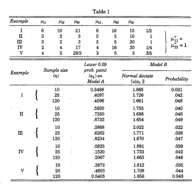
W e proceed as follows: G i v e n sample size n , t h e variances a n d covariances, a n d a g i v e n p r o b a b i l i t y (say 0.05), we f i n d t h e confidence l i m i t s ax a n d a2 o f t h e estimate a u s i n g t h e Model A theorem, i.e., d e r i v e d f r o m (36). T h e values ax (or a2) are s u b s t i t u t e d for a i n (54) a n d t h e ( n o r m a l ) p r o b a b i l i t y o f t h i s u n i t - v a r i a n c e d e v i a t i o n r e a d off for c o m p a r i s o n w i t h t h e g i v e n p r o b a b i l i t y (say 0.05). The results for five examples, w i t h t h r e e sample sizes ( n = 10, 25, 120) for each, are given i n Table 1. The variances, covariances, a n d coefficient a for each example are shown at t h e head of t h e t a b l e . T h e examples are designed to i l l u s t r a t e t h e different k i n d o f cases t h a t can occur, i n p a r t i c u l a r (i) different m a g n i t u d e s o f e r r o r variances, ( i i ) different correlations b e t w e e n i n s t r u m e n t a l v a r i a b l e a n d i n v e s t i g a t i o n a l variables, ( i i i ) different values o f a ( w h i c h w i t h o u t loss o f g e n e r a l i t y m a y be assumed n o t t o exceed u n i t y ) . A c t u a l l y t h e u n i t s i n w h i c h t h e i n v e s t i g a t i o n a l v a r i a b l e s are m e a s u r e d are deemed to be such t h a t t h e error variances, i.e., and u2 2, are each u n i t y .

u

a E X2- E X

(54)

W i i = + I t x' i t > n u 13 = I t xi tx3 t nM-12 ~ 2 , txl tX2 t > nM-23 ~~ ^ tX2 tX3 t

& /2 2

n j l22 = nM-22 + I tx2 t > n U3 3 = I tx3 f

[image:16.472.35.417.52.425.2]

Table 1

Example _{Mil Hl2 A<22 Ml3. As}

I 6 10 21 8 16 15 1/2 ,

n m rv 3 2 3 2 2 4 3 5 3 5 17 4 5 5 16 10 20 20 1 1

1/4 i4> = i

V 4 5 28/3 3 5 3 3/5 J

Lower 0.05 Model B

Sample size (n)

prob. point

Model A

Example Sample size

(n)

prob. point

Model A

Normal deviate „ , ....

[ u ( a i a Proia&ifc*

10 0.3488 1.865 0.031

\

|

25 .4097 1.726 .042

1 120 .4596 1.661 .048

10 .5920 1.755 .040

II { 25 .7350 1.688 .046

120 .8732 1.654 .049

f 10 .3868 2.022 .022

m

j

25 .6262 1.771 .038

120 .8234 1.670 .047

10 .0823 1.891 .029

rv | 25 .1520 1.733 .042

120 .2067 1.663 .048

10 .3872 1.812 .035

v

J

25 .4693 1.708 .044

120 0.5405 1.658 0.049

Since, as s h o w n l a t e r on, t h e variances on M o d e l A and M o d e l B t e n d to t h e same v a l u e w h e n n t e n d s t o w a r d s i n f i n i t y , i t is t o be expected t h a t t h e t w o models w o u l d y i e l d f a i r l y s i m i l a r results (i.e., w o u l d give m u c h t h e same l i m i t s for t h e range o f values of t h e estimate a o f a corresponding t o a given p r o b a b i l i t y ) for samples o f moderate size. Table 1 shows t h a t t h i s is a c t u a l l y t h e case. E v e n for samples as s m a l l as 25 t h e p r o b a b i l i t y of t h e lower l i m i t ax ( s h o w n i n t h e f i n a l c o l u m n ) is riot very different from the p r o b a b i l i t y 0.05. Since i n a l l cases t h e M o d e l B p r o b a b i l i t y is "below t h a t of M o d e l A (0.05) i t is clear t h a t t h e l i m i t s d e r i v e d from t h e l a t t e r are on the "safe side". T h i s also is t o be expected since i n a p p l y i n g M o d e l B we assume more i n f o r m a t i o n t h a n i n a p p l y i n g t h e other m o d e l , n a m e l y t h a t t h e error variances are k n o w n . I n t h e table iattention has been confined to the lower l i m i t ax: t h e upper l i m i t a2 w o u l d n o t give s i g n i f i c a n t l y different probabilities i n the last column.

h i g h l y c o r r e l a t e d w i t h t h e i n v e s t i g a t i o n a l v a r i a b l e s y i e l d m o r e accurate estimates o f t h e coefficient (as shown i n t h e paper) b u t i t r e s u l t s i n more s i m i l a r inferences f r o m Models A a n d B . T h i s is c l e a r l y seen b y c o m p a r i n g examples I I and I I I w h i c h are i d e n t i c a l except for 1133 w h i c h is t w i c e as large i n I I I as i n I I . R e l a t i v e l y large e r r o r variances (as i n d i c a t e d b y r e l a t i v e l y s m a l l values o f |0.u a n d H22) d ° not appear t o render t h e r e s u l t s m o r e d i s ­

cordant, i.e., i n g i v i n g M o d e l A probabilities very different from 0.05; t h i s w i l l be seen from example I I i n w h i c h the e r r o r variances are r e l a t i v e l y large a n d y e t t h e probabilities are nearest to 0.05 for a l l sample sizes.

I t is emphasized t h a t t h e t w o frequency d i s t r i b u t i o n s u t i l i z e d i n Models A a n d B are exact, assuming o f course, t h a t t h e conditions o f t h e theorems are satisfied. The examples s t r o n g l y suggest t h a t t h e M o d e l A approach yields s a m p l i n g l i m i t s for estimates o f a (corresponding t o a g i v e n p r o b a b i l i t y ) w h i c h do n o t differ w i d e l y f r o m those o f t h e " t i m e series" M o d e l B , for samples of moderate size.

I t is i n t e r e s t i n g t o compare the q u a d r a t i c i n e q u a l i t i e s y i e l d i n g t h e l i m i t s f r o m t h e t w o models. The M o d e l A e q u a t i o n , w h i c h is d e r i v e d f r o m (36) by s u b s t i t u t i n g ( \ i 'n + un) a n d ( \ i '2 2 + M-^) * °r ^22 respectively, m a y be

r e w r i t t e n as

follows:-( K U2 3 - u2 2u3 3) ( a - a )2 - M.33(a2M.22 £ °> <5 6)

whereas the M o d e l B quadratic i n e q u a l i t y , derived from (54) is

K V 23( a - a )2- H33( a2U 2 2 + l ^ i i )s 0- <5 4' )

I n ( 5 6 )5 K = 1 + nJx2 where x is the p r o b a b i l i t y p o i n t from t h e t - d i s t r i b u t i o n

corresponding t o a g i v e n p r o b a b i l i t y a n d K ' = vJi% w h e r e i, is t h e n o r m a l

p r o b a b i l i t y p o i n t corresponding to t h e same p r o b a b i l i t y . Since K a n d K ' t e n d t o w a r d s t h e same l i m i t of order n w h e n n tends t o w a r d s i n f i n i t y i t is clear t h a t t h e l i m i t s derived from the t w o equations m u s t t e n d to be t h e same.

Comparison of Variances of Consistent Estimates of the Coefficient a

I n t h e four f o l l o w i n g subsections large-sample a p p r o x i m a t i o n s are placed on record of means a n d variances o f estimates o f t h e coefficient a u s i n g four different models or methods, i n c l u d i n g Models A a n d B already discussed. The general objective is to show t h a t where t h e samples are moderately large, a n d t h e error or disturbance variances r e l a t i v e l y s m a l l , t h e approximations to

means a n d variances o f a on t h e different assumptions do not differ m u c h . Somewhat h e u r i s t i c a l l y t h e inference is made t h a t the frequency d i s t r i b u t i o n appropriate to one is approximately applicable to a l l ; i n simple t e r m s t h a t t h e t h e o r y o f Section I I I m a y be used w i t h confidence i n t i m e series, unless t h e sequence is short. T h e approximations t o t h e means a n d variances w h e n t h e i n s t r u m e n t a l v a r i a b l e is a lagged observational v a r i a b l e w i l l probably be found useful.

To t r a n s l a t e t h e variance-covariance m a t r i x | h ; j | i n t o time-series t e r m s we take

^ = E i it(X;t+x; ; ) ( x ; .t+ x p

= 8y K i +^ I txi txj t ( i , j = 1,2,3),

where observational variables are xl t a n d and t h e i n s t r u m e n t a l v a r i a b l e is

X& — t h e l a t t e r m a y be a lagged observational v a r i a b l e — t h e are t h e

e r r o r or d i s t u r b a n c e variances, a n d t h e systematic p a r t s of t h e v a r i a b l e s

X jt( j = 1,2,3) are regarded as fixed once for a l l .

Case when Instrumental Variable is a Lagged (or Advanced) Investigational Variable: Model C

I t w i l l p r e s e n t l y be shown t h a t , w h i l e t h e s a m p l i n g theory i n t h i s case is m u c h m o r e c o m p l i c a t e d t h a n w h e n t h e i n s t r u m e n t a l v a r i a b l e i s n o t a n i n v e s t i g a t i o n a l v a r i a b l e , t h e e r r o r w i l l be s l i g h t i f t h e s i m p l e t h e o r y a p p r o p r i a t e t o t h e l a t t e r case be assumed to apply f o r m a l l y t o t h e f o r m e r case, for samples o f moderate size. W e w i l l , i n fact, proceed t o compute t h e approximate m e a n a n d variances of t h e estimate a of a for the t w o cases. L e t

1 n

— Z ( X 'l t + X i 't) ( X2 t_1 + X ^ V i )

b = U f 1 (57)

— Z ( X2 t+ X2 t) ( X2.t_1 + X2 t_1)

n t=l

and

X 'l t = p X2 t (58)

exactly, w h e r e t h e systematic p a r t s X jt( i = L,2) are fixed once for a l l and stochastic v a r i a t i o n is i n t r o d u c e d only t h r o u g h the errors or disturbances X-^, assumed n o r m a l l y d i s t r i b u t e d w i t h means zero a n d variance f i n i t e , t h e same for a l l t .

I t ^ ' i t - 0 - ZtX2t,

i.e., t h a t w h i l e t h e systematic parts, deemed fixed from sample t o sample, are u n k n o w n , t h e i r sums are zero, effected i n practice by m e a s u r i n g t h e obser­ v a t i o n s from t h e i r means. B y t h e transformations

xi t= xi t/ cx ;t>

x

; ; = x ; ; / c

x ; ;

, a = 1,2) (59)

we f i n d

w i t h

1 ~ r / ft w / ft \

~ ^ t V Xl t + Xl tJ U 2 . t - l + x2 - t - l ' ' c

a = ^ = ^ b , (60)

— Z t (x2 t + X2 t ^X2 t - l + X2 t - l ) °xi't n

Xl t= ( X X2 t > (6 1)

a n d n o w w i t h t h e e r r o r variances ( o f X jt a n d x2 t) e q u a l t o u n i t y . T h e n u m b e r s x 'l t ( a n d x2 t f r o m (61)) are fixed f r o m sample to sample a n d can assume a n y f i n i t e v a l u e s w h a t e v e r . F r o m (60) i t w i l l be seen t h a t t h e coefficient o f v a r i a t i o n (the r a t i o o f t h e m e a n to t h e s t a n d a r d d e v i a t i o n ) o f a w i l l be equal to t h a t o f b for different samples o f n . To estimate large-sample approximations o f m e a n a n d variance o f a, set

2 tx2 tx2 t - i = V n u , ItX itX 2t_ i = V n x ,

I tx2 t - ixi ' t = V n v , X t x M t - i = ^ y ' (62) I tx2 t - ix2 t = V n w ,

whence

n E u2 = Itx2 2 t = n u2 2 = n ( | j .2 2 - 1 ) ,

n E v2 = n E w2 = Itx22 _x = n u3 3 = n ( u3 3 - 1 ) ,

(DO;

E x2= E y2 = l ,

-F r o m (60) a n d (61)

u2 3V n ( a - a ) = {v + x - a ( w + y ) H l + — ^ = ( u + w + y ) l , (64)

{ ^ 2 3 ^n J

where

nM-23 = £ tx2 tX2 t - l - (65)

Whence [ n o t i n g t h a t a3 3 = \i22 + 0 ( 1 / n ) ]

n ( i2 3E ( a - a ) - u2 2 + v ) a

n ^2 3E ( a - a )2 - ^3 3( l + a2) + - ^ { 2 ( 3 u22 - 4 ^2 3) ( l + 2 a2) - 3 ^2 2( l + a2) } (66)

n u2 3 1 J

+- ^ - { ^ 2 2 ( l + 3 a2) + v a2} .

n a2 3 1 J

These f o r m u l a e give E(a - a ) correct t o 0 ( n- 1) a n d E(a - a )2 to 0 ( n- 2) . Hence v a r (a) is d e r i v a b l e t o 0 ( n ~2) . U s i n g (59) t h e r e w i l l be no d i f f i c u l t y about finding means (b) a n d v a r (b) i n t e r m s of t h e covariances a n d variances of t h e o r i g i n a l variables Xi t = X -t + X - t ( i = 1,2) a n d of t h e error variances v a r (X-^).

Instrumental Variable not a Displaced Investigational Variable: Model D

I n t h i s case i n (57) we have X3t a n d X3t i n s t e a d o f X2 t_ j a n d X2t_1 respectively, w h e r e t h e observed i n s t r u m e n t a l v a r i a b l e X3t = X3t + X3 t. The disturbances X'lt, X2 t, X3t are c o m p l e t e l y i n d e p e n d e n t o f one another. B y analogous t r a n s f o r m a t i o n s we find i n s t e a d of (60)

^ Z t (xi t+ Xl t XX3 t+ X3 t ) 0 „

a = 4± = - ^ b , (67) - Zt ( x2 t + x2 t ) ( x3 t + x3 t)

w i t h x 'l t = ocx2 t a n d w h e r e , as before, t h e error variances, i.e., o f x ' ^ , x2 t, a n d x3 t, are n o w u n i t y a n d t h e i r means zero. W e r e a d i l y f i n d

n | i2 3E ( a - a ) - ( i3 3a , (68)

n u |3E ( a - a )2 ^ ( l+a2 ) L 3 _ 1 + 3 ^ 2 2 3 ^ 3 ( l + 3 « 2 ) ( f i 9 )

Displacement Effects

Suppose t h a t we s u b s t i t u t e f o r m a l l y i n (68) a n d (69) t h e variances a n d covariances t h a t w o u l d be found i f

x

2t

-i

were used as i n s t r u m e n t a l v a r i a b l e

i n s t e a d o f x ^ . Denote by X1 a n d X2 t h e r e s u l t i n g pseudo-values o f E(a - a)

a n d E ( a - a ) 2 . T h e n

n ^ X i - u ^ a , (70)

n u2 3X2M l + a2)

H3 3 n

4 ^ + { 2 u2 2 ( 1 + 2 a2) - u2 2 ( 1 + a2) } . (71)

T h e n from (65), (66), (70), a n d (71),

n a23 { E ( a - a ) - X1} - v a , (72)

n2u2 3 { E ( a - a )2 - X2 } - 2( 1 + 3 a2 ) ( 3 v u2 2 - 2 a2 3) + 6 v2a2. (73)

F o r m u l a e (72) a n d (73) i n d i c a t e t h e a p p r o x i m a t e effect o f u s i n g a lagged i n v e s t i g a t i o n a l v a r i a b l e as a n i n s t r u m e n t a l v a r i a b l e : t h e expressions on t h e r i g h t m a y be regarded as t h e "displacement effects". To form a more precise idea of t h e i r magnitude, set

M-23 = PlM-22'

V = P2U22>

where p i and p2 are serial correlations lagged 1 a n d 2 respectively. T h e n

n p2u2 2 { E ( a - a ) - X j - p2a , (72')

n2p ^2 2{E<a - « )2 - x2 } "2(1+ 3«2 K 3 p2 " 2P i ) + 6P 2a 2• (7 3' )

U s u a l l y px is about 0.9 and p2 about 0.7. S u b s t i t u t i n g these values t e n t a t i v e l y

we find

n u2 2 {E(a - a ) - X1} ~ 0.9a,

n2| i2 2| E ( a - a )2- X2} ~ L 5 + 8.9 a2

(72")

(73")

e r r o r s t a n d a r d d e v i a t i o n : i n fact t h e s m a l l e r t h e e r r o r t h e l a r g e r w i l l be H-22- I t

i s c l e a r t h a t for s a m p l e s o f m o d e r a t e s i z e n o g r e a t d i s t o r t i o n i s i n t r o d u c e d

i n t o t h e p r o b a b i l i s t i c i n f e r e n c e s b y u s i n g a d i s p l a c e d i n v e s t i g a t i o n a l v a r i a b l e

a s t h e i n s t r u m e n t a l v a r i a b l e a n d t r e a t i n g i t e x a c t l y a s i f i t s e r r o r c o n s t i t u e n t

w e r e i n d e p e n d e n t of t h o s e of t h e i n v e s t i g a t i o n a l v a r i a b l e s .

Model B Approximation

I t w i l l be n e c e s s a r y a l s o to c o n s i d e r t h e l a r g e - s a m p l e a p p r o x i m a t i o n s to t h e

m e a n a n d v a r i a b l e s for M o d e l B , t h e e x a c t s a m p l i n g d i s t r i b u t i o n of w h i c h w a s

d i s c u s s e d a b o v e , a n d w h i c h , i n p a r t i c u l a r , w a s s h o w n to be v e r y close to t h a t

for M o d e l A e x c e p t for v e r y s m a l l s a m p l e s (or s h o r t s e q u e n c e s ) . T h e s e w i l l

c l e a r l y be a s p e c i a l c a s e of M o d e l D : t h a t i n w h i c h t h e v a r i a n c e of x3 t i s zero.

T h e f o r m u l a e a r e a s follows, w h e n | i = = 1:

n u 23E ( a - a ) - \i33a, (74)

nM-23E(a - a )2 - ( 1 + a2 )\i33 + -i-f- ( 1 + 3 a2) . (75)

Model A Approximation

F i n a l l y w e r e q u i r e M o d e l A a p p r o x i m a t i o n s of m e a n a n d v a r i a n c e . T h e s e

a r e d e r i v a b l e f r o m

n u2 3E ( a - a ) - [i33a, (76)

n a2 3E ( a - a )2 ^ (1 + a2) J u3 3 - 1 ^3 3 + ^ f - ( u2 2u3 3 + u2 3) 1 + 6 < X ^3 3 , (77)

{ n n|J.23 j n u2 3

w h e r e t h e e r r o r v a r i a n c e s ( i 'u a n d u2 2 a r e t a k e n a s u n i t y . T h e e x p r e s s i o n s o n

t h e r i g h t - h a n d s i d e s i m p l i f y s o m e w h a t o n t a k i n g

2 _ 2 ^23 - P ^22^33'

w h e r e p i s t h e p o p u l a t i o n coefficient of c o r r e l a t i o n b e t w e e n t h e o b s e r v a t i o n s

xl t a n d x2t . W e t h e n f i n d

n p2M .2 2E ( a - a ) - a , (78)

n p V22E ( a - a )2- ( l+a2) ! l - l + ^ ! l } + - ^ . (79)

The Assumption of Normality in Time Series

A n a d d i t i o n a l formidable objection t o t h e a p p l i c a t i o n t o t i m e series o f t h e t h e o r y o f Section I I I w o u l d appear t o l i e i n t h e a s s u m p t i o n o f p o p u l a t i o n n o r m a l i t y i n t h e case o f such s e r i e s . ' I n fact t h e l i n e a r t r e n d m u s t h a v e a r e c t a n g u l a r d i s t r i b u t i o n a n d a sinusoidal a p p r o x i m a t i o n o f t h e systematic part

x 't= X A j S i n C a j t + Pj) ( t = l , 2 , - , n ) , (80)

i=l

w h e r e t h e A i a n d t h e a i m a y be assumed a l l different, has t h e f o l l o w i n g moments w h e n n is large:

'M-o = 1 H l =0 = u3 >

To t h e extent to w h i c h t h i s system represents t i m e series t h e r e is no reason w h y p2 = !*4/|*2 should t e n d to i t s n o r m a l value 3: i n fact, i f one of t h e A; is m u c h greater t h a n a l l the others, p2 w i l l n° t De v e r y different from 3/2. T h e i n c l u s i o n of disturbances w o u l d , of course, t e n d generally t o give t h e sample more of a " n o r m a l look". I n the actual case of U S A economic d a t a d u r i n g t h e 17 years 1922-1938 (used i n a n a p p l i c a t i o n l a t e r ) , K u z n e t s ' a n d B a r g e r ' s6 d a t a for employees' compensation y i e l d a v a l u e o f 0.8156 for t h e t e s t o f n o r m a l i t y a (Geary, 1936), w h i c h is not t o be confused w i t h t h e coefficient a. T h i s is p r a c t i c a l l y i d e n t i c a l w i t h t h e n o r m a l value. Since most of t h e series of U S A economic d a t a are h i g h l y correlated, no doubt m u c h t h e same r e s u l t w o u l d be found from other data d u r i n g t h i s period of years.

Conclusion as to Application of the Theory in Section I I to Time Series

We have shown t h a t for t i m e sequences of moderate l e n g t h (e.g., 50): (i) T h e M o d e l A d i s t r i b u t i o n yields a frequency d i s t r i b u t i o n s i m i l a r t o t h e simplest time-series model, t e r m e d Model B ;

(ii) a l l models y i e l d consistent estimates a o f a ;

(iii) to 0 ( n_ 1) a l l "time models" give the same expression for t h e variance of a as does M o d e l A ; a n d study o f t e r m s i n n- 2 i n E ( A - a )2 w i l l show t h a t t h e c o n t r i b u t i o n s of these t e r m s is s m a l l r e l a t i v e l y to t h e t e r m i n n_ 1 unless t h e e r r o r variances are s u b s t a n t i a l , i n w h i c h case no t h e o r y w i l l y i e l d efficient estimates of a; i n algebraic f o r m , however, t h e t e r m s i n n ~2 are v e r y dis­ similar.

W e a c c o r d i n g l y feel j u s t i f i e d , i f o n somewhat e m p i r i c a l grounds, i n sub­ m i t t i n g t h a t t h e t h e o r y i n S e c t i o n I I I can be used w i t h confidence i n connection w i t h t i m e series. T h e great advantages i n u s i n g M o d e l A are:

(i) g i v e n t h e variance-covariance m a t r i x the frequency d i s t r i b u t i o n i s exact, a n d t h e variance-covariance m a t r i x c a n be estimated consistently f r o m t h e observations;

( i i ) knowledge o f t h e e r r o r variances is not required, as is t h e case w i t h a l l t h e other models discussed i n t h i s section.

I t i s assumed t h r o u g h o u t t h i s c o m m u n i c a t i o n t h a t t h e error or disturbance v a r i a n c e s c a n n o t be e f f i c i e n t l y e s t i m a t e d f r o m t h e o b s e r v a t i o n s . T h e e m p h a s i s i s o n t h e w o r d "efficiently". I t is easy to show t h a t , g i v e n t h e coefficient a a n d u ^ , b o t h o f w h i c h parameters can be consistently e s t i m a t e d f r o m t h e o b s e r v a t i o n s , t h e e r r o r variances a n d (x2'2 can formally be estimated. I n fact

M-n =4*11" H i i = M-n ~ an ' i 2 = f ^ i i - a ^ i 2 .

a n d s i m i l a r l y for ( i2 2. T h e t r o u b l e is t h a t , as t h e application i n Section V w i l l m a k e a b u n d a n t l y clear, t h e s a m p l i n g range o f estimates o f a is v e r y w i d e even i n a h i g h l y c o r r e l a t e d system, w h e n t h e sample is n o t large; f u r t h e r ­ more, t h e e r r o r variances i n such a h i g h l y correlated system m u s t be s m a l l a n d t h e estimates o f u u a n d are themselves s u b s t a n t i a l l y subject t o error. T h e e s t i m a t e s o f t h e e r r o r v a r i a n c e s m u s t , i n consequence, be deemed w o r t h l e s s — i t can obviously happen, for instance, t h a t t h e "estimates" y i e l d negative values for t h e variances! — unless t h e samples are v e r y large (or t h e t i m e sequences are v e r y l o n g ) . W h e n confidence can be reposed i n t h e e s t i m a t e s o f t h e e r r o r variances, t h e a p p r o p r i a t e f o r m u l a e for m e a n a n d variance of t h e estimate a o f a, given i n t h i s section, can be used.

V A N A P P L I C A T I O N C O N S I D E R E D

[image:25.480.56.419.68.329.2]

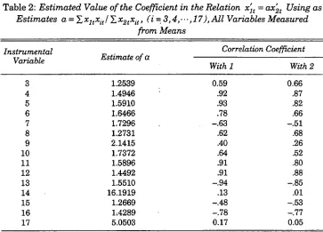
Table 2: Estimated Value of the Coefficient in the Relation x'lt = ax'2t Using as

Estimates a = £ xltxit /J,x2txit, (i = 3,4,--,17), All Variables Measured

from Means

Instrumental

Variable Estimate of a

Correlation Coefficient

With 1 With 2

3 1.2539 0.59 0.66

4 1.4946 .92 .87

5 1.5910 .93 .82

6 1.6466 .78 .66

7 1.7296 -.63 -.51

8 1.2731 .62 .68

9 2.1415 .40 .26

10 1.7372 .64 .52

11 1.5896 .91 .80

12 1.4492 .91 .88

13 1.5510 -.94 -.85

14 16.1919 .13 .01

15 1.2669 -.48 -.53

16 1-.4289 -.78 -.77

17 5.0503 0.17 0.05

V a r i a b l e s 1 a n d 2 constitute t h e investigational set. For the i n s t r u m e n t a l set w e have no fewer t h a n 15 series w h i c h Stone (op. cit., p. 11) n u m b e r s 3 to 17: t h e y need n o t be p a r t i c u l a r i z e d here. I n his Table I I Stone gives t h e complete variance-covariance m a t r i x for t h e 17 variables, as w e l l as t h e c o r r e l a t i o n coefficients (Table I I I ) . F r o m these t a b l e s Table 2 has been compiled w i t h o u t difficulty.

The correlation between variables 1 and 2 is very h i g h , namely 0.97. Since i n s t r u m e n t a l v a r i a b l e 4 is (practically) t h e v a r i a b l e most h i g h l y correlated w i t h variables 1 a n d 2 we use i t to determine the estimate of a. W e f i n d a = 1.4946. T o a p r o b a b i l i t y o f 1/10 (not to adopt too h i g h a s t a n d a r d ) t h e s a m p l i n g l i m i t s (using 2.26) are found to be

1.3337 < a < 1.7378,

w h i c h are far w i d e r t h a n t h e regression l i m i t s given by

(i) Xi = 1.3543 x2 (xi on x2) ,

(ii) X i = 1.4491 x2 ( x2 on X l) .

t h e varianceTCOvariance m a t r i x of xl t, xat, x3 t as determined b y the sample: if, i n p a r t i c u l a r , au, p , ^ , a n d |i22 are k n o w n , t h e n from Frisch's theorem (1934) we m u s t t a k e t h e regression l i m i t s as t h e absolute l i m i t s of a. A t t h e same t i m e w e m u s t recognize t h e a r b i t r a r y n a t u r e of t h e a s s u m p t i o n t h a t for so s m a l l a sample as 17 t h e variance-covariance m a t r i x should be regarded as given b y t h e data. U s i n g M . S . B a r t l e t t ' s theorem (1933) as t o t h e d i s t r i b u t i o n o f t h e S t u d e n t i z e d r e g r e s s i o n coefficient, we f i n d t h a t t h e r e g r e s s i o n coefficient ( i i ) g i v e n as 1.4491 m i g h t (on p r o b a b i l i t y 1/10) have come from a p o p u l a t i o n w i t h t h i s coefficient r a n g i n g f r o m 1.294 to 1.646, so t h a t a h i g h correlation is no guarantee of regression-coefficient s t a b i l i t y w h e n t h e sample is small.

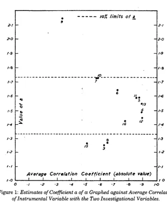
F i g u r e 1 based o n Table 2 shows clearly t h a t the h i g h e r t h e i n s t r u m e n t a l c o r r e l a t i o n , t h e m o r e t h e estimates t e n d to cluster a r o u n d t h e "true" figure w h i c h is;probably i n t h e neighbourhood o f 1.4-1.5. W h e n the correlations are i n s i g n i f i c a n t t h e e s t i m a t e s are fantastic. W h e n t w o i n s t r u m e n t a l variables are close together o n t h e d i a g r a m , or even w h e n t h e y t e n d t o give m u c h t h e same e s t i m a t e of a, u s u a l l y we f i n d t h e m h i g h l y correlated (from Stone's table). T h u s b e t w e e n 7 a n d 10 t h e c o r r e l a t i o n is - 0 . 9 0 , a n d 0.96 between 6 a n d 10, 0.98 b e t w e e n 5 a n d 1 1 , - 0 . 9 7 between 5 and 13. T h i s phenomenon is a r e m i n d e r t h a t , w h i l e close s i m i l a r i t y i n t w o or more estimates of a based on different i n s t r u m e n t a l variables m a y n o r m a l l y be regarded as good evidence t h a t t h e r e l a t i o n is complete ( i n a sense to be defined i n t h e next section) we s h o u l d be c h a r y about accepting i t i f t h e i n s t r u m e n t a l variables are h i g h l y correlated.

As far as t h e t e s t goes, i t does n o t c o n t r a d i c t t h e hypothesis t h a t t h e r e l a t i o n x 'l t = o<x2 t between the systematic p a r t s of t h e variables is complete. T h e t e s t i s , however, insensitive for so s m a l l a sample.

V I D E T E R M I N A T I O N A N D A S S E S S M E N T O F A C C U R A C Y O F C O E F F I C I E N T S I N E Q U A T I O N S I N T H E S Y S T E M A T I C PARTS

O F M O R E T H A N T W O V A R I A B L E S

2t

•

9

• io% limits of «_

21

2-0

-

2-0

rs

-

/•9

r-&

IO

/•8

h7

-

7 _1-7

1-6

r-s

o

•

6

5

•13

i

/ • €

l-S

1-4 ₁₆ • A? f4

1-3

1-2

8

* r

-1-3

1-2

/ . /

Average Correlation Coefficient (absolute value)

/ • /

1-0 I 1 I I i ' i i i I / O

[image:27.479.65.401.61.468.2]

O I -2 -3 -4 -S -6 -7 -6 9 IO

Figure 1: Estimates of Coefficient a of a Graphed against Average Correlation

of Instrumental Variable with the Two Investigational Variables.

Note: Numbers indicate i n s t r u m e n t a l variables as shown i n Table 2.

I n the equation the n u m b e r of variables may be

(i) j u s t enough, w h e n t h e equation is said to be complete; (ii) more t h a n sufficient, w h e n t h e equation is overdetermined; ( i i i ) too few, w h e n t h e equation is said to be incomplete.

reference t o i t s s a m p l i n g s t a n d a r d d e v i a t i o n , t h e f o r m u l a for w h i c h for large samples was g i v e n . I t m u s t be confessed i n practice t h a t t h e m e t h o d has p r o v e d a w k w a r d for c a l c u l a t i o n a n d i n s e n s i t i v e for inference, t h o u g h i n g r e a t e r or lesser degree i n s e n s i t i v i t y bedevils most tests o f significance o f economic t i m e series.

A n a l t e r n a t i v e m e t h o d t h a t seems more l i k e l y to y i e l d satisfactory r e s u l t s is t h e f o l l o w i n g . H a v i n g estimated the coefficients a, from (10), set

yt = £ « ixi t > (82)

i=l

t a k i n g t h e c a l c u l a t e d a; as e s t i m a t e s ( p r o p o r t i o n a t e l y ) o f t h e a;. T h e systematic p a r t s and t h e disturbances of yt are given by

y ; = i ai X;t,

1 ' (83)

y i = i < * ixi t >

i

t h o u g h these are, of course, u n k n o w n separately. L e t zt be a n i n v e s t i g a t i o n a l v a r i a b l e n o t i n c l u d e d i n t h e set xi t ( i = L 2, • • •, p). W r i t e

y't

= K

(84)

a n d l e t wt be a n i n s t r u m e n t a l v a r i a b l e n o t included i n t h e o r i g i n a l sets. W e are n o w i n exactly t h e s i t u a t i o n of previous sections for d e t e r m i n i n g w h e t h e r t h e coefficient P is s i g n i f i c a n t l y different from zero. The disturbances of yt, zt, wt m a y be deemed i n d e p e n d e n t i n t h e m a n n e r r e q u i r e d a n d t h e necessary variance-covariance m a t r i x of ( yt, zt, wt) can be estimated j u s t as was t h a t of (xi t > x2t> x3 t ) i n t h e previous section. I f t h e calculation (repeated i f possible a few times; u s i n g new functions zt a n d wt, each t i m e ) persists i n showing t h a t t h e e s t i m a t e b o f p i s n o t significant, t h e n t h e o r i g i n a l r e l a t i o n (2) m a y be deemed complete. T h i s m e t h o d c o u l d be used for t e s t i n g t h e v a l i d i t y o f

structural equations o f g i v e n form.

Case ( i i ) , t h a t o f over determination, w i l l be indicated by s m a l l values o f t h e coefficients o f one o r more o f t h e variables. H a v i n g purged t h e e q u a t i o n o f these d o u b t f u l v a r i a b l e s , one proceeds exactly as i n case ( i ) r e m e m b e r i n g , however, always t o use new variables, o f w h i c h one m u s t assume a n adequate supply o f t h e right k i n d .

v a r i a b l e is t h e n added to t h e r e l a t i o n w i t h t h e coefficient as d e t e r m i n e d a n d t h e process o f t e s t i n g t h e completeness of t h e new r e l a t i o n is repeated. Care m u s t be t a k e n to use, w h e n r e q u i r e d , new variables for t h e i n s t r u m e n t a l set.

W h e n t h e complete equation has been d e t e r m i n e d t h e s a m p l i n g l i m i t s o f each coefficient estimate m a y be f o u n d as follows, e.g., for ap/ a ! . W r i t e t h e r e l a t i o n i n t h e form

where

%£*+u't=0 (85)

ut = x i t+— x2 t + ••• +- J^x p - U (86)

ax ax

a n d f i n d t h e l i m i t s of a ^ u s i n g (36), again t a k i n g t h e computed a ^ as t h e values of aja^ i = 2, 3 , . . . , p - l

I t should be r e m a r k e d t h a t t h e test of significance proposed i n t h i s section for t h e several-variable case is exact o n l y w h e n t h e coefficient estimates are (proportionately) exactly equal to t h e 0Cj. A c t u a l l y , as we have seen, t h e e s t i ­ mates are subject to wide s a m p l i n g deviations unless t h e samples are v e r y l a r g e ; nevertheless they are consistent estimates w h i c h t e n d i n p r o b a b i l i t y t o w a r d s t h e p o p u l a t i o n values, and, w h i l e inferences as t o significance m a y be w r o n g o n account of s a m p l i n g errors of estimate o f t h e coefficients, t h e y w i l l be r i g h t i n t h e long r u n .

We have seen t h a t i n t h e case of two variables t h e accuracy of t h e estimate of t h e coefficient depends l a r g e l y o n t h e c o r r e l a t i o n o f t h e i n s t r u m e n t a l v a r i a b l e x3 t w i t h t h e i n v e s t i g a t i o n a l v a r i a b l e W h a t is t h e corresponding p r o p e r t y w h e n t h e n u m b e r o f i n v e s t i g a t i o n a l v a r i a b l e s exceeds two? F r o m (10) i t w i l l be seen t h a t t h e estimate a of t h e r a t i o o f a n y t w o coefficients a; m a y be expressed i n the form

a = r " / t/, (87)

w h e r e t h e elements of the t w o d e t e r m i n a n t s r ' and r " are t h e covariances mi r. I n t h e large-sample case a n d w i t h some o t h e r w i d e assumptions i t has been s h o w n (Geary, 1943) t h a t t h e confidence l i m i t s o f a c o r r e s p o n d i n g t o a p r o b a b i l i t y are given approximately b y t h e roots of t h e q u a d r a t i c e q u a t i o n ( i n a) (cf. (56)):

X2 ( g2a2 - 2g la + g0) = (X.2 p - 1 2 + n ) ( p ' a - p " )2, (88)

t h e n o r m a l p r o b a b i l i t y p o i n t corresponding to p r o b a b i l i t y n (e.g., w h e n n. = 0.05, X, = 1.96), g0, gi, g2 homogeneous q u a d r a t i c expressions i n t h e f i r s t m i n o r s o f p ' a n d p " o f f o r m specified i n t h e o r i g i n a l paper.

I t i s clear f r o m (88) t h a t generally t h e larger t h e value of p' t h e closer t h e values of t h e roots of t h e q u a d r a t i c equation, a n d t h e smaller t h e value of p' t h e m o r e dispersed these values are. Accordingly t h e i n s t r u m e n t a l set should be so w e l l diversified as t o give p' t h e greatest possible value. T h i s is w h y , as r e m a r k e d above, t h e e s t i m a t e s f o u n d u s i n g as i n v e s t i g a t i o n a l sets a p a r t i c u l a r series a n d t h e same series lagged or advanced say one t e r m , t h o u g h these m a y generally be h i g h l y correlated w i t h t h e i n v e s t i g a t i o n a l set, m a y y i e l d inefficient estimates of the coefficient a;, because they m a y give t w o closely s i m i l a r lines i n t h e p x ( p - l ) m a t r i x mi r.

V I I C O N C L U S I O N

The m e t h o d here o u t l i n e d w i l l c e r t a i n l y f u r n i s h consistent estimates o f t h e coefficients of r e l a t i o n s between systematic p a r t s a n d d e t e r m i n e t h e i r s a m p l i n g l i m i t s , a n d p r o v i d e t h e n u m b e r o f sets o f observations, i n v e s t i ­ g a t i o n a l a n d i n s t r u m e n t a l , i f t h e n u m b e r of observations is l a r g e enough. Classical regression t h e o r y on w h i c h confluence analysis so l a r g e l y depends, w i l l o n l y afford consistent estimates i n t h e almost t r i v i a l case o f no d i s ­ t u r b a n c e or i n w h i c h so m a n y v a r i a b l e s have been i n t r o d u c e d i n t o t h e e q u a t i o n ( i n r e l a t i o n to t h e n u m b e r o f observations) t h a t t h e f i t of t h e plane to t h e observations is v e r y close (as i n d i c a t e d by t h e m u l t i p l e - c o r r e l a t i o n coefficient). T h i s is e m p h a t i c a l l y not t o say t h a t confluence analysis has n o t a v a l u e for d e t e r m i n i n g j u s t t h e set of variables c o n s t i t u t i n g a complete set. Some progress has been made recently t o w a r d s c o n s t r u c t i n g large charts for o m n i b u s : use i n confluence analysis designed t o reduce, i f n o t l a r g e l y t o e l i m i n a t e , t h e t e d i u m o f m a k i n g a " t i l l i n g " anew for each investigation.

A c t u a l l y a l l t h e f a m i l i a r difficulties of collinearity, etc., encountered i n con­ fluence a n a l y s i s arise i n t h e t e c h n i q u e here discussed, b u t t h e y have a n e n t i r e l y d i f f e r e n t character. T h e y can a l l be resolved i f t h e v a r i a b l e s a n d observations are n u m e r o u s enough, whereas i n classical regression analysis, no m a t t e r h o w m a n y observations there are, the estimates of the coefficient are biased.

I t only r e m a i n s now to b u i l d u p a set of applications of the theory to test i t s p r a c t i c a l efficacy!

REFERENCES

BAETLETT, M.S., 1933. "On the Theory of Statistical Regression", Proceedings of the

Royal Society of Edinburgh, Vol. 53, p. 260.

CRAMER, H . , 1937. Random Variables and Probability Distributions, Cambridge Tracts i n Mathematics, No. 36, Cambridge.

FRISCH, R., 1934. Statistical Confluence Analysis by Means of Complete Regression

Systems, Universitetets 0konomiske Institutt, Oslo.

GEARY, R.C., 1930. T h e Frequency Distribution of the Coefficients of Two Normal Variates", Journal of the Royal Statistical Society, Vol. 93, Part I I I , pp. 442-446. GEARY, R.C., 1936. "Moments of the Ratio of the Mean Deviation to the Standard

Deviation for Normal Samples", Biometrika, Vol. 28, Parts I I I and IV, pp. 295-305. GEARY, R.C., 1942. "Inherent Relations between Random Variables", Proceedings of

the Royal Irish Academy, Vol. 47, A, 6, pp. 63-76.

GEARY, R.C., 1943. "Relations between Statistics: the General and the Sampling Problems when the Samples Are Large", Proceedings of the Royal Irish Academy, Vol. 49, A, 10, pp. 177-196.

GEARY, R.C., 1948. "Studies i n Relations between Economic Time Series", Journal of

the Royal Statistical Society, Series B (Methodological), Vol. 10, No. 1, pp. 140-158.

REIERS0L, O., 1941. "Confluence Analysis by Means of Lag Moments and Other Methods of Confluence Analysis", Econometrica, Vol. 9, No. 1, pp. 1-24.

REIERS0L, O., 1945. Confluence Analysis by Means of Instrumental Sets of Variables, Uppsala.

STONE, R., 1947. "On the Interdependence of Blocks of Transactions", Supplement to

the Journal of the Royal Statistical Society, Vol. 9, No. 1, pp. 1-45.

TINTNER, G., 1945. "A Note on Rank, Multicollinearity and Multiple Regression",