Testing the exogeneity assumption in panel data models with "non classical" disturbances

Department of Economics University of Southampton Southampton SO17 1BJ UK

Discussion Papers in

Economics and Econometrics

TESTING THE EXOGENEITY ASSUMPTION IN PANEL DATA MODELS WITH

“NON CLASSICAL” DISTURBANCES

Raymond O’Brien Eleonora Patacchini

No. 0302

Testing the Exogeneity Assumption in Panel Data

Models with “Non Classical” Disturbances

Raymond O’Brien

Eleonora Patacchini

University of Southampton

February 20, 2003

Abstract

This paper is concerned with the use of the Durbin-Wu-Hausman test for correlated effects with panel data. The assumptions underlying the construc-tion of the statistic are too strong in many empirical cases. The consequences of deviations from the basic assumptions are investigated. The size distortion is assessed. In the case of measurement error, the Hausman test is found to be a test of the difference in asymptotic biases of between and within group estima-tors. However, its ‘size’ is sensitive to the relative magnitude of the intra-group and inter-group variations of the covariates, and can be so large as to preclude the use of the statistic in this case. We show to what extent some assumptions can be relaxed in a panel data context and we discuss an alternative robust formulation of the test. Power considerations are presented.

Keywords: models with panel data, Hausman test, minimum variance esti-mators, quadratic forms in normal variables, Monte Carlo simulations

1

Introduction

The Hausman test is the standard procedure used in empirical work in order to discriminate between the fixed effects and random effects model. It can be described as follows.1

Suppose that we have two estimators for a certain parameterθof dimensionK_×1.

One of them , bϑr, is robust, i.e. consistent under both the null hypothesis H0 and the alternativeH1, the other,bϑe,is efficient and consistent underH0 but inconsistent under H1. The difference between the two is then used as the basis for testing. It can be shown (Hausman, 1978) that, under appropriate assumptions, under H0 the statistich based on³ϑbR−bϑE

´

has a limiting chi-squared distribution:

h=³ϑbr−ϑbe

´0h

d

V ar³bϑr−bϑe

´i−1³

b

ϑr−bϑe ´ _a

∼χ2k.

If this statistic lies in the upper tail of the chi-square distribution we reject H0. If the variance matrix is consistently estimated, the test will have power against any alternative under which bϑr is robust and bϑe is not. Holly (1982) discusses the power

in the context of maximum likelihood.

In a panel data context the test can be used as a test for correlated effects. The null hypothesis assumes lack of correlation between the individual effect ηi and

explanatory variablexit :

H0 :Cov(xit,ηi) = 0.

The Within Groups estimator, bβwg, is robust regardless of the correlation betweenηi

and xi. The Balestra-Nerlove estimator, bβBN, is efficient under H0 but inconsistent under H1 :

H1 :Cov(xit,ηi)6= 0.

The Hausman statistic in this case takes the form

h1 =

³ b

β_wg−bβ_BN´0hV ard ³bβ_wg−βb_BN´i−1³βb_{wg −}bβ_BN´_∼a χ2_k. (1)

If we cannot reject the null hypothesis then the most reasonable model for the data at hand is the random effects model, otherwise the fixed effects model is more justified. However, using the results in Hausman (1978), the statistic used in practice

h2 =

³ b

βwg −bβBN ´0³

b

Vwg−VbBN

´−1³

b

βwg −βbBN ´

, (2)

where Vwg = V ar ³

b

βwg ´

and VBN =V ar ³

b

βBN ´

. It is based on the result that the variance of the difference between an estimator and an efficient estimator is equal to

1_{This approach is also used by Durbin (1954) and Wu (1973). For this reason tests based on the}

the differences of the variances:

V ar³bβ_wg−βb_BN´=Vwg−VBN. (3)

In the time series-cross section model considered in Hausman (1978) this equality holds because βbBN is an efficient estimator in the sense that it attains the

Cramér-Rao Lower Bound for fixed λ (defined below), and Cov³bβwg,bβBN ´

= V ar³βbBN ´

. This implies

V ar³βbwg−bβBN

´

= V ar³bβwg ´

+V ar³βbBN ´

−2Cov³bβwg,βbBN ´

= V ar³bβ_wg´+V ar³βb_BN´₋2V ar³βb_BN´

= V ar³bβ_wg´₋V ar³βb_BN´=Vwg −VBN.

However, in applied studies, this may not always be the case and one should be careful in usingh2 automatically. If equality (3) does not hold, h2 does not follow an asymptotic chi-squared distribution, even underH0.

This paper considers the effects on the Hausman statistic used in applied panel data studies,h2, of deviations from the conditions required in Lemma 2.1in Hausman (1978), which guarantees that equality (3) holds. The lemma is stated as follows.

Lemma 1 Consider two estimatorsβb₀, bβ₁ which are both consistent and asymptot-ically normally distributed with βb0 attaining the asymptotic Cramér-Rao bound so that √T ³βb0 −β

´ _a

∼N(0, V0) and√T ³bβ1−β

´ _a

∼N(0, V1) where V0 is the inverse of Fisher’s information matrix.Consider_bq=bβ1−βb0. Then the limiting distributions of √T ³βb₀₋β´ and√T_bq have zero covariance,Cov³βb₀,q_b´= 0, a null matrix.

The plan of the paper is as follows.

Regarding the attainment of the Cramér-Rao Lower Bound, in Section 2 we prove that if we want to compare different estimators within a specific set, the assumption of full efficiency is not necessary. A relative lower bound for the variance can play the role. The variance of the difference between two estimators belonging to such a set is still equal to the difference of the variances if one of the two is the minimum variance estimator in the specific set considered. The algebraic derivation of this result is provided in the panel data framework. The Lemmas contained in Appendix 1 prove that this holds both in the exact and in the limiting case. Given that the Balestra-Nerlove estimator can be obtained as a matrix weighted average of the Between Groups, βbbg, and the Within Groups estimators (Maddala, 1971), we consider the

However, even the attainment of a minimum variance bound may be a strong assumption in empirical studies. This circumstance is related to assumptions about the error term. A failure of the assumption of spherical disturbances is quite common circumstance in practice. Section 3 presents a robust formulation of the Hausman test for correlated effects, which is based on the construction of an auxiliary regression. We explain and discuss to what extent the use of artificial regressions may allow us to construct tests based on the difference between two estimators in a panel data model without making strong assumptions about the disturbances. The motivation underlying the implementation of the robust test is that the size distortion of the standard Hausman test, h2, in cases of misspecification of the variance-covariance matrix of the disturbances may be serious. This is investigated in Section 5.

The failure of the consistency of the two estimators under the null is discussed in Section 4. Such discussion is extremely relevant because a possible failure of the consistency of theWithin Groups and theBalestra-Nerlove estimators,not related to the source of endogeneity being tested, is almost never raised in empirical studies. We explain to what extent the econometrics of panel data, offering a variety of different estimators for the same parameter, can help us to deal with this issue.

Section 6 compares the power of the standard Hausman test and the robust formu-lation presented in Section 3 using a Monte Carlo experiment. Section 7 concludes.

2

The Failure of the Assumption of Full E

ffi

ciency

Consider the following model

yit =x

0

itβ+ηi+vit, i= 1, ..., N, t = 1, ..., T (4)

where xit is a K×1 vector of stochastic regressors, ηi ∼ iid ¡

0,σ2

η ¢

, vit ∼iid(0,σ2)

are uncorrelated with xit andCov(ηi, vit) = 0.

Defining the disturbance term

εit =ηi+vit,

the variance-covariance matrix of the errors is

Σ (N T×N T)

=IN ⊗Ω

where

Ω=

  

σ2η+σ2 . . . σ2η

..

. . .. ... σ2

η . . . σ2η+σ2

 

=σ2IT +σ2η ιι

0

(5)

andι is a column vector ofT ones.

Hausman and Taylor (1981) propose three different specification tests for the hypothesis of uncorrelated effects: one based on the difference between the Within Groups and the Balestra-Nerlove estimator, another on the difference between the Balestra-Nerlove and the Between Groups and a third on the difference between the Within Groups and the Between Groups. They show that the chi-square statistics for the three tests are numerically identical. We now analyze the Hausman statistic constructed on the difference between the Within Groups and the Balestra-Nerlove estimator, commonly used in empirical work.

Hereafter, we define as fully efficient an estimator that reaches the Cramér-Rao Lower Bond and as minimum variance the one that has the minimum variance within a specific class. Let

λ= σ

2

σ2 _+Tσ2

η .

If we assume normality in model (4), it is well-known that the Balestra-Nerlove esti-mator, i.e. the generalized least square estiesti-mator, is fully efficient if the variance-ratio parameterλis known, and asymptotically fully efficient ifλis consistently estimated. (A distributional assumption is required in order to obtain the Cramér-Rao Bound.) Therefore the hypothesis underlying the construction of the Hausman statistic are satisfied and the results of the test are reliable. However, we will demonstrate that even without assuming normality of theεit the results of the standard Hausman test

are reliable, the key assumption being (5). We will use the panel data framework as an example. In what follows we takeλ as known. The same result holds asymptotically if a consistent estimator bλ is available. It is implied by the Hausman-Taylor result that we can construct the same test usingβb_wg andβb_bg,as will be clarified below.

We write the Balestra-Nerlove estimator (Balestra and Nerlove, 1966) as a func-tion of the variables in levels

b

β_BN =³X0QX +λX0M X´−1³X0Q+λX0M´Y (6)

where

Q = IN ⊗Q+,

Q+ = IT −

1

Tii

0

,

M = IN ⊗M+,

M+ = 1

Tii

0

=IT −Q+,

X =      X1 X2 .. . XN    

, Y =

     y1 y2 .. . yN    

, Xi =

     x0 i1

x0i2 .. . x0 iT    

, yi =

    

yi1

Q+ is the matrix that transforms the data to deviations from the individual time mean, M+ _{is the matrix that transforms the data to averages. Rearranging}

b

β_BN =hX0[λIN T + (1−λ)Q]X i−1

X0[λIN T + (1−λ)Q]Y. (7)

The variance is

V ar(bβBN) =

½h

X0[λIN T + (1−λ)Q]X

i−1

X0[λIN T + (1−λ)Q]

¾

V ar(Y)

×

½

[λIN T + (1−λ)Q]X h

X0[λIN T + (1−λ)Q]X

i−1¾

. (8)

Using a simplified version of the Sherman-Morrison-Woodbury formula (Golub and Loan, 1983, p.50) one can show, that, under assumption (5), the variance of yi can

be written as2

V ar(yi) = σ2

·

IT −

σ2η

σ2_+Tσ2

η

ιι0

¸−1 =σ2

·

IT −

1

T(1−λ)ιι

0¸−

1

= σ2

·µ

IT −

1

Tιι

0¶

+λ1

Tιι

0¸−

1

.

This can also be obtained by ignoring time effects, and thus settingω= 0,in Nerlove (1971). Using the matrices involved in formula (6), we can rewrite this expression as

V ar(yi) = σ2

£¡

IT −M+

¢

+λM+¤−1 (9)

= σ2£Q++λIT −λQ+ ¤−1

(10)

= σ2£λIT + (1−λ)Q+ ¤−1

. (11)

Thus

V ar(Y) =IN ⊗V ar(yi) =σ2[λIN T + (1−λ)Q]−1.

Substituting (11) in (8), we obtain

V ar(bβ_BN)

= σ2hX0[λIN T + (1−λ)Q]X i−1

X0[λIN T + (1−λ)Q] [λIN T + (1−λ)Q]−(12)1

×[λIN T + (1−λ)Q]X h

X0[λIN T + (1−λ)Q]X

i−1

= σ2

h

X0[λIN T + (1−λ)Q]X

i−1

. (13)

Similarly, using theQmatrix defined in formula (6), we write also theWithin Groups estimator as a function of the initial variables in levels

b

βwg= h

X0QXi−

1

X0QY. (14)

The variance is

V ar(bβ_wg) =hX0QXi−1X0Q(V arY)Q0XhX0QXi−1. (15)

If we transform the data into deviations, the variance ofyi can be written as

V ar(Q+yi) =Q+V ar(yi)Q+

0

=σ2Q+hIT +θιι

0i

Q+ =σ2Q+Q+ =σ2Q+ (16)

where θ=σ2η/σ2 and Q+ι= 0,a vector of zeros. Thus

V ar(QY) =σ2IN ⊗Q+=σ2Q

Plugging (16) in (15), we obtain3

V ar(bβ_wg) = σ2hX0QXi−1X0QQQ0XhX0QXi−1

= σ2hX0QXi−1. (17)

Hence, from (13) and (17)

V ar(βbwg)−V ar(bβBN) =σ2

½h

X0QXi−

1

−hX0[λIN T + (1−λ)Q]X i−1¾

. (18)

Next we show that such expression is exactly equal to the variance of the difference between the two estimators.

V ar(bβBN −bβwg) =V ar(βbBN)−Cov(βbBN,βbwg)−Cov(βbwg,βbBN) +V ar(bβwg).

>From (7) and (14)

Cov(bβBN,bβwg)

= σ2hX0[λIN T + (1−λ)Q]X i−1

X0[λIN T + (1−λ)Q]

×[λIN T + (1−λ)Q]−1QX h

X0QXi−

1

= σ2hX0[λIN T + (1−λ)Q]X i−1

=V ar(βb_BN).

This is symmetric, and thus equal to Cov(bβ_wg,βb_BN). Thus using (11) and (16), we obtain

V ar(βbBN −βbwg) = V ar(bβBN)−V ar(βbBN)−V ar(bβBN) +V ar(βbwg) (19)

= V ar(bβ_wg)₋V ar(bβ_BN)

as required. We have proved that equality (3) holds for λ known or otherwise fixed. As we said, the case of estimated λ can be treated by using the Hausman-Taylor result that an algebraically identical test statistic can be constructed using the dif-ference between bβwg and the Between Groups estimator bβbg. We obtain

(bβ_wg−βb_bg)0hV ar(bβ_wg) +V ar(bβ_bg)i−1(βb_wg−bβ_bg)

as the estimators have zero covariance. In this form, we can see that estimating σ2 _{and λ (or σ}2

η) affects only the variance matrix of the test statistic. We thus

obtain the same test statistic whatever λ is, and (2) remains correct. It does not follow from these arguments that the equality (3) can be made exact for estimated λ. If bβ_BN and bβ_wg were independent of λb, the result would follow, but this requires normality of the disturbances. Viewing bβ_BN as a feasible GLS estimator, Kakwani (1967) implies it is unbiased. However, conditional on bλ it may or may not be unbiased. Further, the variances obtained are for λ fixed, not conditional on λb. So attempts to obtain unconditional variances from conditional variances and variances of conditional expectations do not seem fruitful. So it would appear that the exact result (3) may require normality of theεitorλfixed. Equality (3) implies that forfixed

and knownλ,and knownσ2_{,under normality hwould have an exactχ}2 _{distribution.} If λ is estimated, and/or the εit are not normal, h is asymptotically χ2 as long

as xit are sufficiently well-behaved to ensure that βbBN and βbwg are asymptotically

normal, and σ2 _{and σ}2

η (or equivalently λ) are appropriately estimated. This is less

restrictive than the assumptions required for the identification of the Cramér-Rao bound. We obtain the result (3) without assuming normality because we compare two linear unbiased estimators, one of them achieving the minimum variance for a linear estimator. Lemma 4 in Appendix 1 shows that the variance result depends only on minimum variance properties, not on normality or achievement of a particular (Cramér-Rao) bound. However, in order to get a panel data generalized version of Lemma 1, it is necessary to prove a similar result in the limiting case. This aim is achieved in Lemma 10 in Appendix 1. The minimum variance property required is within a set of the form

T ={t:t=At1+ (I−A)t2}

where t1 andt2 are estimators of the parameter vector θ. For completeness, Lemma 9 establishes that sets of this form will contain minimum variance members.

for the variance can play the required role. The variance of the difference between two estimators belonging to the same set is still equal to the difference of the variances if one of the two is the minimum variance estimator in the specific set. Lemma 10 in Appendix 1 allows us to rely on the results provided by a traditional Hausman test in a more general set-up.

It is worth noting that we are not removing the assumption of asymptotic normal-ity of the estimators in Lemma1, which is needed to obtain theχ2 distribution of the Hausman statistic. Our generalization applies for estimators that are asymptotically normally distributed but that do not reach the Cramér-Rao Bound.

We prove the result for a specific set of estimators but this does not rule out the possibility of extending the result to wider contexts. For instance, the GMM estimator is asymptotically normally distributed and attains the asymptotic Cramér-Rao Lower Bound only in some cases. Nevertheless, if we compare an arbitrary GMM estimator, e.g. using the identity matrix, and the one which uses the optimal weighting matrix (Hansen, 1982), Lemma 10 implies that Hansen’s GMM can be used as basis for a Hausman test.

3

The Failure of the Assumption of Spherical

Dis-turbances

In the previous section, we relaxed the assumption of full efficiency in Lemma 1. However, even the assumption that one of the two estimators has the minimum variance or that both are consistent under the null hypothesis can be still too strong in many empirical cases. In the panel data framework above considered (model (4)), the crucial assumption for (3) to hold is (5). In other words, the form of the covariance matrix has to be assumed. In cases of misspecification, i.e. if V ar(y) = Ω∗ _{6= Ω,}

equality (3) does not hold any longer.

As Hausman clearly states at the very beginning of his article (Hausman, 1978), the specification test he presents takes the hypothesis that the disturbances have a spherical covariance matrix. He considers the standard regression framework

y=Xβ+ε, (20)

where

E(ε/X) = 0, (21)

and

V ar(ε/X) = σ2I. (22)

In most of the articles that followed, assumption (22) is never relaxed. The empha-sis of this part of literature is placed in testing the orthogonality assumption, i.e.

The reason is straightforward if we consider the comparison between the Within Groups estimator and the Balestra-Nerlove estimator as a comparison between an OLS and aGLS estimator. One basic assumption in the construction of the Hausman statistic (Lemma 2.1 in Hausman, 1978) is that one of the two estimators has to reach the asymptotic Cramér-Rao Lower Bound or, using the generalization provided in Lemma 4 in Appendix1, that at least has to be the minimum variance estimator in a specific class. In the panel data framework the Balestra-Nerlove, that is the generalized least square estimator, is the BLUE estimator if theGLS transformation produces spherical disturbances. This is the case if the correlation in the covariance matrix of the initial errors is due only to the omission of the individual effects, i.e. if the initial disturbances are spherical.

To make it clear, we analyze in detail the construction of the Balestra-Nerlove estimator. In practice the Balestra-Nerlove estimator can be calculated running an OLS regression on a transformed model. Assuming model (4), which implies the disturbances variance covariance matrix (5), the transformation of theyi and the xi

is the following

Ω−12y

i =     

yi1−θyi.

yi2−θyi.

.. .

yiT −θyi.

    

where

Ω−12 =I− θ

Tii

0

, θ= 1_{− ¡} σ

σ2_+Tσ2

η ¢1

2

and likewise for the rows of xi.

Under assumption (5), which implies initial spherical disturbances, this is a GLS transformation that produces a model with spherical disturbances. Hence running OLS on such a model we obtain the BLUE estimator. However, if assumption (5) does not hold, theGLS transformation does not guarantee that the new disturbances are spherical. In this case the GLS estimator, namely the Balestra-Nerlove, is still consistent but it may not be the minimum variance estimator. The consequence is that we can no longer be sure that the equality (3) still holds. In these circumstance the results of the test may not be reliable. However, if the two estimators remain consistent the comparison can still be conducted, but the methodology needs to be adjusted in an appropriate way.

pro-vides estimators for the variances that are consistent and robust to heteroskedasticity and/or serial correlation of arbitrary form in the covariance matrix of the random disturbances. These estimators are obtained using White’s formulae (White, 1984). It will be made clear to what extent the application of White’s heteroskedasticity con-sistent estimators of covariance matrices in a panel data framework may also allow for the presence of dynamic effects.

Different artificial regressions have been proposed in the panel data literature to test for the presence of random individual effects, such as a Gauss-Newton regression by Baltagi (1996) or that proposed by Ahn and Lo (1996). However, the assumption of initial spherical disturbances has not been relaxed. As shown by Baltagi (1997, 1998), under the assumption of spherical disturbances, the three approaches, i.e. the Hausman specification test, the Gauss-Newton regression and the regression proposed by Ahn and Lo, yield exactly the same test statistic. Arellano (1993) first noted in the same panel data framework that an auxiliary regression can also be used to ob-tain a generalized test for correlated effects which is robust to heteroskedasticity and correlation of arbitrary forms in the disturbances. Davidson and MacKinnon (1993) list at leastfive different uses for artificial regressions including the calculation of esti-mated covariances matrices. We will use this device to estimate directly the variance between the two estimators without using equality (3). Furthermore, the application of White’s formulae (White,1984) in the panel data case will lead to heteroskedastic-ity and autocorrelation consistent estimators of such variance. Therefore, we can use an artificial regression to construct a test for the comparison of different estimators which is robust to deviations from the assumption of spherical disturbances. From now on we will call this technique the HR-test, for Hausman-Robust test.

Next we present the auxiliary regression that was proposed by Arellano (1993) to test for random versusfixed effects in a static panel data model.

Consider the general panel data model for individual i

yi

(T×1) = Xi

(T×K)

β+ vi

(T×1)

, i= 1, ..., N.

This system of T equations in levels can be transformed into (T ₋1) equations in deviations and one in averages. We obtain

½

y∗

i =x∗iβ+µ∗i −→(T −1) equations yi =xiβ+µi −→ 1 equation.

Estimating byOLS theN(T₋1)equations in orthogonal deviations from individual time-means we obtain the Within Groups estimator, i.e. βb_wg. Estimating by OLS theN average equations we obtain theBetween Groups estimator, i.e.βbbg.

Let

β_wg =E³bβ_wg´

and

Rewrite the system as

½

y∗i =x∗iβwg+µi∗−x∗iβbg+x∗iβbg

yi =xiβbg +µi.

Rearranging, we obtain

½

yi =x∗i

¡

βwg−βbg ¢

+x∗iβbg+µ∗i

yi =xiβbg +µi.

Call

Y_i+ =

µ

y∗

i yi

¶

, W_i+ =

µ

x∗

i x∗i

0 xi ¶

,

β+=

µ

β₁ β2

¶

=

µ

β_wg−β_bg βbg

¶

, µ+_i =

µ

µ∗

i µi

¶ .

The augmented auxiliary model is

Y_i+=W_i+β++µ+_i , i= 1, ..., N. (23)

If we estimate β+ by OLS, we obtain directly the variance of the difference of the two estimators in the upper left part of the variance-covariance matrix of β+. If we then estimate this covariance matrix using the White’s formulae and we perform a Wald test on appropriate coefficients, we obtain a reliable HR-test comparing the two estimators we are interested in, namely bβ_wg andβb_bg. Asfirst noted by Arellano (1993), under the assumption of spherical disturbances a Wald test on appropriate coefficients in the auxiliary regressions is equivalent to the standard Hausman test. Appendix 4 provides an analytical derivation of this result. The following Lemma is proved.

Lemma 2 Given model (23),

b

β₁ =βb_{wg −}bβ_bg, (24)

V ar(bβ1) = V ar

³ b

βwg −βbbg ´

, (25)

An appropriate estimator V ard(βb₁) consistently estimates V ar(bβ₁). (26)

It is shown that, in order to get a consistent estimate of the variance, the first set of equations has to be scaled.

further assumptions, i.e. cross-sectional heteroskedasticity which takes on a finite number of different values.

Consider a simple panel data framework without fixed effects

yi1 =βxi1+εi1

yi2 =βxi2+εi2,

.. .

yiT =βxiT +εiT, i= 1, ..., N,

where

E(²i²

0

i) =   

σ2 _{. . . 0}

..

. . .. ...

0 . . . σ2

 

=σ2IT =Σ.

Assume that in the complete model

Ω (N T×N T)

=I_⊗Σ=

    

Σ 0 . . . 0

0 Σ ... ... ..

. ... . .. 0

0 . . . 0 Σ

   

. (27)

Define

Xi =

  

xi1 .. . xiT   

(T×1)

yi =

  

yi1 .. . yiT   

(T×1)

²i =

  

εi1 .. . εiT   

(T×1)

and rewrite the model as

yi

(T×1) =Xiβ

(T×1) + ²i

(T×1)

, i= 1, ..., N. (28)

This formulation allows us to consider panel data in the framework defined in White (1984). If we assume no cross-sectional correlation and N _{→ ∞}, all the hypotheses underlying the derivation of White’s results are satisfied. Hence, Proposition 7.2 in White (1984, p. 165) applies.

b

Σ=N−1 N X

i=1

b ²i²bi

0 p

−→Σ (29)

and

b

Ω=I _⊗Σb _−→p Ω.

obtain a consistent estimator of the whole matrix Σ. Hence, by applying the result (29) in the panel data case we obtain a consistent estimator of the variance covariance matrix of the disturbances that also allows for the presence of dynamic effects within groups.

Therefore, the estimators of the variance of the OLS estimators of β in the panel data model (28) can be obtained by

\

V ar(β) =

" _N X

i=1

³ Xi0Xi

´#−1 _XN

i=1

Xi0ΩbXi " _N

X

i=1

³ Xi0Xi

´#−1

. (30)

As stated by Arellano (1993), they are heteroskedasticity and autocorrelation consis-tent. Such estimators are the ones used in the implementation of the HR-test. This case is referred in White (1984) ascontemporaneous covariance estimation.

However, White (1984) also implements consistent estimators in another case that explicitly takes into consideration a grouping structure of the data. Consider again the panel data model (28). Replace assumption (27) by

Ω (N T×N T)

=

    

Σ1 0 . . . 0

0 Σ2 ... ... ..

. ... . .. 0

0 . . . 0 ΣN

   

.

In this context, in a slightly different notation from that used by White (1984, p.172-173), suitable for the panel data framework, we can obtain consistent estimators of the covariance matrixΩ using

b

Ω=diag(Σ1b ,Σ2b ,. . .ΣbN)

where

b

Σi =T−1²bi²bi0.

In other words, a consistent estimator for the covariance matrix of group i is constructed by averaging the group residuals over only the observations in group i.

In the balanced panel data case, their number is constant between groups and equal to T. This estimator is not only robust to autocorrelation of arbitrary form within groups but it also allows for the possibility that individual error covariance matrices may differ according to observable characteristics (such as region, union, race, etc....).

4

The Failure of the Orthogonality Assumption

between Regressors and Random Errors

This section refers to the use of the test in circumstances where even the con-sistency of the estimators under the null hypotheses cannot be assured. A possible failure of the consistency of the two estimators, not related to the source of endo-geneity being test, is almost never considered in empirical studies. It is worthwhile noting that the question addressed by the Hausman test is whether the parameters of interest have been estimated consistently. Thus, the test detects the presence of any possible endogeneity problem (Davidson and MacKinnon, 1989), not necessarily induced by a correlation between the regressors and the individual effects. Rejection may be also caused, for instance, by the presence of measurement errors-in-variables. Almost always in the widespread use of the Hausman test for correlated effects in static panel data modelling, the consistency of the Within Groups and the Balestra-Nerlove estimators under the null is not questioned. However if for instance we are in presence of measurement errors-in-variables, least square estimators do not lose only their efficiency but also their consistency. Our claim is that in such contexts the use of the standard Hausman test is not correct. In the presence of arbitrary measurement errors-in-variables, if we compare theWithin Groups estimator and the Balestra-Nerlove estimators to test for uncorrelated individual effects, we may be comparing two inconsistent estimators. Moreover, theWithin Groups estimator and theBalestra-Nerlove estimator areOLS estimators constructed on different transfor-mations of the data. Measurement errors can have different impact using different transformations of the data. For instance, if we use first differences the bias can be magnified (Griliches and Hausman,1986). As a consequence, the probability limits of two estimators calculated on different transformations of the data may be different. In this case the null distribution of the Hausman test will depend on this difference, and thus on the (unknown) parameters. In other words, in presence of measurement errors-in-variables the widespread practice of using the standard Hausman statistics based on the comparison between the Within Groups and theBalestra-Nerlove esti-mator is not methodologically correct and it can lead to unreliable results.

caused by correlation between regressors and individual effects. It is based on the use of appropriate HR-tests in a particular sequence.

5

The Size of the Test

In this section we investigate the size distortion which occurs in the use of the standard Hausman test when the basic assumptions (Lemma 2.1 in Hausman 1978) are not satisfied.

Consider the panel data model (4) presented in Section 3. The Hausman test investigates the presence of specification errors of the formE(ηi|xit)6= 0.The robust

version proposed in Section 3 tests such orthogonality assumption between explana-tory variables and disturbances in presence of other forms of misspecification. In particular we are interested in a possible misspecification in the variance-covariance matrix of the disturbances arising, for instance, from the presence of measurement errors in variables. This case may be the rule rather than the exception in applied studies.

We want to test the hypothesis

Ho :E(εit|xit) = 0 (31)

against the alternative

H1 :E(εit|xit)6= 0,

when

V ar(εi|xit)6=Ωi. (32)

Hausman (1978) shows that underHo the test statistic

h=q_b0Vb(_bq)−1q_b∼χ2k (33)

where, V(_bq) is the asymptotic variance of q, andk is the length of q. The same test statistic is obtained if we consider the vectorq_bequal to

b

q1 = (βbwg −bβBN),

orq_b2 = (βbbg −bβBN),

orqb3 = (βbwg −bβbg).

As Hausman and Taylor (1981) pointed out they are all nonsingular transforma-tions of one another. The estimate of the variance covariance matrix used in the three cases is

b

V(qb1) = Vb(βbwg)−Vb(bβBN),

orVb(q_b2) = Vbβbbg)−Vb(bβBN),

If we are in presence of misspecification of the form (32), none of the above expressions gives a consistent estimate of the variance-covariance matrix, even under

Ho. The distribution of the test statistic under Ho need to be investigated. The

nominal size may be quite different from the observed one.

To investigate the size distortion under normality, we use the distributions of quadratic forms in normal random variables.4 _{In particular, we use the following}

Lemma.5

Lemma 3 (in Lemma 3.2 in Vuong, 1989). Let x _∼ NK(0, V), with rank (V) ≤ K, and let A be an K _×K symmetric matrix. Then the random variable x0Ax is distributed as a weighted sum of chi-squares with parameters (K,γ), where γ is the vector of eigenvalues of AV.

This implies thatx0_Axisχ2

r,where r=rank(A), if and only if AV is idempotent

(Muirhead, 1982, Theorem1.4.5).

If A =V−1_{, i.e. in cases of no misspecification, AV is idempotent. The theorem} is satisfied and result (33) holds. The test statistic gives correct significance levels.

If A₆=V−1 but AV is idempotent then rank(A)< K and/orrank(V)< K but still (33) holds. We omit this case for simplicity of exposition.

If A₆=V−1 _{andAV is not idempotent, implying that the eigenvalues ofAV are} not 0 or 1, the asymptotic distribution of the Hausman test under Ho is a weighted

sum of central chi-squares

h_∼

K X

i=1

dizi2

where zi2 ∼ χ21 and di are the eigenvalues of AV. This implies that the significance

levels of the standard Hausman test are not correct.

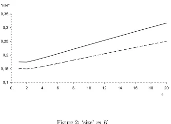
Consider first the limiting case where d1 → K, di → 0, i = 2, .., K. Figure 1

illustrates numerically that

Pr£Kχ2₁ >χ2_K,α¤,

where χ2K,α is the critical value for a test of sizeα under the χ2r distribution. In this

illustration α is set equal to 0.05.

In general we distinguish two effects: a scale effect if

K P i=1

di 6= K, which is

pre-dictable (e.g. if di = 2 ∀ i, h ∼ 2χ2K) and a dispersion effect if di 6= dj, even if K

P i=1

di =K. We normalize the weights and we conjecture that the dispersion effect is

maximized in the limit if we put all the weight on the largest eigenvalue, say thefirst one.

4_{See, among others, Murihead (1982, Ch. 1), Johnson and Kotz (1970, Ch.29).}

5_{Both this Lemma and the following one hold also in the asymptotic case (using the Continuous}

0 0.05 0.1 0.15 0.2 0.25

1 2 3 4 5 6 7 8 9 10 11 12 13 14 15 16 17 18 19 20

K "size"

Figure1: Pr£Kχ2

1 >χ2K,α ¤

Figure 1 illustrates this case, i.e. the tail area of a χ2

K is compared with the

maximum tail area of Kχ21.The graph shows that the size distortion is an increasing function ofK. For instance, ifK is equal to 14, an inappropriate use of the Hausman test will give a probability of rejecting a true hypothesis of exogeneity which is almost 4 time larger than the nominal size.

In certain simple contexts an expression for the eigenvalues of AV can be ana-lytically derived. For instance, a common source of misspecification in the variance covariance matrix occurs when elements of the regressor matrix contain measurement errors.

Suppose the true model is

yit =z

0

itβ+ηi+vit, i= 1, ..., N, t= 1, ..., T (34)

where z_it0 is a 1_×K vector of theoretical variables, ηi ∼ iid ¡

0,σ2

η ¢

, vit ∼ iid(0,σ2)

uncorrelated with the columns ofzit andCov(ηi, vit) = 0.The observed variables are

xit =zit+mit,

where mit is a vector of measurement errors uncorrelated with ηi and vit. The

esti-mated model is

yit =x

0

In the case of exact measurement, i.e. mit = 0,

V ar(yit) = E(ηi +vit)2 =σ2η +σ

2_,

Cov(yit, yit−s) = Cov(x

0

itβ+ηi+vit, x

0

it−sβ+ηi+vit−s)

= σ2η ∀s.

The variance-covariance matrix is matrix (5). It can be written as

Σ (N T×N T)

=IN ⊗Ωi,

where

Ωi =σ2IT +σ2η ιι

0

=σ2[IT +ϑ1ιι

0

], (36)

and

ϑ1 = σ

2

η

σ2. If we assume that mit ∼iid(0,ΣM), we obtain

V ar(yit) = E(ηi+vit−βmit)2 =σ2η +σ

2_+β0_Σ Mβ,

Cov(yit, yit−s) = Cov(x

0

itβ+ηi+vit−β0mit, x

0

it−sβ+ηi+vit−s−β0mit−s)

= σ2η ∀s6= 0.

So

Ωi = ¡

σ2+β0ΣMβ ¢

IT +σ2η ιι

0

=¡σ2+β0ΣMβ ¢

(IT +ϑ2ιι

0

), (37)

and

ϑ2 = σ

2

η

σ2_+β0_Σ Mβ

.

Consider now the exogeneity test based, for instance, on the comparison betweenβbBG

andbβ_{W G}. In this case, the measurement errors renderβb_BG andβb_{W G} inconsistent. If we assume that

plim(bβ_BG−β) =plim(βb_{W G−}β) = [ΣZQZ/(T −1) +ΣM]−1ΣMβ = [ΣZM Z+ΣM]−1ΣMβ

we show in Appendix 5 that if the rows Mi vN ID(0,ΣM) √

N(bβW G−bβBG)

D

→N(0,[1/(T ₋1)_}[ΣZQZ/(T −1) +ΣM]−

1 ×

£

(σ2+β0ΣMβ)ΣZQZ/(T −1) +σ2ΣM +{ΣMββ0ΣM + (β0ΣMβ)ΣM} ¤

× [ΣZQZ/(T −1) +ΣM]−

1

+ [ΣZM Z +ΣM]−

1 ×

[Tσ2_ηΣZM Z+ (σ2+β0ΣMβ)ΣZM Z+σ2ηTΣM +σ2ΣM +{ΣMββ0ΣM + (β0ΣMβ)ΣM}]

The Hausman test

h = (bβW G−βbBG)0

h d

V ar(bβW G) +V ard(βbBG)

i−1

(βbW G−βbBG)

= √N(bβW G−βbBG)0 h

NV ard(bβW G) +NV ard(βbBG)

i−1√

N(bβW G−bβBG)

will have the same asymptotic distribution as

ha=

√

N(βb_{W G−}bβ_BG)0plimhNV ard(bβ_{W G}) +NV ard(bβ_BG)i−1√N(bβ_{W G−}bβ_BG)

and we also show in Appendix 5 that

NV ard(bβ_{W G})

p

→{σ2+β0ΣMβ−β0ΣM ·

1

(T ₋1)ΣZQZ +ΣM

¸−1

ΣMβ} ×

[ΣZQZ + (T −1)ΣM]−

1

and

NV ard(bβBG)

p

→{Tσ2_η+σ2+β0ΣMβ−β0ΣM[ΣZM Z +ΣM]−1ΣMβ} ×

[ΣZM Z+ΣM]−1

Thus in terms of the notation of Lemma 3, for the asymptotic distribution

V = [1/(T ₋1)_}[ΣZQZ/(T −1) +ΣM]−1×

£

(σ2+β0ΣMβ)ΣZQZ/(T −1) +σ2ΣM +{ΣMββ0ΣM + (β0ΣMβ)ΣM} ¤

× [ΣZQZ/(T −1) +ΣM]−1+ [ΣZM Z+ΣM]−1×

[Tσ2_ηΣZM Z+ (σ2+β0ΣMβ)ΣZM Z +σ2ηTΣM +σ2ΣM +{ΣMββ0ΣM + (β0ΣMβ)ΣM}]

[ΣZM Z+ΣM]−1).

and

A=

"

{σ2+β0ΣMβ−β0ΣM h

1

(T−1)ΣZQZ +ΣM

i−1

ΣMβ} ×[ΣZQZ+ (T −1)ΣM]−

1

+_{Tσ2η+σ2 +β0ΣMβ−β0ΣM[ΣZM Z+ΣM]−

1

ΣMβ} ×[ΣZM Z+ΣM]−

1

#−1

Considerfirst the case when β = 0. V = [1/(T ₋1)] [ΣZQZ/(T −1) +ΣM]−

1 ×

£

σ2ΣZQZ/(T −1) +σ2ΣM ¤

×[ΣZQZ/(T −1) +ΣM]−

1

+ [ΣZM Z+ΣM]−1×[Tσ2ηΣZM Z+σ2ΣZMZ+σ2ηTΣM +σ2ΣM] [ΣZM Z+ΣM]−1

= [1/(T ₋1)]σ2[ΣZQZ/(T −1) +ΣM]−1

+ [ΣZM Z+ΣM]−

1

(Tσ2η +σ2)[ΣZM Z+ΣM] [ΣZM Z+ΣM]−

1

= [1/(T ₋1)]σ2[ΣZQZ/(T −1) +ΣM]−

1

A=£σ2[ΣZQZ+ (T −1)ΣM]−1+{Tσ2η+σ

2

} ×[ΣZM Z+ΣM]−1 ¤−1

soAV =I. As a check, when ΣM = 0,

V =σ2[1/(T ₋1)_}[ΣZQZ/(T −1)]−

1

+ [Tσ2η+σ2] [ΣZM Z]−

1

A =£σ2Σ_ZQZ−1 +_{Tσ2η+σ

2

}Σ−_{ZM Z}1 ¤−1 which can be compared with Appendix 3.

Now let ΣQ =ΣZQZ/(T −1), σ∗2 =σ2+β0ΣMβ, c=ΣMβ, σ∗∗2 =σ∗2+Tσ2η,

so

V = [1/(T ₋1)] [ΣQ+ΣM]−1 £

σ∗2[ΣQ+ΣM] +cc0 ¤

[ΣQ+ΣM]−1+

[ΣZM Z+ΣM]−1 £

σ∗∗2[ΣZM Z+ΣM] +cc0 ¤

[ΣZM Z +ΣM]−1

= [1/(T ₋1)]£σ∗2[ΣQ+ΣM]−1+dd0 ¤

+£σ∗∗2[ΣZM Z+ΣM]−1+ee0 ¤

where d= [ΣQ+ΣM]−

1

c, and e= [ΣZMZ+ΣM]−1c. These are just the

inconsis-tencies, which we are assuming equal.

A=

·

1/(T ₋1)_{σ∗2

−c0_[Σ

Q+ΣM]−1c} ×[ΣQ+ΣM]−1

+_{σ∗∗2

−c0_[Σ

ZM Z+ΣM]−1c} ×[ΣZM Z+ΣM]−1 ¸−1

The simplest case to examine is when ΣQ =ΣZM Z ⇔ plimbβW G = plimbβBG for all

β; letΣQM =ΣQ+ΣM =ΣZMZ+ΣM. Noting d=e, we have

V =σ+2ΣQM−1 + 2dd0

where

σ+2 = [1/(T ₋1)]σ∗2+σ∗∗2 = [T /(T ₋1)]σ∗2+Tσ2η

A= [σ++2Σ−_QM1 ]−1

where

σ++2 = [1/(T ₋1)]_{σ∗2₋c0Σ_QM−1 c_}+σ∗∗2₋c0Σ−_QM1 c,

= [T /(T ₋1)][σ∗2₋c0Σ−_QM1 c] +Tσ2_η

andAV has the same eigenvalues as

A1/2V A1/2 = σ

+2

σ++2I+ 2 σ++2ΣQM

1/2_dd0_Σ QM1/2

and hasK −1eigenvalues of

and one of

k+ (2/σ++2)d0ΣQMd = k+(2/σ++2)c0Σ−QM1 c

= k+(2/σ++2)β0ΣMΣ−QM1 ΣMβ.

Thus the size distortion depends on scalar quantities,

k = σ

+2

σ++2 =

1 1₋k∗,

k∗ = σ

+2

−σ++2

σ+2 =

β0ΣMΣ−QM1 ΣMβ

[T /(T ₋1)]_{σ2_+β0_Σ

Mβ}+Tσ2η

and the larger root is

σ+2

σ++2 +

2 σ++2k

∗_σ+2 ₌ 1

1₋k∗ [1 + 2k ∗_].

β0ΣMΣ−_QM1 ΣMβ = β0Σ1_M/2[Σ_M1/2(ΣQ+ΣM)−1Σ_M1/2]Σ1_M/2β

= β0Σ1_M/2[Σ_M−1/2ΣQΣ−

1/2

M +I]−

1_Σ1/2

M β

If we now write

γ =Σ1_M/2β

γ is the vector of parameters in the model

yi = [Zi+Mi]Σ−

1/2

M Σ

1/2

M β+ηii+εi

= Z_i∗γ+M_i∗γ+η_ii+εi

where the rows ofMi areN ID(0,I)andZi∗ =ZiΣ−

1/2

M ⇒Zi =Zi∗Σ

1/2

M ⇒Zi0M+Zi =

Σ1_M/2Zi∗0M+Zi∗Σ

1/2

M

k∗ = γ0[Σ−_M1/2ΣZM ZΣ_M−1/2+I]−1γ/σ+2

= γ0[ΣZ∗_{M Z}∗+I]−1γ/£[T /(T −1)]{σ2+γ0γ}+Tσ2_η¤ (38)

The components of the variance of yi,t are

V ar(yi,t) =γ0γ+σ2η+σ

2

so an interpretation of our result is that if one takes one component of the variance, γ0_{γ,downweights it by the between sums of squares of the unobserved ‘true’ variables}

(in the model with standardised measurement errors), to produceγ0[ΣZ∗_{M Z}∗+I]−1γ,

then the ‘size’ distortion depends on k∗, as in (38), and the asymptotic distribution of the Hausman test is not χ2_{(K), but a weighted sum of K χ}2_{(1), K}

0,1 0,15 0,2 0,25 0,3 0,35

0 2 4 6 8 10 12 14 16 18 20

[image:24.595.136.487.118.372.2]

K "size"

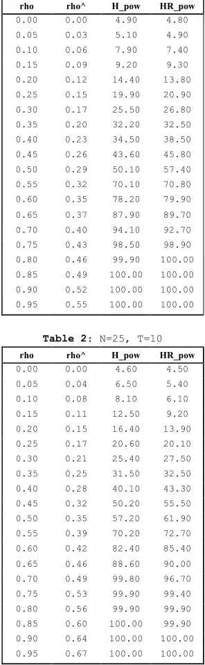
Figure 2: ‘size’ vs K

being 1/(1₋k∗), with one of [1 + 3k∗/(1₋k∗)]. It also follows that a lower bound to the distortion is provided by multiplying aχ2(k)by 1/(1−k∗).

A number of qualifications are in order. This only occurs if the inconsistency of within and between estimators is equal, and, further, the within group sum of squares matrix, and between group sum of squares matrix, are equal:

ΣZM Z,= lim N→∞

1

N N X

i=1

ZiM+Zi,=ΣQ,=

1

T ₋1Nlim→∞

1

N N X

i=1

ZiQ+Zi.

The equality of plim(bβ_{BG −}β) and plim(bβ_{W G−}β) is required to ensure that the asymptotic ‘size’ is not1. (Thus the Hausman test can be regarded as a (consistent) test of equality of these ‘inconsistencies’).The equality of ΣZM Z and ΣQ simplifies

the result and is an aid to interpretability. We also assume that the rows of Mi,

the measurement errors, are N ID(0,ΣM). Some assumption about fourth moments

is required, and this appears the simplest.

We can plot the size distortion for assumed values ofT, K,γ0_γ,γ0_[Σ

Z∗M Z∗+I]−1γ,σ2_η

andσ2_{.IfT = 5or10,1}

≤K _≤10,γ0_{γ = 1,σ}2

η =σ2 = 0.1,andγ0[ΣZ∗M Z∗+I]−1γ =

0.5, we have Figure 2, evaluated by Monte Carlo (1 million replications).

We can relax the assumtion that ΣQ=ΣZM Z by observing that V is of the form

andA is of the form

A= (k3B+k4C)−1

where

B = [ΣQ+ΣM]−1, C = [ΣZM Z+ΣM]−1

k1 = [1/(T −1)]σ∗2, k2 =σ∗∗2

d∗ = _{1 + 1/(T ₋1)_}1/2d =_{T /(T ₋1)_}1/2d,

k3 = 1/(T −1){σ∗2−c0B−1c}, <k1

k4 = {σ∗∗2−c0C−1c}, < k2

andB andC are positive definite. We see that Ais “too small”, and the test will be oversized.

V = B1/2[k1I+k2B−1/2CB−1/2+B−1/2d∗d∗0B−1/2]B1/2

A−1 = B1/2[k3I+k4B−1/2CB−1/2]B1/2

Let

D =B−1/2CB−1/2 =PΛP0

where P is orthogonal, Λ diagonal, with as diagonal elements λi the eigenvalues of D. Then

V = B1/2P[k1I+k2Λ+P0B−1/2d∗d∗0B−1/2P]P0B1/2

A = £B1/2P[k3I+k4Λ]P0B1/2

¤−1

=B−1/2P[k3I+k4Λ]−1P0B−1/2

and thus

AV = B−1/2P[k3I+k4Λ]−1[k1I+k2Λ+P0B−1/2d∗d∗0B−1/2P]P0B1/2

= B−1/2P[diag([k3+k4λi]−1){diag(k1+k2λi)

+P0B−1/2d∗d∗0B−1/2P_}]P0B1/2

which has the same eigenvalues as

{diag(k1+k2λi

k3+k4λi

)

+diag([k3+k4λi]−1{P0B−1/2d∗d∗0B−1/2P}

The second matrix has rank1, and the eigenvalues of the whole matrix are bounded between the smallest of k0,i = (k1 + k2λi)/(k3 + k4λi) and the largest of k0,i +

d∗0B−1d∗/(k3 +k4λi). λi are the eigenvalues of D = B−1/2CB−1/2, or of B−1C =

[ΣQ+ΣM][ΣZM Z+ΣM]−1. d= [ΣQ+ΣM]−1c= [ΣZMZ+ΣM]−1c=Bc=Cc

d∗0B−1d∗ = _{T /(T ₋1)_}c0Bc=_{T /(T ₋1)_}β0ΣM[ΣZM Z+ΣM]−1ΣMβ

k1 = [1/(T −1)]σ∗2,σ∗2 =σ2+β0ΣMβ =σ2+γ0γ

k2 = σ∗∗2 =σ∗2+Tσ2η

k3 = 1/(T −1){σ∗2−c0B−1c}=1/(T −1)

£

σ2+γ0γ ₋γ0[ΣZ∗_{M Z}∗+I]−1γ¤<k₁

k4 = {σ∗∗2 −c0C−1c}=σ2+γ0γ+Tσ2η−γ0[ΣZ∗M Z∗+I]−1γ < k2

Thus

σ+2 = [1/(T ₋1)]σ∗2+σ∗∗2 =k1+k2

σ++2 = [1/(T ₋1)]_{σ∗2₋c0Σ−_QM1 c_}+σ∗∗2₋c0Σ_QM−1 c=k3+k4

k0,i =

k1+k2λi

k3+k4λi

= k1+k2 +k2(λi−1)

k3+k4 +k4(λi−1)

= σ

+2_{[1 +k2(λ}

i−1)/σ+2]

σ++2_{[1 +k4(λ}

i−1)/σ++2]

=k [1 +k2(λi−1)/σ

+2_]

[1 +k4(λi−1)/σ++2]

Thus comparing this case with the B =C case, we are introducing more variability into the eigenvalues, which as we have seen , may well increase the ‘size’ of the test. (Thus the ‘size’ is sensitive to the relative magnitude of the intra-group and inter-group variations of the covariates, ΣZQZ and ΣZM Z). Our conclusion is somewhat

dispiriting: a significant Hausman statistic may arise from measurement error, as it is implicitly comparing the inconsistencies: but cannot be used to test if the inconsis-tencies are equal, as the ‘size’ may considerably exceed its nominal value, even when the inconsistenciesare equal.

6

A Power Comparison

The possible serious size distortion of the standard Hausman test motivates the for-mulation of the HR-test. Using the White estimators for the variance-covariance matrix, the test is robust to the presence of common sources of misspecification of the variance-covariance matrix, i.e. to arbitrary patterns of within groups depen-dence. In other words, using the notation in Lemma 3, AV is idempotent and the nominal size is equal to the observed one. We now use a simulation experiment to investigate the relative power of the Hausman test and the HR-test. We are inter-ested in a quantitative assessment of the possible power loss that may incur in using a robust version of the test, in absence of misspecification.

The postulated data generation process is the following. We consider the model

where y, x, uandz are(N T _×1). The null hypothesis of the Hausman test is

E(u_|x, z) = 0.

We assume z exogenous variable and we generate x correlated with u, so that the null hypothesis above is not satisfied. We consider

x=γw+ε, (39)

where x, w,ε are(N T _×1), w is an exogenous variable and(u,ε) are drawn from a bivariate normal distribution with a specified correlation structure.

The values from the exogenous regressors and the range of values for the param-eters comes from the empirical case of study analyzed in Patacchini (2002). Using UK data, the following model is estimated.

lf illvit =c+γlunf vit+πlutotit+eit, i= 1, ...,275; t= 1, ...,63

where lf illv is the logarithm of filled vacancies, lunf v is the number of unfilled vacancies (stock variable) and lutot is the number of unemployed in the area i at time t, both expressed in logs, c is a constant term, e indicates a disturbance term. The estimates of γ andπ, 0.5and 0.4, have been used in the simulation experiment for α and β respectively. Also, the best prediction for unfilled vacancies (lunf v) is found to be

lunf vit= 1.2 lnotvit, i= 1, ...,275; t= 1, ...,63,

wherelnotv is the log of the number of monthly notified vacancies (flow variable). In our experiment design, the real values forlutotandlnotvhave been used as exogenous variables, i.e. respectively z andw. The endogenous variablelunf v, i.e. x, has been constructed according to the structure (39)

x= 1.2w+ε.

The equation estimated is

y= 0.5x+ 0.4z+u,

where (u,ε) are constructed as draws from a multivariate normal distribution with the specified correlation coefficient rho of (0,0.05,0.10, . . . ,0.95).

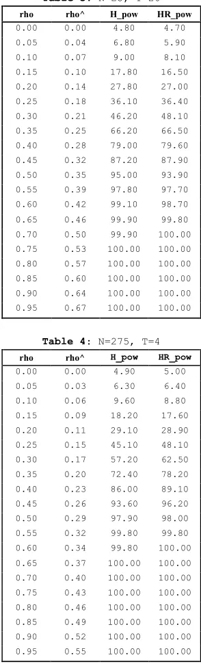
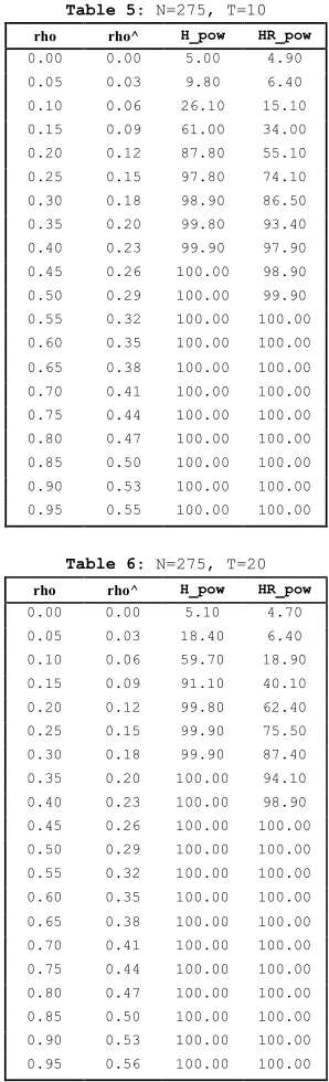
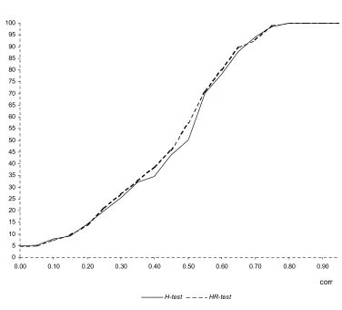
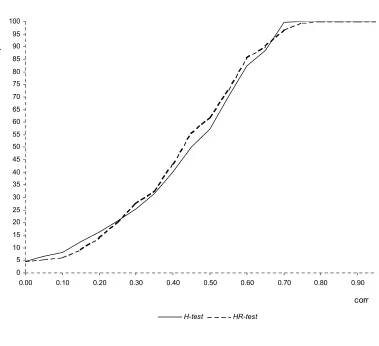
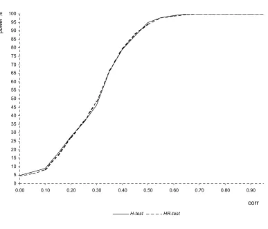
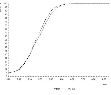
Six sample sizes, typically encountered in applied panel data studies are used. The experiment is repeated 5000 times for each sample size and level of correlation. Figures 3 to 5 contain the results of the simulation experiment. The power is expressed in percentage.

The tables displayed compare H_pow, the power of the Hausman statistic (H-test):

h=³βbwg −bβbg

´0³

b

Vwg+Vbbg

´−1³

b

Table 1: N=25, T=4

rho rho^ H_pow HR_pow 0.00 0.00 4.90 4.80 0.05 0.03 5.10 4.90 0.10 0.06 7.90 7.40 0.15 0.09 9.20 9.30 0.20 0.12 14.40 13.80 0.25 0.15 19.90 20.90 0.30 0.17 25.50 26.80 0.35 0.20 32.20 32.50 0.40 0.23 34.50 38.50 0.45 0.26 43.60 45.80 0.50 0.29 50.10 57.40 0.55 0.32 70.10 70.80 0.60 0.35 78.20 79.90 0.65 0.37 87.90 89.70 0.70 0.40 94.10 92.70 0.75 0.43 98.50 98.90

0.80 0.46 99.90 100.00

0.85 0.49 100.00 100.00

0.90 0.52 100.00 100.00

[image:28.595.211.359.121.599.2]

0.95 0.55 100.00 100.00

Table 2: N=25, T=10

rho rho^ H_pow HR_pow 0.00 0.00 4.60 4.50 0.05 0.04 6.50 5.40 0.10 0.08 8.10 6.10 0.15 0.11 12.50 9.20 0.20 0.15 16.40 13.90 0.25 0.17 20.60 20.10 0.30 0.21 25.40 27.50 0.35 0.25 31.50 32.50 0.40 0.28 40.10 43.30 0.45 0.32 50.20 55.50 0.50 0.35 57.20 61.90 0.55 0.39 70.20 72.70 0.60 0.42 82.40 85.40 0.65 0.46 88.60 90.00 0.70 0.49 99.80 96.70 0.75 0.53 99.90 99.40 0.80 0.56 99.90 99.90

0.85 0.60 100.00 99.90

0.90 0.64 100.00 100.00

0.95 0.67 100.00 100.00

[image:29.595.211.358.115.600.2]

Table 3: N=25, T=20

rho rho^ H_pow HR_pow 0.00 0.00 4.80 4.70 0.05 0.04 6.80 5.90 0.10 0.07 9.00 8.10 0.15 0.10 17.80 16.50 0.20 0.14 27.80 27.00 0.25 0.18 36.10 36.40 0.30 0.21 46.20 48.10 0.35 0.25 66.20 66.50 0.40 0.28 79.00 79.60 0.45 0.32 87.20 87.90 0.50 0.35 95.00 93.90 0.55 0.39 97.80 97.70 0.60 0.42 99.10 98.70 0.65 0.46 99.90 99.80

0.70 0.50 99.90 100.00

0.75 0.53 100.00 100.00

0.80 0.57 100.00 100.00

0.85 0.60 100.00 100.00

0.90 0.64 100.00 100.00

0.95 0.67 100.00 100.00

Table 4: N=275, T=4

rho rho^ H_pow HR_pow 0.00 0.00 4.90 5.00 0.05 0.03 6.30 6.40 0.10 0.06 9.60 8.80 0.15 0.09 18.20 17.60 0.20 0.11 29.10 28.90 0.25 0.15 45.10 48.10 0.30 0.17 57.20 62.50 0.35 0.20 72.40 78.20 0.40 0.23 86.00 89.10 0.45 0.26 93.60 96.20 0.50 0.29 97.90 98.00 0.55 0.32 99.80 99.80

0.60 0.34 99.80 100.00

0.65 0.37 100.00 100.00

0.70 0.40 100.00 100.00

0.75 0.43 100.00 100.00

0.80 0.46 100.00 100.00

0.85 0.49 100.00 100.00

0.90 0.52 100.00 100.00

0.95 0.55 100.00 100.00

[image:30.595.210.359.109.599.2]

Table 5: N=275, T=10

rho rho^ H_pow HR_pow 0.00 0.00 5.00 4.90 0.05 0.03 9.80 6.40 0.10 0.06 26.10 15.10 0.15 0.09 61.00 34.00 0.20 0.12 87.80 55.10 0.25 0.15 97.80 74.10 0.30 0.18 98.90 86.50 0.35 0.20 99.80 93.40 0.40 0.23 99.90 97.90

0.45 0.26 100.00 98.90

0.50 0.29 100.00 99.90

0.55 0.32 100.00 100.00

0.60 0.35 100.00 100.00

0.65 0.38 100.00 100.00

0.70 0.41 100.00 100.00

0.75 0.44 100.00 100.00

0.80 0.47 100.00 100.00

0.85 0.50 100.00 100.00

0.90 0.53 100.00 100.00

[image:30.595.211.358.354.597.2]

0.95 0.55 100.00 100.00

Table 6: N=275, T=20

rho rho^ H_pow HR_pow 0.00 0.00 5.10 4.70 0.05 0.03 18.40 6.40 0.10 0.06 59.70 18.90 0.15 0.09 91.10 40.10 0.20 0.12 99.80 62.40 0.25 0.15 99.90 75.50 0.30 0.18 99.90 87.40

0.35 0.20 100.00 94.10

0.40 0.23 100.00 98.90

0.45 0.26 100.00 100.00

0.50 0.29 100.00 100.00

0.55 0.32 100.00 100.00

0.60 0.35 100.00 100.00

0.65 0.38 100.00 100.00

0.70 0.41 100.00 100.00

0.75 0.44 100.00 100.00

0.80 0.47 100.00 100.00

0.85 0.50 100.00 100.00

0.90 0.53 100.00 100.00

0.95 0.56 100.00 100.00

with HR_pow, the power of the robust Hausman statistic (HR-test) obtained using the auxiliary regression detailed in Section (3):

hr =³βb_wg−bβ_bg´0

·

\

V ar³βb_{wg −}bβ_bg´¸

−1³

b

β_{wg −}βb_bg´,

with different sample sizes. Figures 6 to 11 contained in Appendix 6 illustrate the relative power functions. The significance level has been fixed at 5%. rhoˆ is the estimated level of correlation between x and u conditioned upon w. For each level

of rho, H_pow and HR_pow indicate the percentage of times we reject a false

hypothesis if we use respectively the H-test or the HR-test.

In Table 1, 2 and 3 the number of cross-sectional units is held fixed at 25 and the number of time periods is varied respectively between 4, 10 and 20. In Table 4, 5 and 6 the number of cross-sectional units is held fixed at 275 and the number of time periods is varied respectively between 4,10 and 20. Table1 to 4 show that the performance of the HR-test is comparable with the one of the H-test, even better for values ofrho greater than 0.3. In larger samples (Table 5 and 6) the performance of theH-test is superior but the power loss of the HR-test is not serious. The HR-test gives a very high rejection frequency for the false hypothesis of absence of correlation between x and u, starting from levels of correlation around 0.3 (86.5% and 87.4% respectively in Table 5 and 6) and it detects the endogeneity problem almost surely as soon as rho is higher than 0,4 (97.9% and98.9% respectively in Table 5 and 6). Taking the results as a whole, the simulation experiment provides evidence that the performance of theHR-test in terms of power is satisfying in large samples and even better than the one given by the H-test in small samples.

In addition, it is worthwhile noting that a version of the Hausman test imple-mented in most econometric software, which is generally used in empirical studies, is the one based on the comparison betweenβb_wg and bβ_BN, i.e.

h=³bβ_wg−βb_BN´

0³

b

Vwg−Vbbg

´−1³

b

β_wg−bβ_BN´.

The problem related with this approach is that, in finite samples, the difference between the two estimated variance-covariance matrices of the parameters estimates (i.e. Vbwg −Vbbg) may not be positive definite. In this cases, the use of a code

imple-menting a different Hausman statistic or the formulation of the Hausman test using an auxiliary regressions (e.g. the one proposed by Davidson and McKinnon (1993, p. 236), which is now already implemented in some statistical packages, or the (robust) one presented in this paper) are the only possibilities to get a test outcome.

7

Conclusions

and empirical.

From a theoretical point of view, it is shown that the assumptions in Lemma 2.1. in Hausman (1978) are sufficient but not necessary. The main result is that the attainment of the absolute Fisher lower bound can be replaced by the attainment of a relative minimum variance bound.

From an empirical point of view, the main implication of this paper is a caveat on the use of the standard Hausman test framework for correlated effects in applied panel data studies. Our claim is that the application of this test is often not correct from a methodological point of view. The assumptions underlying the construction of the Hausman statistic (Hausman,1978) may be rarely satisfied in empirical work. An analytical investigation of the size of the test shows that, at least in some cases, the distortion is substantial. The econometrics of panel data offers a variety of estimators for the same parameters. Our recommendation is to use the Hausman test framework for the comparison of appropriate panel data estimators, but to construct a version of the test robust to deviations from the classical errors assumption. This test, the HR-test, gives correct significance levels in common cases of misspecification of the variance-covariance matrix and has a power comparable to the Hausman test when no evidence of misspecification is present. The power of theHR-test is even higher in small samples. It can be easily implemented using a standard econometric package.

References

[1] Arellano, M. (1993). On the Testing of Correlated Effects with Panel Data, Journal of Econometrics, 59, 87-97.

[2] Ahn, S.C. and Low, S. (1996). A Reformulation of the Hausman Test for Regres-sion Models with Pooled Cross Sectional Time Series Data, Journal of Econo-metrics, 71, 309-319.

[3] Balestra, P. and Nerlove, M. (1966). Pooling Cross Section and Time Series Data, Econometrica, 34, 585-612.

[4] Baltagi, B.H. (1996). Testing for Random Individual and Time Effects using a Gauss-Newton Regression, Economics Letters, 50, 189-192.

[5] Baltagi, B.H. (1997). Problems and Solutions,Econometric Theory, 13, 757.

[6] Baltagi, B.H. (1998). Problems and Solutions,Econometric Theory, 14, 527.

[7] Davidson, R. and MacKinnon, J.G. (1993). Estimation and Inference in Econo-metrics, Oxford University Press.

[9] Golub, G.H. and Van Loan, C.F. (1983). Matrix Computations, third edition, North Oxford Academic Press.

[10] Griliches, Z. and Hausman, J.A. (1986). Error in Variables in Panel Data,Journal of Econometrics, 31, 93-118.

[11] Hansen, L. (1982). Large Sample Properties of Generalized Method of Moment Estimators, Econometrica, 50, 517-533.

[12] Hausman, J.A. (1978). Specification Tests in Econometrics, Econometrica, 46, 1251-1271.

[13] Hausman, J.A. and Taylor, W.E. (1981). Panel Data and Unobservable Individ-ual Effects, Econometrica, 49, 1377-1398.

[14] Holly, A. (1982). A Remark on Hausman’s Specification Test,Econometrica, 50, 749-760.

[15] Kakwani, N.C. (1967). The Unbiasedness of Zellner’s Seemingly Unrelated Re-gression Equation Estimators, Journal of the American Statistical Association, 82, 141-2

[16] Maddala, G.S. (1971). The Use of Variance Components Models in Pooling Cross Section and Time Series Data, Econometrica, 39, 341-358.

[17] Magnus, J.R. and H. Neudecker, (1988)Matrix Differential Calculus John Wiley and Sons.

[18] Muirhead, R.J. (1982). Aspects of Multivariate Statistical Theory, New York: John Wiley and Sons.

[19] Nerlove, M. (1971). A Note on Error Components Models, Econometrica, 39, 383-396.

[20] Patacchini, E. (2002). Unobservable Factors and Panel Data Sets: the Case of Matched Employee-Employer Data, Discussion Papers in Economics and Econo-metrics n.0202, University of Southampton.

[21] Johnson, N.L. and Kotz, S. (1970). Continuous Univariate Distributions, New York: John Wiley and Sons.

[22] Vuong, Q. (1989). Likelihood Ratio Tests for Model Selection and Non-Nested Hypotheses, Econometrica, 57, 307-333.

[23] White, H. (1984). Asymptotic Theory for Econometricians, Academic Press, New York.

8

Appendix 1

Lemma 4 If t1 andt2 are unbiased estimators ofθ ∈Rp,with t1 minimum variance (MV) at least in the set

T =_{t:t=At1+ (I−A)t2}

then

Cov(t1, t−t1) =0

where Iis the identity matrix, 0 a null matrix, and A_∈Rp×p is fixed.

Proof.

t=At1+ (I−A)t2 =t1+ (I−A)(t2−t1)

=t1 +Bd, say, B∈Rp×p

V ar(t) =E_{[t1−θ+Bd] [t1−θ+Bd]0}

=V ar(t1) +Cov(t1, d)B0+BCov(d, t1) +BV ar(d)B0.

Thus we can write

V ar(t)₋V ar(t1) =CB0+BC0+BDB0.

The minimum variance property oft1 implies this difference is positive semi-definite, and thus for every λ_∈Rp_{,and B}

∈Rp×p_,

Q=λ0(CB0+BC0+BDB0)λ _≥0.

However, for the particular case of

B=₋CD−1

Q=λ0(₋CD−1C0₋CD−1C0+CD−1DD−1C0)λ

=λ0(₋CD−1C0)λ

which satisfies the required inequality if and only if

C=0.

Further, for anyB _∈Rp×p

t₋t1 =Bd,

Remark 5 We exclude the case where D is singular, as in that case replacing D−1 with a pseudo-inverse D+ _{such that D}+_DD+_=D+ _{reveals that all that is required is} CD+C0 _{=0, or that Chas rows orthogonal to the eigenvectors of Dcorresponding to}

the non-zero roots. As an example, consider the case where some elements of t1 and

t2 coincide. It is simplest to exclude the coincident elements, and apply the argument above to the reduced vectors so formed.

Remark 6 This lemma implies that the MV unbiased estimator is uncorrelated with its difference from any other unbiased estimator, and the MV linear unbiased estima-tor is uncorrelated similarly.

We next show that a set of the form_T in Lemma1contains a minimum variance estimator. First, it is convenient to re-write the basis of the set in terms oft1 andt3, where Cov(t3, t1) =0.

Lemma 7 If t1 and t2 are unbiased estimators of θ ∈ Rp with covariance matrix

·

V11 V12 V21 V22

¸

, the set

T =_{t:t=At1+ (I−A)t2} can also be defined in terms of t1 and

t3 =Bt1+ (I−B)t2

where

Cov(t3, t1) =0

as

T =_{t:t=Ct1+ (I−C)t3} with

B =₋V21(V₁₁₋V21)−1,I₋B =V11(V₁₁₋V21)−1

V ar(t3) =₋DV−₁₁1D0+DV₂₁−1V22V12−1D0,D =

£

V−₂₁1₋V₁₁−1¤−1

C=A(V₁₁₋V21) +V₂₁)V−₁₁1,I₋C= (I₋A)(V₁₁₋V12)V−₁₁1

V ar(t) =CV11C0+ (I−C)V ar(t3)(I−C)0

Proof.

Cov(t3, t1) =E{[Bt1+ (I−B)t2−θ][t1−θ]0}

Now

£

V11(V₁₁₋V21)−1V21

¤−1

=V−₂₁1(V₁₁₋V21)V−₁₁1 =V−₂₁1₋V₁₁−1

and

£

V21(V₁₁₋V21)−1V11

¤−1

=V−₁₁1(V₁₁₋V21)V−₂₁1 =V−₂₁1₋V₁₁−1.

It follows that

V11(V₁₁₋V21)−1V21 =V21(V11−V21)

−1

V11 (1.1)

and thus

Cov(t3, t1) =0

To findV ar(t3), as

t3 =Bt1+ (I−B)t2

V ar(t3) =BV11B0+(I−B)V₂₁B0+BV12(I−B)0+(I−B)V₂₂(I−B)0

BV11B0 =V21(V11−V21)

−1

V11(V11−V21)− 10_V0

21

(I₋B)V₂₁B0 =₋V11(V₁₁₋V21)−1V21(V11−V21)− 10_V0

21 Identity (40) implies equality between these expressions.

BV12(I₋B)0 =₋V21(V₁₁₋V21)−1V12(V₁₁₋V21)−10V0₁₁

Transposing (40), this becomes the same as the expression for BV11B0.

(I₋B)V₂₂(I₋B)0 =V11(V₁₁₋V21)−1V22(V₁₁₋V21)−10V₁₁0

This suggests writing the matrix in (40) as

D=£V₂₁−1₋V−₁₁1¤−1

to give

V ar(t3) =₋DV−₁₁1D0+DV−₂₁1V22(V021)

−1 D0

Remark 8 Again, we are assuming non-singularity, in particular of V21. One could apply the steps above to zero a single non-zero element of V21, by shrinking t1 and

t2 to the corresponding elements. Repeated application would then replace V21 with a null matrix.

Lemma 9 If t1 and t2 and T are as in Lemma (2) but withV12=0 then t has the minimum variance in _T if

A= [V−₁₁1+V₂₂−1]−1V−₁₁1

Proof. Let this value of t be tM, the corresponding A be AM, and VM =

V ar(tM). Let

AM=EV−111,⇒I−AM=EV−221

We have

V ar(tM) =EV−111V11V−111E+EV−

1

22V22V−221E =E£V₁₁−1+V−₂₂1¤E =E.

Moreover,

Cov(tM, t1 −t2) =Cov(AMt1+ (I−AM)t2, t1 −t2)

=E[_{EV−₁₁1(t1 −θ) +EV22−1(t2−θ)}{t01−t02}] =E[E(V−₁₁1V11−V22−1V22)] = 0.

If t _∈T,

t=At1+ (I−A)t2

= (AM +A−AM)t1+ (I−AM −A+AM)t2 =tM + (A−AM)(t1−t2)

Thus

V ar(t) =V ar(tM) + (A−AM)V ar(t1−t2)(A−AM)0

and thusV ar(t) exceeds V ar(tM) by a positive semi-definite difference, and thustM

is the minimum variance estimator in _T.

Finally, we establish the large sample equivalent of Lemma 1.

Lemma 10 Consider t0_∗ = [t01, t20],θ0_∗ = [θ0,θ0]

√

n(t_∗−θ_∗)_−→D (0,

·

V11 V12 V21 V22

¸

)

where V11 is the ‘asymptotic variance’, Avar, of t1 and V12 is the ‘asymptotic co-variance’ of t1 and t2,Acov(t1, t2). If t1 is asymptotically minimum variance at least in the class

T =_{t:t=At1+ (I−A)t2},A∈Rp×p, fixed, then if t0

d = [t01,[t−t1]0],θ0d = [θ0,00]

√

n(td−θd)

D −→(0,

·

V11 0

0 V ar(t)₋V11

¸