A Fully Unsupervised Texture Segmentation Algorithm

A Fully Unsupervised Texture Segmentation

Algorithm

Mohammad F. A. Fauzi and Paul H. Lewis

Department of Electronics and Computer Science

University of Southampton

Southampton, SO17 1BJ, UK

{

mfaf00r,phl

}

@ecs.soton.ac.uk

Abstract

This paper presents a fully unsupervised texture segmentation algorithm by using a modified discrete wavelet frames decomposition and a mean shift algorithm. By fully unsupervised, we mean the algorithm does not require any knowledge of the type of texture present nor the number of textures in the image to be segmented. The basic idea of the proposed method is to use the modified discrete wavelet frames to extract useful information from the image. Then, starting from the lowest level, the mean shift algorithm is used together with the fuzzy c-means clustering to divide the data into an appropriate number of clusters. The data clustering process is then refined at every level by taking into account the data at that particular level. The final crispy segmentation is obtained at the root level. This approach is applied to segment a variety of composite texture images into homogeneous texture areas and very good segmentation results are reported.

1

Introduction

Texture analysis is not a new topic in the vision community, as it has been investigated in its own right for the last thirty years by researchers in psychophysics and more recently computer vision. In the field of computer vision, texture plays an important role in low level image analysis and understanding. Its potential application range has been shown in various areas such as analysis of remote sensing images, industrial monitoring of product quality, medical imaging, and recently, content-based image and video retrieval. There is no formal or unique definition of texture, making texture analysis a difficult and challeng-ing problem.

It is therefore inefficient to expect the number of textures to be manually provided for all the images. An automatic texture detection and segmentation algorithm, which we termed fully unsupervised segmentation, is therefore needed to suit this kind of application.

In this paper, a novel texture segmentation method that is fully unsupervised (i.e. without any a priori knowledge on either the type of textures or the number of textures in the image) is presented. The method uses a modified discrete wavelet frames (DWF) decomposition to extract important features from an image before a mean shift algorithm is used together with a fuzzy c-means (FCM) clustering to cluster or segment the image into different texture regions. The proposed algorithm has the advantage of high accuracy while maintaining low computational load. We will also show the advantage of using the modified DWF over the standard DWF and the wavelet transform, and demonstrate how using the mean shift together with the FCM helps in speeding up the fuzzy clustering process. The rest of the paper is organized as follows: in the next section, related work concerning texture segmentation is briefly reviewed. This is followed by a brief review of the discrete wavelet frames in section 3. In section 4 we explain the algorithm for the mean shift. The implementation of the segmentation method is presented in section 5. In section 6 results obtained using our technique on a variety of image data are presented. We conclude the paper in section 7.

2

Related Works

There are already a large number of texture segmentation algorithms in the literature. Texture segmentation usually involves the combination of texture feature extraction tech-niques with a suitable segmentation algorithm. Among the most popular feature extrac-tion techniques used for texture segmentaextrac-tion are the Gabor filters, Markov random fields, Laws’ texture features and wavelets, while split-and-merge, region growing and cluster-ing are the most commonly used segmentation algorithms. Due to its multiresolution property, wavelets have provided a new dimension to the field of computer vision, and many studies have been conducted utilizing wavelets in texture segmentation. Promising results have been reported in [5, 14, 16], among others.

IMAGE

(a)

LL2

HH2 HL2

LH2

LH1

HH1 HL1

(b)

2nd level coefficients

1st level coefficients

(c)

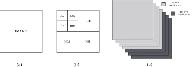
Figure 1: (a) An image and its, (b) wavelet transform, (c) discrete wavelet frames

3

Discrete Wavelet Frames

The wavelet transform [12] analyses a signal based on its content in different frequency ranges. Therefore it is very useful in analysing repetitive patterns such as texture. The transform uses a family of wavelet functions and its associated scaling function to decom-pose the original image into different channels, namely thelow-low,low-high,high-low

andhigh-high(LL,LH,HL,HHrespectively) channels. The decomposition process can be recursively applied to the low frequency channel (LL) to generate decomposition at the next level. Thequadrature mirror filtersare used to implement the wavelet transform by low- and high-pass filtering the original image followed by a sub-sampling process, resulting in an output with the same size as the input. Figure 1(b) shows a 2-level wavelet transform decomposition of an image.

Discrete wavelet frames (DWF) [16], or an over-complete wavelet transform, is nearly identical to the standard wavelet transform, except that one up-samples the filters, rather than down-samples the image. While the frame representation is over-complete, and computationally more intensive than the wavelet transform, it holds the advantage of be-ing translationally invariant. Given an image, the DWF decomposes it usbe-ing the same method as the wavelet transform, but without the sub-sampling process. This results in four filtered images with the same size as the input image. The decomposition is then continued in theLLchannels only as in the wavelet transform, but since the image is not sub-sampled, the filter has to be up-sampled by inserting zeros in between its coef-ficients. Figure 1 (b) and (c) shows the difference between the discrete wavelet frames decomposition and the standard wavelet transform.

4

Mean Shift Algorithm

x x x x x _{x x}

x x

x x x x x x x_{x x} x

O O

Data point Convergence

point

x x x x x xx x x

xx x

x x x x x x x

O

O

Data point

Convergence point

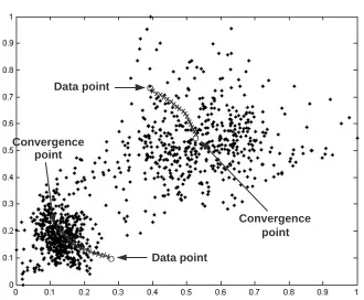
Figure 2: Mean shift convergence of data points

readers are referred to Comaniciu and Meer [7].

However, Comaniciu and Meer used a simple nearest neighbour clustering to associate each data point to its cluster centre for their colour features. We find this approach is too basic to be used for texture features, since unlike colour, the distribution of texture feature data in the feature space is more complex and therefore needs a more robust clustering technique. Furthermore, since our method uses a multiresolution feature extraction in discrete wavelet frames, the decision about cluster membership for a pixel only needs to be decided at the root level. The clustering output at all levels, except the root, only serve as intermediate results, and therefore is better represented by some sort of a membership function instead of a membership class. For these reasons, we opt to use the fuzzy c-means clustering to cluster the data, while the mean shift algorithm is just used to estimate the number of clusters and the cluster centres.

5

Texture Segmentation

The texture segmentation problem deals with composite textures, i.e. an image contains several different types of texture. Our proposed texture segmentation algorithm has a hier-archical structure and consists of two phases: a top-down decomposition phase followed by a bottom-up segmentation phase.

5.1

Top-Down Decomposition Phase

In the top-down decomposition phase, we perform aK-level discrete wavelet frames de-composition. For a 2n×2nimage, this results in 3K+1 planes of 2n×2ndata, which is a large amount of data for use with the mean shift algorithm. For the algorithm to be efficient computationally, it is necessary to find a way to reduce the amount of data to be clustered. Recall that for the standard wavelet transform, the output of the filter is sub-sampled at each level resulting in an output with the same size as the input image, while discrete wavelet frames are an over-complete wavelet transform where all the output data are preserved. If we sample the DWF output every 2k_{samples, wherek=1,...,Kis the}

(a) (b)

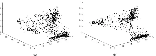
Figure 3: 3D plot in the feature space for (a) wavelet transform coefficient, (b) modified DWF coefficient

However, we do not want to use the wavelet transform coefficients for segmentation as they are of a very high variance. For example, the 3rd level coefficients of the wavelet transform are sampled every 8 coefficients both horizontally and vertically, and if we plot these into a feature space, there will not be well defined clusters due to the high variance, even after applying some smoothing process. While the wavelet transform is perfectly reconstructable, thus making it very good in some other fields, it is not very suitable for image segmentation, at least for the fully unsupervised case. If the coefficients of the discrete wavelet frames are carefully chosen rather than simply throwing away every other data point as in the wavelet transform, well defined clusters can be obtained and the amount of data can also be reduced greatly.

A simple yet reliable method is to take the mean of energy within a distinct blocks. For each filtered image, the DWF coefficients are divided into distinct blocks of size 2k×2k, and the mean absolute value of the data within the blocks are taken as the new coefficients of the DWF at that level. This results in data reduction of factor (2k×2k) for that particular filtered image. If this procedure is repeated for every filtered image of the DWF we will have the same output configuration as the wavelet transform but with better coefficients. Figure 3 shows a 3D plot of coefficients at level 3 for both the wavelet transform and the modified DWF of the same image consisting of 3 textures. Notice the data of the wavelet transform coefficients are poorly scattered and end up detecting 4 clusters instead of 3.

At this point, we label the original image of size 2n_×2n_{with level index 0 (the root}

level), the four sub-images of size 2n−1_×2n−1_{with level index 1 and so on. Since the}

discrete wavelet frames provide good spatial and frequency energy localization, we may take the energy value of each modified DWF coefficient as an energy feature. However, the variance of the feature is still high since only one sample is used. By assuming that neighbouring DWF coefficients are identically and independently distributed, the variance can be reduced by performing a local averaging or smoothing operation. On the one hand, it is desirable to have a large window to reduce the statistical variations. On the other hand, since a large window centred at points in the texture boundary region may contain multiple texture classes, the window size has to be small.

artificially dominate the clustering process.

5.2

Bottom-Up Segmentation Phase

In the bottom-up phase, we start with levelKand produce an intermediate segmentation result for levelK−1 using the four sub-images available at level K. To generate the intermediate segmentation, the four sub-images of size 2n−K×2n−K are integrated in a way that it can be viewed as four-dimensional 2n−K×2n−K data, before the mean shift algorithm is applied and provides us with the number of clusters detected in the data as well as the cluster centre positions. As mentioned in the last section, the fuzzy c-means clustering (FCM) is chosen above other clustering techniques and is applied to the four-dimensional data using the information provided by the mean shift. The fuzzy c-means clustering algorithm is an iterative procedure described in the following:

Fuzzy C-Means Clustering Algorithm

GivenMinput data{xm;m=1,...,M}, the number of clustersC(2≤C<M), and the fuzzy weighting exponent w, 1<w<∞, initialize the fuzzy membership functionsu(c,0m) withc=1,...,Candm=1,...,Mwhich are the

entry of aC×MmatrixU(0)_{. Perform the following for iterationl=1,2,...:}

1. Calculate the fuzzy cluster centresvclwithvc=∑Mm=1(uc,m)wxm/∑Mm=1(uc,m)w

2. UpdateU(l)withuc,m=1/∑Ci=1

_d

c,m

di,m

2

w−1

where(di,m)2=xm−vi2and · is any inner product

induced norm.

3. CompareU(l)_withU(l+1)_{in a convenient matrix norm. IfU}(l+1)_−U(l) _{≤εstop; otherwise return to}

step 1.

The value of the weighting exponent,wdetermines the fuzzyness of the clustering de-cision. A smaller value ofw, i.e.wis close to unity, will give the zero/one hard decision membership function, and a largerwcorresponds to a fuzzier output. Our experimen-tal results suggest thatw=2 is a good choice. The advantage of using the mean shift algorithm together with the fuzzy c-means clustering is demonstrated here. The fuzzy c-means algorithm is not a fully unsupervised clustering method as it requires the number of clusters to be known a priori. Besides that, one other drawback of the fuzzy c-means is finding the best way to initialize the fuzzy membership function.

The FCM algorithm finds a local minimum ofΣC_c=1ΣM_m=1u_cw_,md_c2_,mby solvinguc,mand

vc, and its output depends on the initial value ofU(0). Various methods have been

pro-posed on the best way to initializeU(0)such as the maximin distance algorithm. But by using the mean shift, it not only provides the FCM with the number of clusters, but also the cluster centres, meaning that the initial value ofU(0)is already quite close to the final value ofU(0). Hence part of the task of the FCM, that is to find appropriate cluster cen-tres, is done. Experiments have shown that the FCM algorithm terminates after just a few iterations, thanks to the precise location of the cluster centres.

The output of the fuzzy c-means is a 2n−K_×2n−K _{membership function of N}

c

di-mension, whereNcis the number of clusters. Each element of the membership function

describes the membership value with respect to a particular type of cluster and the sum of these elements is equal to 1. The membership function is then interpolated to size 2n−K+1×2n−K+1so that it has the same size with the data at the following level. For sim-plicity, a linear interpolation algorithm is used to interpolate the membership function.

shift and FCM processes. These procedures of data integration, mean shift, clustering and interpolation are applied recursively from bottom to top so that we eventually obtain the segmentation result of the root level, i.e. the original image. The final crispy segmentation at level 0 can be determined by assigning each pixel to the class where it has the highest probability of membership. Note that the number of clusters detected by the mean shift algorithm can be different at each level. We might get a wrong number of clusters in the bottom level, but that is just an intermediate result, where not all data are utilized. What matters is the final segmentation result, after all data is taken into account. The incorrect number of clusters in the bottom level might be refined by the data at the higher levels.

6

Experimental Results

We applied our texture segmentation algorithm to several images of composite textures with size 256×256 pixels and 256 grey levels. Textures from the Brodatz album [1] are used to made up the composite texture images. None of the textures used in our experiment can be discriminated by grey level values alone. An image is decomposed using the modified DWF for up to three levels using, in our case, an 8-tapDaubechies

wavelet filter. The radius,hfor the mean shift algorithm is critical, and from experiment a suitable value ofhat all levels is found to be 0.2.

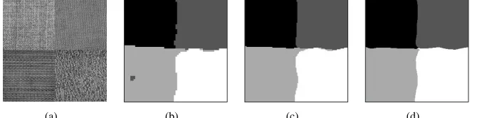
Figure 4 shows the sequence of segmentation results obtained at each level for a com-posite texture image which consists of 4 textures from the Brodatz album, D017, D024, D055 and D077. In this example, the initial segmentation result obtained at level 2 already gives a quite good segmentation and is used as a basis for higher level processing. It can be clearly seen that the coefficients from the higher levels help in refining the boundary of the textures.

(a) (b) (c) (d)

Figure 4: (a) 4-textured image, and its segmentation result at, (b) level 2 (64×64), (c) level 1

(128×128), (d) level 0 (256×256, final result)

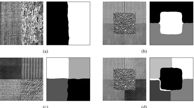
Figure 5 shows an example of applying the texture segmentation algorithm to a num-ber of images with different numnum-ber of textures. The 2-textured image consists of texture D012 and D017, the 3-textured image of texture D054, D074 and D102, the 4-textured image of texture D001,D011,D018 and D026, while the 5-textured images consists of texture D001, D053, D065, D074 and D102. All the results in Figure 5 show a correctly identified number of texture as well as good segmentation. All together, we have applied our algorithm to 50 composite textures, and the results are summarized in Table 1.

(a) (b)

(c) (d)

Figure 5: Segmentation result for different number of textures

and D102. From the figure, it is clear that the incorrect segmentation is caused by the fact that the top half texture appears to contain two visually different regions. For the 5 incorrect cases, the cause is either the same problem as above, or the fact that two textures are almost visually the same.

Number of Number of Images with Number of textures detected textures images tested correctly detected for the wrong detection case

in an image number of textures 2 3 4 5

2 16 15 1

3 12 11 1

4 13 12 1

5 9 7 2

Total 50 45 (90%) 1 2 2

Table 1: Percentage of correctly detected number of textures.

Table 2 shows the percentage of segmentation errors for the five correctly segmented textures shown in Figure 4 and 5. All of the images give an error percentage of below 5% which is a good result. Notice that the more texture boundaries there are, the more difficult decisions must be made, resulting in an increasing number of misclassified pixels. Non-boundary pixels seem to be well distinguished by the proposed algorithm. All together from the 45 correctly segmented images, we obtain an average of just 3.72% misclassified pixels.

Figure 7 shows segmentation results for synthetic textures composed of the +- and L-symbols. This texture pair has a spectrum with the same magnitude but different phases. Since the illumination of both textures are the same, this example also shows that it is the surface texture, not the illumination conditions that is being classified. Figure 8 shows a segmentation result on a real scene image, where the algorithm correctly segmented the sky, mountain and water into 3 separate regions. Since it is difficult to define an objective boundary for these examples, the percentage of segmentation errors cannot be measured. However, from the figures, it is clear that the proposed algorithm works well in distinguishing synthetic texture as well as real scene image.

Image Textures Misclassified Percentage pixels of error

Figure 4 4 1654 2.52% Figure 5(a) 2 621 0.90% Figure 5(b) 3 1771 2.70% Figure 5(c) 4 1615 2.46% Figure 5(d) 5 2816 4.29%

Table 2: Percentage of misclassified pixels

based on the wavelet transform segmentation, i.e. the data to be clustered by the mean shift and the FCM is generated by the wavelet transform instead of the modified DWF. Figure 9 compares the performance of the modified DWF with the wavelet transform method for the image in Figure 5(d). Clearly, the wavelet transform fails to provide good clusters in the feature space resulting in a poor segmentation. Also, the sampling of poorly scattered data points during the mean shift results in a rather inconsistent segmentation for the wavelet transform-based segmentation. The modified DWF is therefore superior to the wavelet transform in terms of segmentation performance, and is superior to the standard DWF in terms of computational speed.

Figure 6: Example of incorrect segmenta-tion

Figure 7: Segmentation result of synthetic textures

Figure 8: Segmentation result of real image texture

Figure 9: Result using modified DWF (left) and wavelet transform (right)

7

Conclusion

tex-tures, synthetic textures and real scene images, while maintaining the low computational load.

References

[1] P. Brodatz. Textures: A Photographic Album for Artists & Designers. Dover Publications,

Inc., New York, 1966.

[2] J.M.H. Du Buf, M. Kardan, and M. Spann. Texture feature performance for image

segmenta-tion.Pattern recognition, 23(3/4):291–309, 1990.

[3] K. I. Chang, Kevin W. Bowyer, and Munish Sivagurunath. Evaluation of texture segmentation

algorithms. InIEEE Conference on Computer Vision and Pattern Recognition, pages 294–299,

1999.

[4] Tian-Horng Chang, Yu-Chuan Lin, and C. C. Jay Kuo.Techniques In Texture Analysis.

Med-ical Imaging Systems Techniques and Applications: Computational Techniques, Edited by C. T. Leondes. Gordon and Breach Science Publishers, 1998.

[5] Tianhorng Chang and C. C. Jay Kuo. Texture segmentation with tree-structured wavelet

trans-form. InProceedings of the IEEE-SP International Symposium on Tine-Frequency and

Time-Scale Analysis, pages 543–546, 1992.

[6] Yizong Cheng. Mean shift, mode seeking, and clustering. IEEE Transactions on Pattern

Analysis and Machine Intelligence, 17(8):790–799, 1995.

[7] Dorin Comaniciu and Peter Meer. Mean shift: A robust approach toward feature space analy-sis.IEEE Transactions on Pattern Analysis and Machine Intelligence, 24:603–619, 2002.

[8] K. Fukunaga and L. D. Hostetler. The estimation of the gradient of a density function, with

applications in pattern recognition. IEEE Transactions on Information Theory, IT-21(1):32–

40, January 1975.

[9] Joseph P. Havlicek and Peter C. Tay. Determination of the number of texture segments using

wavelets.Electronic Journal of Differential Equations, Conf. 2:July, 61–70 2001.

[10] Anil K. Jain and Farshid Farrokhnia. Unsupervised texture segmentation using gabor filters. Pattern Recognition, 24(12):1167–1186, 1991.

[11] Andrew Laine and Jian Fan. Texture classification by wavelet packet signatures.IEEE

Trans-actions on Pattern Analysis and Machine Intelligence, 15(11):1186–1191, November 1993.

[12] Stephane G. Mallat. A theory for multiresolution signal decomposition: The wavelet

repre-sentation.IEEE Transactions on Pattern Analysis and Machine Intelligence, 11(7):674–693,

July 1989.

[13] Nikos Paragios and Rachid Deriche. Geodasic active contours for supervised texture

segmen-tation. InIEEE Computer Society Conference on Computer Vision and Pattern Recognition,

volume 2, pages 422–427, 1999.

[14] Robert Porter and Nishan Canagarajah. A robust automatic clustering scheme for image

segmentation using wavelets. IEEE Transactions on Image Processing, 5(4):662–665, April

1996.

[15] S. N. Talbar, R. S. Holambe, and T. R. Sontakke. Supervised texture classification using

wavelet transform. InProceedings of the 4th International Conference on Signal Processing

(ICSP ’98), volume 2, pages 1177–1180, 1998.

[16] Michael Unser. Texture classification and segmentation using wavelet frames.IEEE