High Redshift LAEs and their Cosmic Evolution: Morphologies, SFR and AGN Activity from z~2 to 6

High Redshift LAEs and their Cosmic Evolution:

Morphologies, SFR and AGN Activity from z

∼

2 to 6

?

Cassandra Barlow-Hall

_†

_{, Joseph Bramwell}

_{, Daniel Hodder}

_{, Michael Merrett}

_,

Adam Russ

_{, Oliver Wareing}

_{& David Sobral}

_‡

1 _{Department of Physics, Lancaster University, Lancaster, LA1 4YB, UK}

Accepted 29 May 2019. Received 29 May 2019; in original form 25 March 2019

ABSTRACT

We studied a large sample of ∼4000 high redshift Lyman-alpha Emitters (LAEs) in order to determine their properties and infer how they might have evolved into the local Universe. This was done through the exploration of the SC4K survey (Sobral et al. 2018a) and making use of the Hubble Space Telescope (HST), Chandra X-ray Observatory (Chandra) and the Very Large Array (VLA). We find that SC4K LAEs are mostly (69±4%) compact disky galaxies (average S´ersic index, n = 1.9±2.2) The average star formation rate SFRLyαof LAEs is≈17 Myr−1. We find that SFR increases with increasing stellar mass. We also observed a characteristic ‘peak’ in SFR at M∼109.3M, at redshiftz∼2.5, and progressing to higher stellar masses at higher redshifts. We find a total of 303 X-ray or radio detected active galactic nuclei (AGN) within the SC4K catalogue. These AGN have a range of black hole accretion rates (BHARs) from ∼0.03 Myr−1 to ∼3.3 Myr−1. The AGN fraction increases with increasing Lyα luminosity and decreases with increasing redshift, peaking atz ∼ 3. LAEs found atz∼2−6 with a stellar mass M∼1010_M

and a SFR∼5.4 Myr−1are consistent with being progenitors of Milky Way-like galaxies progenitor. Additionally, we found that the majority of the SC4K LAEs consists of cluster-like progenitors that will go on to form the brightest cluster galaxies (BCGs) in the local Universe.

Key words: LyαEmitters, Galaxies, Star Formation, Stellar Mass, Progenitors.

1 INTRODUCTION

Galaxies formed in the early Universe, a few billion years ago, as matter cooled and collapsed into regions of higher density, described by Λ cold dark matter (ΛCDM) cosmol-ogy. Baryonic matter coalesced into stars which then be-came gravitationally bound into galaxies which where sur-rounded by dark matter halos that formed the cosmic web

(seeSomerville & Dave(2015) and references therein). These

first galaxies continued to evolve, with stars dying and en-riching the surrounding interstellar space with gas and dust. New stars then form as the gas and dust cools and collapses into denser regions once again.

With the advancements in high redshift observations, understanding the formation and evolution of early galaxies over cosmic time is the focus of much research (see e.g.Stark

? _{Based on SC4K (Sobral et al. 2018a) and on observations}

ob-tained with theHST, Subaru, VLA,Chandra and INT.

† E-mail: [email protected]

‡ PHYS369 supervisor.

2016;Gruppioni et al. 2013;Lehmer et al. 2013a;Marchesini

et al. 2009;Muzzin et al. 2013;van Dokkum et al. 2013).

As the very early Universe contained no metals (atoms and ions above a proton number of 2), the first stars that formed where comprised of only hydrogen and helium. These first stars, called Population III stars, were very massive and short lived, forming metals and enriching galaxies when they died (e.gSobral et al. 2015). The stars that followed, Population I and Population II, did contain metals and thus where smaller with longer lifetimes, as fusion within these stars could proceed through the more efficient CNO cycle, allowing the stellar mass of galaxies to increase.

Galaxies continue to form stars as they evolve through cosmic time. Many studies have shown that the star forma-tion rate density (SFRD) of the Universe evolves with cosmic time, peaking at a redshift ofz∼2−3 (e.g.Lilly et al. 1996;

Sobral et al. 2012b;Madau & Dickinson 2014) and

decreas-ing towards higher redshifts, and thus earlier cosmic times

(seeKhostovan et al. 2015).

The hydrogen spectral emission line Lyman-alpha (Lyα), with a rest-frame wavelength of 1215.67 ˚A, is found

c

to be strongly emitted by star forming galaxies (SFGs) and active galactic nuclei (AGN) (e.g.Charlot & Fall 1993) and is the strongest optical and UV emission line, with the

high equivalent width (EW0) making spectroscopic

follow-up easy for galaxies that emit Lyαphotons (e.g.Hashimoto

et al. 2017). However Lyα photons are readily scattered

by the gas and dust in the interstellar medium (ISM) of the galaxies that produced them and in the circumgalactic

medium (CGM) surrounding galaxies (see Wisotzki et al.

2016). This leads to changes in the strength of the Lyαline of a galaxy’s emission spectrum, depending upon the relative distribution of gas and dust along the line of the emission path between the source and the observer (e.g.Laursen et al.

2013;Neufeld 1991). As such not all star forming galaxies

can be identified with this spectral line.

Lyα emitting galaxies (LAEs) have been found to be

young, bluer galaxies with a low dust content (e.g. Oteo

et al. 2015; Sobral et al. 2015;Bacon et al. 2015), as Lyα

typically probes lower stellar mass galaxies (e.g.Hagen et al. 2016). Other studies, however, suggest Lyαprobes more var-ied types of galaxies, with some old, redder, dusty LAEs be-ing found (e.g. Hathi & Le F`evre 2016). Most early SFGs are found to be LAEs with progenitors of many types of

present day galaxies (e.g. Pirzkal et al. 2007;van Dokkum

et al. 2013), making them excellent sources from which the

evolutionary history of present day galaxies can be inferred. As Lyαtraces the formation of stars in a galaxy, the Lyα

luminosity of a galaxy is regularly used to calculate the SFR of LAEs (see e.g.Sobral et al. 2018a, and references there in). After the epoch of re-ionisation, atz_∼6, more light was able to escape from galaxies, producing an increase in the number of LAEs which are observed (e.gHayes et al. 2011). The star formation rate (SFR) of galaxies after this redshift has been seen to remain approximately constant, with a characteristic Lyα luminosity of 1042.93 _{erg s}−1 _{up to z}

∼2 (e.g.Sobral

et al. 2018a). Other studies (e.g. Santos et al. 2016) have

also shown that the function of the Lyαemission remains

approximately constant over a redshift range ofz _∼3₋6.

The SFR of a galaxy can be calculated from the measured luminosity of the galaxy at a particular wavelengths which are emitted by short lived stars or by the gas around star forming regions, with UV, far infrared (FIR), radio and X-ray wavelengths being among those used.

Despite the majority of the population of LAEs being SFGs, the brightest of these galaxies are typically found to

be AGN (e.g. Sobral et al. 2018b). Thus, the Lyα

emis-sion observed for these galaxies may be produced by the supermassive black holes at the centre of these AGN and

therefore Lyα traces the accretion rate of AGN (e.g.

Cal-hau 2019). AGN also appear as bright X-ray sources, due

to the X-ray emissions of the black hole accretion disc, due to the frictional heating of matter within the accretion disc, with most X-ray detections occurring in a redshift range of

z_∼2.2₋3.5 (e.g.Haardt & Maraschi 1991). This allows the black hole accretion rate (BHAR) to be calculated from the X-ray luminosity, which provides a measure of the activity of the AGN. Using the X-ray emission of AGN, the BHAR has been found to evolve over time, peaking at a similar red-shift to the SFRD at a redred-shift ofz _∼2₋3 (e.gMadau &

Dickinson 2014;Lehmer et al. 2013b).

AGN have also been found to emit strongly in radio

wavelengths. Unlike the X-ray and Lyαemission, the radio

emission of AGN traces the high energy particle jets and lobes that form from particles ejected by the supermassive

black hole into the intergalactic medium (IGM) (e.g.Netzer

1989). Studies have found no relation between the Lyαand

radio emission of AGN, which is likely due to the different mechanisms of AGN activity which the two emissions trace (e.g.Calhau 2019).

The morphology and size of galaxies has been found to evolve over cosmic time, becoming larger and more struc-tured towards lower redshifts. LAEs are typically compact galaxies at higher redshifts (seePaulino-Afonso et al. 2018, and references there in), with SFGs also being found to have similar morphologies in the early Universe. Studies have also shown that the most massive galaxies are far more compact at around cosmic noon,z∼2, (e.gCassata et al. 2010;van

Dokkum et al. 2013) which leads us to expect there to be

some dramatic increase in the overall size of these galax-ies with little additional formation of stellar mass between

z ∼2 andz ∼0 (see e.g.Vika et al. 2013, and references

therein). This increase in size could be due to the rapid pro-duction of stellar mass prior to this increase in size, causing these galaxies to rapidly expand due to the sudden increase in radiation pressure between the stars.

InPaulino-Afonso et al.(2018), with only a small

sam-ple size, little evolution was found in the size of LAEs since a redshift ofz∼6, however some evidence for size evolution at a redshift ofz_∼2.5. In the same study, the S´ersic indices, a measure of the distribution of light emission from which a measure of the radius of a galaxy can be found, (see e.g.

S´ersic 1963;Caon et al. 1993), of LAEs were found to evolve

with cosmic time, irrespective of the Lyαluminosity of the galaxy itself.

The evolution of the SFR, morphology and AGN ac-tivity of LAEs with cosmic time, and their growth into the galaxies in our local neighbourhood is the focus of this paper. We investigate properties of the SC4K sample, presented in

Sobral et al.(2018a), which is comprised of 3908 LAEs across

a redshift range ofz_∼2₋6. This is done using catalogues of spectral data for these Lyαgalaxies and images from the

COSMOS Survey (see Elvis et al. 2009), from which the

morphologies, SFR and AGN activity for this catalogue of

LAEs are measured and the growth of the Lyαgalaxies and

evolutionary trends in the data investigated.

Our paper is organised as follows. In Section 2 we

present the SC4K catalogue used in this paper. The

meth-ods employed are presented in Section3, with the methods

for investigating the morphologies, AGN activity and SFR detailed in Section3and the results presented in Section4. The methodology and results on progenitor LAEs are pre-sented in Sections5.1and5.2. The results then discussed in

Section6and finally the conclusions are presented in

Sec-tion7. Throughout this paper we use AB magnitudes (Oke

& Gunn 1983), Salpeter IMF (Salpeter(1955)) and ΛCDM

cosmology, withH0= 70.0 kms−1Mpc−1, ΩM= 0.3 and ΩΛ

= 0.7.

2 DATA AND SAMPLE

2.1 The SC4K Sample of Lyman-alpha Emitters

In this work we explore the SC4K sample which contains

between 16 redshift slices, located within the COSMOS field,

as in Sobral et al. (2018a). These LAEs were selected by

identifying objects with an emission line equivalent width (EW)>50_×(1+z) ˚A and an emission line excess significance (Σ)>3. EW was calculated inSobral et al.(2018a) as:

EW = ∆λMB

fMB−fBB fBB−fMB(∆λMB/∆λBB)

(1)

where fMB and fBB are the flux densities of the filters

and ∆λMB and ∆λBB are the full width at half maximum

(FWHM) of the medium band (MB) and broad band (BB) filters (see Table3).

This catalogue incorporates data from 12 MB and 2 NB filters from the Suprime-Cam instrument on the Subaru telescope, complemented by 2 narrow band (NB) filters from the 2.5 m Isaac Newton Telescope’s (INT) Wide Field Cam-era. Between these 16 filters the data encompasses a range of wavelengths from 3920₋8270 ˚A(Sobral et al. 2018a). The 5σdepth in 2.1 arcsecond apertures of the MB filters ranges from 25.4₋26.1, whilst the 5σ depth in 3 arcsecond aper-tures of the NB filters ranges from 23.7−24.5. The precise methodology used to obtain this catalogue is detailed in

So-bral et al.(2018a). Other studies in the literature have used

this sample e.g.Sobral et al.(2018a),Shibuya et al.(2019).

2.2 Obtaining Images for Visual Inspection

The images used throughout this study were obtained using

the COSMOS Cutouts tool1_{, which provides fields with 1}

− 180 arcsecond diameters within the COSMOS Survey field as seen by a variety of telescopes and filters. These images are provided by the COSMOS archive, which serves the Cosmic Evolution Survey project – a targeted survey covering a 2 deg2area over the equator with a wide variety of ground and space-based telescopes. Between these telescopes this field is imaged in a variety of wavelengths, ranging from X-ray to

radio. In this paper we used images from theHST(λ= 8140

˚

A) (Koekemoer et al. 2007),Chandra(λ= 2₋25 ˚A) (Civano

et al. 2016) and VLA (λ = 10 cm, 20 cm) (Smolˇci´c et al.

2017).

3 METHODOLOGY

3.1 Morphologies

3.1.1 Visual Classifications

A set of 200 by 200 images of the 1000 LAEs with the

low-est broad band magnitudes, MBB, in the SC4K data set

was produced using the theHST-ACS Tiles setting on the

COSMOS Cutouts tool, as mentioned in Section 2.2. This

reduced set was used because many of the 3908 SC4K galax-ies cannot be visually classified usingHST-ACS Tiles images as they are not visible in said images. Thus we only classified galaxies with MBB <25.1974 (this number was arbitrarily

chosen to give a set of 1000 galaxies). Broad band magnitude here refers to use of the F814W filter which has an effective wavelength,λef f = 8140 ˚A, and a rest frame that is depen-dant upon the relationship, 8140

1+z, wherez is the redshift of

1 _{https://irsa.ipac.caltech.edu/data/COSMOS/index cutouts.html}

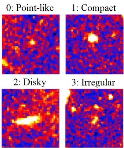
Figure 1. Example galaxies and their assigned visual classi-fications. Top left: 0 corresponds to point-like, a small point source. Top right: 1 corresponds to compact, an extended circu-lar source. Bottom left: 2 corresponds to disky, an extended oval or disk-shaped source. Bottom right: 3 corresponds to irregular, a clumped obscurely-shaped source with multiple components. There is no example of the−1 classification as these were unclas-sifiable and as such do not have a set morphology.

the source, such that the rest frame at our highest redshift (z_∼5.8) is_∼1197 ˚A and at the lowest (z_∼2.2) is_∼2528 ˚

A. Each of the galaxies in this reduced data set (known as

1000 Brightest, see Table 1) was then independently

clas-sified by three different team members in SAOImage DS9, using the same viewing settings. The classification scheme used split galaxies into four groups of decreasing

compact-ness (inspired by a similar method used inPaulino-Afonso

et al. 2018), with 0 as point-like, 1 as compact, 2 as disky

and 3 as an irregular/merger galaxy as shown in Figure1.

The additional classification of ₋1 was added for galaxies

it was not possible to classify on this scale, either because there was no image of the galaxy or the galaxy could not be seen in the image.

3.1.2 GALFITAnalysis of SC4K LAEs

We use results from Paulino-Afonso et al.(2018), in which the S´ersic profile was fitted to the observed light profile of

all of the 3908 galaxies in the SC4K data set using GALFIT

(Peng et al. 2002, 2010). This produced values for the

fit-ted half light radius (re), S´ersic index (n), observed 20%, 50% and 80% light radii (r20,r50andr80, the radii at which

20%, 50% and 80% of the observed light falls withinr,

re-spectively), and the compactness (C) of 3081 galaxies. While GALFITconverged for 3081 of the 3908 SC4K galaxies, a fur-ther 1478reandnvalues were removed under the conditions that 1₃ < re

r50 <3, which ensuresre is kept relatively close tor50, and thatn <10, as where this limit is exceeded it is

an indication that the fitting process has failed (the result-ing distribution of the data set can be seen in Table1). The remaining results were then used both in this form and, as in Section3.1.1, in a mean value per redshift slice (alongside a corresponding standard deviation).

3.1.3 Stellar Masses

In Santos et al. (in prep.) different magnitudes are trans-formed into flux densities, SED fitting is then used to fit this data with curves describing stellar population from which the stellar mass needed to produce said populations were then calculated. This paper uses a reduced set of this data by removing all AGN (by removing all X-ray and radio sources,

see Section3.2), which skew stellar mass measurements due

to their extra light output, and galaxies with stellar masses M such that Mstellar<8, where Mstellar= log10 MM

. This is because these values are numerical artefacts due to our data not being deep enough to detect such galaxies as they are not luminous enough. The mean stellar mass per redshift slice and corresponding standard deviation was then calcu-lated from the resulting data set (see Table1) as in Section 3.1.1.

3.2 X-ray and Radio: AGN

3.2.1 Determining AGN

An image of the entire COSMOS field was obtained as

viewed by the Chandra X-ray Telescope in three different

X-ray energy bands: 0.5₋2 keV (soft), 2₋7 keV (hard)

and 0.5−7 keV (full). As inSobral et al.(2018a), we follow

(Calhau 2019) and create cutouts of each object to then

cal-culate their X-ray fluxes, X-ray luminosities and black hole accretion rates (BHAR). The same method was then used on similar whole field images from the VLA radio observatory, with bands of 1.4 GHz and 3.0 GHz. The two new catalogues were then matched together, and the 303 objects which had been detected in any of the wavebands were marked as AGN. Note that there is some overlap - some objects were detected in multiple wavebands. An object was considered detected in a band if its signal was greater than 3 times the noise value, and the number of sources that fit this criteria in each band are given in Table2.

Each of these was visually inspected to determine which had visible jets, lobes or particularly bright centres in the X-ray and radio wavelengths. This was done by viewing a 15

arcsecond cutout image of each object in both radio wave-lengths (10 cm and 20 cm) and the soft X-ray energy band (0.5−2 keV), then combining these three images into one, with each wavelength being assigned to be either red, green or blue for added clarity. These colour images were then in-spected to identify key features. This process also revealed that two of the objects identified as AGN were the same object viewed in the SC4K sample through different filters, as explained inSobral et al.(2018a).

3.2.2 Calculating Black Hole Accretion Rate

To calculate the BHAR of the AGN, we follow Calhau

(2019), beginning with calculating the X-ray flux from the count rate, as in Equation2.

FX-ray= (counts/s)×CF×10−11(erg s−1cm−2) (2)

CF is a conversion factor with values of 0.687, 3.05 and 1.64 for the soft, hard and full X-ray bands respectively. These values were obtained by taking the average of the values given inElvis et al.(2009) and the more recent paperCivano

et al.(2016). From these fluxes we then calculate the

lumi-nosity with Equation3,

LX-ray= 4πFX-rayd2L(erg s−1) (3)

where dL is the luminosity distance in cm, converted from

the values given in Table3.

This then required correction by multiplying it by a K-correction factor and converting each band’s luminosity into the 0.5₋10 keV luminosity, as in Equation4:

L0.5−10keV=

LX-ray(10(2−Γ)−0.5(2−Γ))

(Emax(1 +z))(2−Γ)_{−(Emin(1 +z))}(2−Γ) (4)

where z is the redshift, Γ is the photon index assumed to

be 1.4 as in Calhau et al. (in prep.) and Emaxand Eminare

the maximum and minimum energies of each band. Before obtaining the BHAR, we must multiply our K-corrected luminosities by a bolometric correction value. This value is extremely variable, but we take it to be 22.4 as in

Lehmer et al.(2013a), as this is the median value for AGN

with LX-ray= 1041−1046erg s−1. The BHAR of our sources

can then be calculated using Equation5:

˙

MBH=(1−)L

AGN bol

c2 (5)

where ˙MBHis the BHAR in units of Myr−1, c is the speed of light andis the accretion efficiency, taken to be 0.1 as

inMarconi et al.(2004).

3.3 Calculating Star Formation Rates

There are a number of techniques and calibrations one can use to estimate the star formation rate (SFR) in distant galaxies. HII regions are created around O and B type stars when ultraviolet (UV) photons ionise the surrounding hydro-gen. When the ionised hydrogen ions recombine with elec-trons, they emit photons of characteristic frequency such

as Lyαand H-alpha (Hα). In this way we can measure the

number of photons and calculate the SFR in distant galaxies.

Ideally we would use the Hαline to measure instantaneous

Data Reduction Total Number Data Set

Set Conditions of Sources Used for

Full SC4K None 3908

1000 Brightest MBB<25.1974 1000 Cutouts

VC Mean Trusted MBB<25.1974, VC Mean>−0.5 788 VC Mean

GALFITOutput GALFITConverges 3081 r20,r50,r80, C

S´ersic Trusted GALFITConverges, 1₃< re

r50 <3,n <10 1603 re,n

Mass Trusted Mstellar>8 3425 Mstellar

Redshift Full SC4K VC Mean Trusted GALFITOutput S´ersic Trusted Mass Trusted

z Sources (%) Sources (%) Sources (%) Sources (%) Sources (%) 2.22 4.1±0.3 5.8±0.9 4.3±0.4 3.4±0.5 1.8±0.2 2.51 19.0±0.8 18.8±1.7 19.4±0.9 20.1±1.2 19.6±0.8 2.82 8.0±0.5 11.5±1.3 7.7±0.5 7.6±0.7 8.3±0.5 2.98 18.2±0.7 11.3±1.3 18.5±0.8 18.3±1.2 18.9±0.8 3.12 1.15±0.17 2.2±0.5 1.4±0.2 1.1±0.3 0.76±0.15 3.15 12.4±0.6 18.4±1.7 12.3±0.7 13.3±1.0 13.2±0.7 3.33 16.4±0.7 15.5±1.5 16.6±0.8 16.8±1.1 17.3±0.8 3.72 2.5±0.3 4.6±0.8 2.5±0.3 2.7±0.4 2.7±0.3 4.13 3.6±0.3 1.8±0.5 3.7±0.4 3.8±0.5 3.9±0.3 4.58 2.0±0.2 1.5±0.4 2.2±0.3 2.1±0.4 1.9±0.2 4.83 2.1±0.2 2.9±0.6 2.0±0.3 1.9±0.3 2.3±0.3 4.85 2.0±0.2 1.3±0.4 1.9±0.3 1.9±0.4 2.1±0.2 5.07 2.0±0.2 2.8±0.6 2.0±0.3 2.0±0.4 2.0±0.2 5.31 0.84±0.15 1.0±0.4 0.78±0.16 0.7±0.2 0.88±0.16 5.71 4.9±0.4 – 4.8±0.4 3.6±0.5 3.8±0.3 5.80 0.90±0.15 0.5±0.3 0.75±0.16 0.50±0.18 0.67±0.14

Table 1.The reduction conditions used in Section3.1on the SC4K catalogue and the number of sources in the data sets produced, includ-ing the percentage of each data set’s total number of sources in each redshift slice Percentage =_{Total Number of Sources for this Data Set}Number of Trusted Sources in Slice

. WhereMBBis the broad band magnitude of the galaxy (note, this will range from u and B to i and z bands) and VC Mean is its mean visual classification. The – in the VC Mean Trusted column is due to a lack of any sources for this redshift slice.

Waveband Number of Detected Sources Detected Sources (%)

1.4GHz 54 1.38

3.0GHz 84 2.15

Soft 235 6.01

Hard 206 5.27

Full 223 5.71

Table 2.The number of sources with a signal value greater than 3 times that of the noise value in each waveband. 1.4GHz and 3.0GHz are the radio wavebands, and Soft, Hard and Full are the X-ray wavebands with energies of 0.5−2 keV, 2−7 keV and 0.5−7 keV respectively as described in Section3.2.1.

z_∼2.5, and hence we cannot observe it using ground based

telescopes. Future work (when the JWST launches) will be

able to calculate SFRs at high redshift using the Hα line,

which can then be compared to that of Lyα.

In this paper, we use Lyαluminosities, rest-frame UV

magnitudes, along with radio and far infrared (FIR) stacking to calculate SFRs. Each of these processes traces a different aspect of star formation, and thus gives different implica-tions for SFRs.

The first step in making use of the data was to reduce the relevant catalogues to only those sources not affected by AGN. This is because the accretion disks of AGN emit photons across a range of frequencies, some frequencies to a greater extent than others (e.g. radio and Lyα) – see Section

4.2– and would therefore produce seemingly high SFR

val-ues and contaminate the results if included. We eliminated all possible AGN by excluding all sources that were detected to emit significantly in either radio and/or X-ray (as detailed in Section3.2), which are clear indicators for AGN activity. Despite the FIR data not being so affected by AGN emis-sions – as FIR traces dust-obscured SFRs (Calhau et al. in prep.) – excluding them meant that the subsequently ob-tained SFRs from FIR stacking could be compared alongside those from radio.

The methodologies behind Lyα luminosity and UV

magnitude results are covered in Section3.3.1 and Section

3.3.2, respectively, and those for radio and FIR stacking are

detailed in Section3.3.3and Section3.3.4, respectively.

3.3.1 Lyman-alpha

Lyαis emitted from ionised gas around star forming regions

and AGN, and therefore traces O and B type stars (M≥10

M) with lifetimes of the order of_∼Myrs. Hence, Lyαcan

give an excellent indication of the instantaneous SFR in a

galaxy. However, a significant fraction of Lyα photons are

scattered by the interstellar medium (ISM) leading to kpc-long random walks. As a consequence, there is a very high

probability that Lyα photons are absorbed by dust

parti-cles and destroyed. This leads to the amount of photons we receive being lower than expected, resulting in lower calcu-lated SFRs (Sobral & Matthee 2019).

109 emitted strongly in the X-ray, and 62 emitted strongly in the radio. 142 sources emitted strongly in either or both,

leaving 3766 sources available for us to investigate Lyα

SFRs. Some of the average properties of this sample are presented in Table3.

We follow Sobral & Matthee(2019) for the dust cor-rected SFR, in Myr−1_{, based on Kennicutt(1998) and a}

Salpeter IMF (0.1−100 M) using Equation6:

SFRLyα=

LLyα×7.9×10−42 (1₋fesc,LyC)(0.042EW0)

(_±15%) (6)

where LLyα is the Lyα luminosity, EW0 is the rest frame

equivalent width, andfesc,LyC is the Lyman continuum

es-cape fraction. We assume thatfesc,LyC= 0.

Once we had obtained individual SFRs for each source, we averaged the SFR of all sources in each redshift bin, in order to obtain an average SFR per redshift bin, with associ-ated standard deviations on both the SFR and the redshift. The redshift bin allocations are outlined in Table3.

We found that the average SFRLyα was 16.5±0.3

Myr−1_{, with a standard deviation of 21.0 M}

yr−1 over

the 3766 sources.

3.3.2 Rest-frame Ultraviolet

Younger and more massive stars (O and B type) emit strongly in the UV, and in a similar fashion to Lyα, we can use rest frame UV magnitudes to calculate instantaneous

SFRs. Sobral et al. (2018b) gives the UV SFR in Myr−1

using Equation7:

SFRUV= (1.4×10−28)4π×9.521×1038×10−0.4(MUV+48.6)

(7)

where the absolute UV magnitudeMUV is calculated using

Equation8:

MUV=mUV−5log10

_d

L

10 pc

+ 2.5log₁₀(1 +z) (8)

where we use the rest frame B band from SED fitting as in

Ilbert et al.(2009) formUV , and dL is the luminosity

dis-tance. Note that we use the B band as inIlbert et al.(2009)

formUV across the whole redshift range, but this method

will become less accurate as we move to higher redshifts, as the wavelength we observe the rest frame to be at increases. Future work to improve on this would be to use different bands for different redshifts.

In the same way as for Lyα, we averaged individual

SFRs over the redshift bins outlined in Table 3. We found

that the average SFRUVto be 4.55 Myr−1with a standard deviation of 4.73 Myr−1across 3766 sources.

3.3.3 Radio

We made use of data from radio stacking; a technique in which data from many individual objects is combined in order to determine the average properties of sources that are too faint to be detected individually. Stacked values of certain average galaxy properties, such as flux densi-ties, fromCalhau(2019) were used for given redshifts. The stacking process results in these values being upper limits, rather than direct measurements. Once the determined AGN

sources were removed from the data set, leaving only non-detections, the luminosity distance dL of each redshift bin

was calculated from the medianz value. This was done

us-ing a calculation followus-ing Hogg (1999), with the Hubble

constantH0and energy density distributions stated in

Sec-tion1. The obtained dLvalues (used for both radio and FIR

stacking methods) are presented in Table3.

FollowingCalhau(2019), the upper limits of flux den-sities for 1.4 GHz were used to determine the upper limits of luminosities L1.4GHz in WHz−1 using Equation9,

L1.4GHz= 4πd2LS1.4GHz×10−33(1 +z)α−1 (9)

where dLis the luminosity distance in cm, S1.4GHzis the flux

density at 1.4 GHz in mJy,zis redshift andαis the the radio

spectral index, assumed to be 0.8 (Delhaize et al. 2017).

Often, a similar process is also carried out for frequency 3.0 GHz as this probes deeper still than 1.4 GHz. In this work, however, we focus just on 1.4 GHz radio luminosity. The upper limits of SFR1.4GHz, in Myr−1, could then be

calculated from the obtained luminosities followingCalhau

(2019) (submitted) using Equation10(Karim et al. 2011).

SFR1.4GHz= 3.18×10−22L1.4GHz (10)

These values are for a Chabrier IMF and as such were later scaled by a factor of 7.9

4.4 to a Salpeter IMF for

com-parison with the values obtained through the methods

out-lined in Section 3.3.1. The SFR upper limits calculated

(103 Myr−1

. SFR1.4GHz . 2440 Myr−1) are discussed in further detail in Section6.2.

3.3.4 Far Infrared

Similarly to the process carried out for radio stacking, SFR upper limits were determined using stacked FIR data from

Calhau(2019). The original flux density limits (actually 3_×

noise, rather than “data points”) in the catalogue were in units of Jy and first had to be converted into flux densities per wavelength. Once this was done, the flux densities for each redshift were plotted against rest frame wavelength,λ0,

which were calculated from the observed wavelengths,λobs,

provided in the data catalogue using the relation given by Equation11.

λ0= λobs

(1 +z) (11)

To obtain the upper limits of total flux across the FIR wavelength range, the flux densities were also converted into rest frame values by multiplying them by a factor of (1 +z) before integrating. As all that was available was the given flux density values, the functional form of this plot was unknown. This was approximated as a Planck black body

curve, shown by Equation 12, which was manually

modi-fied in each case to best fit the upper limit values. This approximation can be made as FIR emissions are due to the absorption of UV radiation by dust in HII regions and its subsequent re-emission in the far infrared range after the de-excitation of the heated dust particles. This black-body-like radiation corresponds to a temperature in the range

∼20₋80 K.

The method used is a simplified form of spectral energy

distribution (SED) fitting and an example for z _∼ 3.3 is

Filter λc Average LLyα Average Mass Bin No. Sources z1.4GHz,FIR dL

[˚A] [log10(erg s−1)] [log10(M)] [104Mpc]

NB392 3920 42.6 9.22 z∼2.2 146 2.51 2.05

IA427 4270 42.7 9.09 z∼2.5 714 2.82 2.35

IA464 4640 42.9 9.16 z∼3.1 293 2.98 2.52

IA484 4840 42.9 9.12 z∼3.1 673 3.15 2.70

NB501 5010 43.0 9.38 z∼3.1 39 3.33 2.88

IA505 5050 42.9 9.28 z∼3.1 467 3.72 3.29

IA527 5270 42.9 9.27 z∼3.1 626 4.13 3.72

IA574 5740 43.0 9.38 z∼3.9 96 4.58 4.21

IA624 6240 43.0 9.22 z∼3.9 141 4.83 4.48

IA679 6790 43.3 9.42 z∼4.7 76 5.07 4.74

IA709 7090 43.19 9.29 z∼4.7 80 5.31 5.00

NB711 7110 42.8 9.10 z∼4.7 78 5.71 5.45

IA738 7380 43.27 9.46 z∼5.4 78 – –

IA767 7670 43.4 9.48 z∼5.4 32 – –

NB816 8160 42.9 9.40 z∼5.4 192 – –

IA827 8270 43.5 9.69 z∼5.4 35 – –

Table 3.The redshift bin allocations for our sample (Sobral et al. 2018a).z1.4GHz,FIRare the median redshift values from the stacked radio and FIR data (Calhau et al. in prep.) detailed in Section3.3.3and Section3.3.4and correspond to luminosity distances dL. The – is due to lack of values.

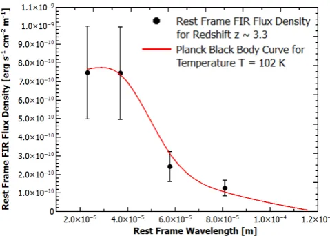
Figure 2. The rest frame FIR flux density (3×noise) against rest frame wavelength for z ∼ 3.3. The red curve is a Planck black body curve, given by Equation12for temperature T = 102 K, with its amplitude modified to best fit the flux density limits. This temperature is higher than might be expected (on the order of∼10 K) but this is due to the limitations of the black body approximation. The value of T was chosen in each case to fit the values, rather than directly corresponding to the properties of the emission. Another potential SED fitting approach to improve on this is to make the “greybody” approximation discussed inCasey

(2012) but not applied in this work.

This curve was then integrated with respect to wave-length, providing the upper limit of total flux for the given rest frame wavelength range.

Bλ(λ,T) =2hc

2

λ5

1

exp( hc

λkBT)−1

(12)

Bλis the spectral radiance for wavelengthλ, T is the tem-perature,his Planck’s constant, andkBis Boltzmann’s

con-stant. From the flux obtained through the integration of this function, luminosities LFIRcould then be calculated in units

of erg s−1 using Equation13,

LFIR= 4πd2LfFIR (13)

where dLis the luminosity distance in cm and fFIRis the flux

in erg s−1_cm−2_{. SFR}

FIR values, in Myr−1, could then be calculated from the luminosities obtained using the relation given inKennicutt(1998), as displayed by Equation14.

SFRFIR= 4.5×10−44LFIR (14)

The SFR upper limits determined from FIR stacking data (68.4 Myr−1

. SFR1.4GHz .1820 Myr−1) are dis-cussed in Section6.2.

3.3.5 Star Formation Rate Density

Star formation rate densities (SFRDs) are essentially the amount of stars forming per unit co-moving volume. It is important to note that the SFRDs in this paper were calcu-lated differently to the SFRs. To determine the LyαSFRD in Myr−1_Mpc−3_{, we followSobral et al.(2018a) using}

Equa-tion15:

SFRDLyα=

ρLyα×7.9×10−42 (1₋fesc,LyC)×0.042EW0

(15)

whereρLyα is the Lyαluminosity density. We followSobral

et al.(2018a) in derivingρLyαby integrating the Lyα

lumi-nosity function for each redshift slice in the SC4K sample. To determine the UV SFRD, we took the rest frame UV SFRs calculated previously as in Section3.3.2, and pro-duced histograms of the weighted count of each galaxy with a certain SFR for each redshift bin. The weighted count n was calculated by dividing the number of sources N by the co-moving volume of the redshift slice V multiplied by the

width of the SFR bin (∆SFR), as shown in Equation16.

n = N

Figure 3.Determining n* and SFR*, which when combined in Equation17can be used to calculate SFRDUV.

Visual VC Percentage of

Classification Mean Sources (%)

Point-like −0.5<VC Mean<0.5 19.7±1.7 Compact 0.5<VC Mean<1.5 39±3

Disky 1.5<VC Mean<2.5 30±2 Irregular 2.5<VC Mean<3 11.3±1.3

Table 4.The distribution of the VC Mean Trusted data set (Ta-ble1, Section3.1) over the classification scale described in Section

3.1.1.

An approximate Schechter function was fitted manually to each histogram, where the ‘typical’ SFR (SFR*) and ‘typi-cal’ number density (n*) could be approximated. Then,

us-ing Equation 17, the UV SFRD was calculated. The errors

in SFRDUV, in Figure15, are proportional to the confidence

in which we determined n* and SFR* using the histograms.

An example is shown in Figure3.

SFRDUV=

Z

ΦdSFRD = SFR∗_×n∗_×Γ(α+ 2) (17)

Φ is the Schechter function and Γ is the error function. We useα= -1.8.

4 RESULTS

4.1 Morphologies

4.1.1 Visual Classifications

Of the 788 galaxies in the reduced data set, most fell into

the compact and disky ranges (see Table 4 for percentage

distributions) while the average value across all redshifts is 1.3_±0.8. There is some fluctuation of visual classification mean (VC Mean) per redshift about this value which can

be seen in Figure4, with VC Mean per redshift starting at

0.17±0.17 at redshift 5.8, climbing to 1.7±0.9 at redshift 4.1 before declining to 0.8_±0.8 at redshift 2.2. See Table5 for more detail.

4.1.2 GALFITAnalysis of SC4K LAEs

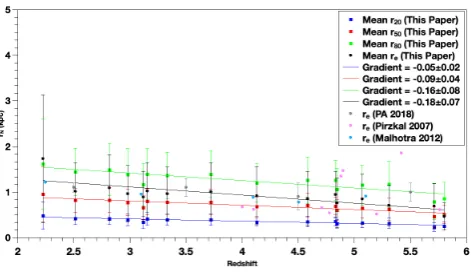
As can be seen in Figure 5, there is a tentative increase

in all measurements of galactic radius with age (increase

Figure 4. Mean visual classification per redshift slice against redshift, with standard deviation errors in which the majority of data points lie in the 1<VC Mean<2 range (compact to disky).

in r20 = 0.05 ± 0.02 kpc per unit redshift, increase in r50 = 0.09±0.04 kpc per unit redshift, increase in r80 =

0.16_±0.08 kpc per unit redshift and increase inre= 0.18± 0.07 kpc per unit redshift) with the 50% to 80% light radii range increasing∼1.75 times faster than that of the 20% to

50% range. Our results agree well with those of

Paulino-Afonso et al. (2018), Pirzkal et al. (2007) and Malhotra

et al.(2012) in that, while there is a minor increase of radii

with cosmic time, this is ∼ 2σ and is around an average

radius of_∼1 kpc. The S´ersic index has an overall mean of

1.9_±2.2 (this large error is due to the wide range ofnvalues, 0< n < 10, despite 50% of alln values falling between 0

and 1.5) this is consistent withz_∼2₋6 SC4K LAEs being

on average compact disks (which haven∼2) from Section

4.1.1. Figure 6shows a similar pattern to Figure4, if to a

lesser extent (and within error bars), of starting low (0.9±0.7 at redshift 5.8), increasing so that most meannper redshift slice value lie above the fitted line and then decreasing again (to 1.4_±1.8 at redshift 2.2). The overall mean compactness is 2.6_±0.4 and this stays consistent over time (with a rate of change of−0.00±0.07 per unit redshift) within the stan-dard deviation. This result, and that of the S´ersic index data are consistent with results fromPaulino-Afonso et al.(2018)

which found a mean compactness C_∼2.7, and S´ersic index

n.2.

4.1.3 Stellar Masses

Figure 7 shows a tentative decrease in mass with age at

a rate of 100.09±0.05 _M

per unit redshift. Also shown in

Figure7are the Mstellarvalues fromPirzkal et al.(2007) and

Shapley et al.(2005), our data does not fit well with most

of theShapley et al.(2005) data and all but one data point

fromPirzkal et al.(2007) which predict a gradient opposite

Redshift VC Mean r20 r50 r80 C re n Mstellar

z (kpc) (kpc) (kpc) (kpc) (log₁₀(M))

2.22 0.8±0.8 0.5±0.3 1.0±0.6 1.6±1.0 2.6±0.4 1.7±1.4 1.4±1.8 9.2±0.6 2.51 1.3±0.8 0.42±0.13 0.8±0.3 1.4±0.5 2.6±0.4 1.0±0.6 2±2 9.1±0.6 2.82 1.3±0.7 0.42±0.13 0.8±0.3 1.5±0.6 2.7±0.4 1.1±0.7 2±2 9.2±0.5 2.98 1.4±0.8 0.39±0.13 0.8±0.3 1.4±0.6 2.7±0.4 1.0±0.6 2±2 9.1±0.6 3.12 0.9±0.6 0.34±0.13 0.7±0.3 1.2±0.5 2.6±0.4 0.9±0.6 2±2 9.4±0.5 3.15 1.6±0.8 0.41±0.14 0.8±0.3 1.4±0.6 2.6±0.4 1.0±0.6 2±2 9.3±0.6 3.33 1.3±0.9 0.40±0.12 0.8±0.3 1.4±0.5 2.6±0.4 1.0±0.6 2±2 9.3±0.6 3.72 1.4±0.9 0.39±0.13 0.8±0.3 1.4±0.5 2.7±0.4 1.0±0.6 3±3 9.4±0.5 4.13 1.7±0.9 0.35±0.09 0.7±0.2 1.2±0.4 2.6±0.4 0.9±0.6 2.0±1.8 9.2±0.6 4.58 1.2±0.7 0.35±0.11 0.7±0.3 1.3±0.5 2.7±0.3 0.9±0.6 2±2 9.4±0.5 4.83 1.3±0.8 0.36±0.10 0.69±0.19 1.3±0.4 2.7±0.4 0.9±0.5 2±2 9.3±0.5 4.85 1.2±0.8 0.31±0.10 0.6±0.2 1.1±0.5 2.6±0.4 0.8±0.5 1±3 9.1±0.5 5.07 1.0±0.8 0.32±0.11 0.7±0.2 1.2±0.4 2.7±0.4 0.9±0.5 3±3 9.5±0.4 5.31 0.9±0.6 0.32±0.12 0.6±0.2 1.2±0.5 2.8±0.5 0.7±0.5 2.1±1.5 9.5±0.2 5.71 – 0.24±0.10 0.5±0.2 0.8±0.4 2.5±0.5 0.7±0.5 2±2 9.4±0.4 5.80 0.16±0.16 0.25±0.09 0.5±0.2 0.9±0.4 2.5±0.4 0.5±0.3 0.9±0.7 9.7±0.3

Table 5.The mean values and standard deviation per redshift slice of the reduced data sets (see Table1) considered in this study. VC Mean is the mean visual classification (0 being point-like, 1 is compact, 2 is disky and 3 is irregular, see Section4.1.1for more details on these results).r20,r50,r80andreare the 20%, 50%, 80% and fitted half light radii (the radii at which 20%, 50%, 80% and half the

light falls within said radius), and C andnare the compactness and the S´ersic index respectively (see Section4.1.2for more on these results). Mstellaris the logged stellar mass of the LAE (see Section4.1.3for more on these results). The – in the VC Mean column is due to a lack of any sources for this redshift slice, as in Table1.

Figure 5. The sizes of our LAEs as a function of redshift for different radii (rN) and their standard deviations, where dark blue isr20, red isr50, green isr80and black isrewhich are the

radii at which 20%, 50%, 80% and half the light falls within said radius, respectively (see Section3.1.2). Also shown arere data

fromPaulino-Afonso et al.(2018) in grey,Pirzkal et al.(2007) in pink, andMalhotra et al.(2012) in light blue.

4.2 AGN

From theChandraand VLA data, 303 AGN sources in the

SC4K catalogue were identified, 240 of which are detected at X-ray wavelengths and 119 are detected in the 1.4 GHz and 3.0 GHz radio bands combined. For all sources detected in the X-ray wavelength the luminosities calculated where found in a range between_∼1042_{erg s}−1 _and

∼1045_{erg s}−1_.

These luminosities correspond to a range of black hole accre-tion rates (BHAR) from_∼0.03 Myr−1 _to

∼3.3 Myr−1_,

which is consistent with the range of BHARs expected across this redshift range (e.g. Calhau 2019; Shields 1999). Two AGN were also found to have much larger BHARs of

Figure 6.Mean S´ersic index and standard deviation per redshift slice against redshift showing no evolution which is consistent with our LAEs on average compact disks (n∼2) fromz∼2−6.

(6.9_±2.3) Myr−1 _{and (10.0}

±0.1) Myr−1_{, indicating}

highly active AGN in our sample.

The fractions of AGN in the SC4K catalogue across the

range of Lyα luminosities and across the redshift range of

the catalogue are plotted (see Section4.2.1and Section4.2.2 respectively) and the trend in the relation between BHAR and the morphologies of the AGN in our catalogue (shown in Section4.2.3) is explored, in order to investigate the lu-minosity, size and evolutionary trends of the AGN identified in the SC4K catalogue.

4.2.1 AGN Activity Dependence on Lyman-alpha Luminosity

Figure 7.Graph of mean stellar mass and standard deviations per redshift slice against redshift. Where navy is Mstellar from this paper, pink is MstellarfromPirzkal et al.(2007), and orange is MstellarfromShapley et al.(2005).

LLyα∼1042.4 erg s−1 which is consistent with the expected Lyαluminosities of our AGN (e.g.Calhau 2019).

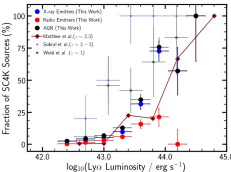
Plotting the fraction of all active galaxies in our cata-logue, those which are X-ray or radio emitters and the

com-bined fraction, against the Lyα luminosity (see Figure 8)

shows that the fraction of all galaxies which are AGN in-creases rapidly with the luminosity, with only a small frac-tion at_∼1042_{, increasing almost exponentially as}

luminos-ity increases up to ∼1045. This trend is in agreement with that found inMatthee et al.(2017), shown on Figure8, and shows a similar AGN fraction to that found with spectro-scopic data taken in Sobral et al.(2018b) andWold et al. (2014).

Whilst there is a general increase in the fraction of sources emitting in X-ray or Radio, which flows the trends found in previous studies, it can be seen that the fraction of sources emitting in the Radio range is consistently lower than that of the fraction emitting X-rays. This difference becomes more pronounced at higher luminosities.

At high luminosities the sample size is small which may cause the results to be skewed due to sample bias, which causes the uncertainties on the AGN fraction to increase

with the Lyαluminosity of the AGN.

4.2.2 Redshift Dependence of AGN Fraction

Plotting the fraction of AGN in our catalogue at different redshift bins shows that the fraction of AGN remains rela-tively low, remaining below 15% of the total sources, across the range of the catalogue with only slight fluctuations (see Figure9), following a similar trend to that found in previous studies such asCalhau(2019) andLehmer et al.(2013a).

As shown in Figure9, the fraction of radio sources shows a gradual increase as the redshift value decreases, peaking

slightly atz _∼3₋4 before decreasing again fromz _∼3 to

z∼2. The fraction of X-ray AGN in our catalogue shows a

similar yet less distinct trend with redshift, whilst peaking atz∼3 andz∼5.5. From the fraction of AGN in the red-shift ranges ofz_∼2₋4 andz_∼4₋6 the overall decrease in the source fraction with redshift can been seen, with the percentage fractions of X-ray, radio and the combined AGN fraction given in Table6.

Figure 8.The faction of X-ray AGN (blue), radio AGN (red) and the combined AGN fraction (black) in the SC4K catalogue, in luminosity LLyα bins of 100.3 erg s−1, showing the rapid

in-crease in the fraction of AGN as the luminosity inin-creases. Similar results have been found in previous studies,Matthee et al.(2017) (maroon) is show here with our data. For comparison we also show the AGN fractions found using spectroscopic data across redshifts ofz∼1 (grey) andz∼2−3 (lilac) fromSobral et al.

(2018b);Wold et al.(2014) respectively.

LAEs z∼2−4 fraction z∼4−6 fraction

[%] [%]

Total in Catalogue 81.6±0.6 18.4±0.6 X-ray emitters 6.9±0.4 2.8±0.6 Radio emitters 3.4±0.3 1.3±0.4 AGN (X-ray+Radio) 8.7±0.5 3.6±0.0 Table 6.The fraction of X-ray AGN, radio AGN and the com-bined total AGN fraction in the redshift ranges ofz∼2−4 and

z∼4−6 showing the overall decrease in AGN fraction with the increase in redshift. The fraction of all sources in each redshift range is also shown.

Thus the AGN fraction in each redshift bin decreases

with an increase in redshift, peaking at cosmic noon (z _∼

2−3), as has been observed in previous studies (e.g.Calhau 2019). The peak observed at the redshift ofz_∼5 is likely due to sample bias as only brighter LAEs are detected at high redshifts which are found to be mostly AGN (see Section

4.2.1), and the sample size at higher redshifts is small.

4.2.3 Morphological Trends in SC4K AGN

From the morphology calculations the light radii of the galaxies in our catalogue have been found (detailed in

Sec-tion3.1). This allows the morphological trends of the AGN

in the range ofz _∼2₋6 to be investigated. From our 303

AGN sources, only 198 had percentage light radii calculated and only 53 have S´ersic indices which could be calculated to a reasonable degree of accuracy (see Table1).

Figure 9.The fraction of X-ray AGN (blue), radio AGN (red) and the combined AGN fraction (black) in the SC4K catalogue, in redshift bins of 0.3 (indicated by the errors in redshift), showing two slight peaks at z ∼ 3 and z ∼ 5 and an overall gradual downward trend in the AGN fraction. The binomial errors in the fraction of sources detected are shown.

50% and 80% light radii, shows the spread of AGN sizes, see

Figure 11, with most of the light being emitted about the

central region within which is the supermassive black hole. 80% of the light emitted by the whole active galaxy is within ∼4.5 kpc of the centre, with 50% of the light emitted within ∼3.0 kpc and 20% emitted within∼2.0 kpc of the centre of the AGN. From the spread of the data points it can be seen that the most active sources, for which the percentage light radii have been calculated, typically have smaller light radii at each percentage, with the percentage light radius de-creasing with the increase in BHAR. Plotting the half light radii calculated using the S´ersic profile (see Section 3.1.2) of our AGN, against the BHAR values shows that the half light radius decreases rapidly, from a radius of_∼4.75 kpc

to a radius of∼0.1 kpc, with increasing BHAR. Thus most

light emitted by active galaxies is produced by the super-massive black hole in the centre of these galaxies, with the more active AGN being more luminous in the central region the galaxy.

From the visually classified morphologies (see Section

3.1.1) the fraction of AGN in our catalogue with the

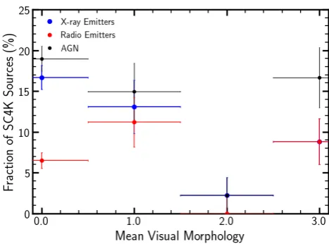
differ-ent visual morphologies shows that a greater percdiffer-entage of AGN have visual morphologies of 0 and 1, with the X-ray and radio fractions peaking a visual morphologies of 0 and 1 respectively (see Figure10). A slight peak in the AGN frac-tion also occurs for a visual morphology of 3. Thus AGN are typically more point-like compact sources with some appear-ing as more irregular sources, which is consistent with what we expect. This concurs with the half light radii, from the S´ersic profiles, and the percentage light radii results, indicat-ing AGN typically appear as very bright point-like sources, with little of the surrounding galaxy visible due to the high luminosity of the supermassive black hole itself.

Figure 10. The fraction of X-ray (blue), radio (red) and the combined AGN fraction (black) with visual morphologies of 0, 1, 2 and 3, corresponding to point-like, compact, disky and irregular morphologies respectively, showing a peak in the fraction of AGN at point-like and compact morphologies and again for irregular morphologies. This is likely due to the compact nature of the bright centres of Active Galaxies and the radio jets that can be detected from AGN.

Figure 11.The 20% (red), 50% (Purple) and 80% (blue) light radii, against the BHAR with AGN of higher BHAR having smaller percentage light radii. From the scatter the range of light radii at 20%, 50% and 80% can be seen as ∼ 0.1−0.5 kpc,

∼0.5−1.0 kpc and∼1.2−3.0 kpc respectively.

4.3 SFR

Figure12(bottom right panel) shows that SFR is generally

greater at higher redshifts, except at redshifts z & 5. Be-tween redshifts 4.8₋5, we no longer see SFR increase with

increasing z. Instead, the results show that a given SFR

occurs at a higher stellar mass M. Across the stellar mass range, we see a local maximum in SFR for each redshift slice. Averaged across the redshift range, this local maximum is located at M_∼109.3 _M

lo g 1 0 (S F R [ M ⊙ y r -1]) −1 −0.5 0 0.5 1 1.5

log10(Stellar Mass [M⊙])

8 8.5 9 9.5 10 10.5 11

z ∿ 2.5

z ∿ 2 Dutton et al. (2009)

lo

g10

(S F R [ M⊙ y r -1]) −0.5 0 0.5 1 1.5 2

log10(Stellar Mass [M⊙])

8 8.5 9 9.5 10 10.5 11 z ∿ 3.1

z ∿ 3 Dutton et al. (2009)

lo

g10

(S F R [ M⊙ y r -1]) 0.6 0.8 1 1.2 1.4 1.6 1.8 2

log10(Stellar Mass [M⊙])

8.5 9 9.5 10 10.5 11 z ∿ 4

z ∿ 4 Salmon et al. (2014)

lo g 1 0 (S F R [ M ⊙ y r -1]) 0.8 0.9 1 1.1 1.2 1.3 1.4 1.5 1.6 1.7

log10(Stellar Mass [M⊙])

8 8.5 9 9.5 10 10.5 11

z ∿ 4.8

z ∿ 5 Salmon et al. (2014)

lo g 1 0 (S F R [ M ⊙ y r -1]) 0.9 1 1.1 1.2 1.3 1.4 1.5 1.6 1.7

log10(Stellar Mass [M⊙])

8 8.5 9 9.5 10 10.5 11 11.5 12

z ∿ 5.5

z ∿ 6 Salmon et al. (2014)

lo g 1 0 (S F R [ M ⊙ y r -1]) 0.6 0.8 1 1.2 1.4 1.6 1.8

log10(Stellar Mass [M⊙])

8 8.5 9 9.5 10 10.5 11 11.5

z ∿ 2.5 z ∿ 3.1 z ∿ 4.0 z ∿ 4.8 z ∿ 5.5

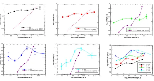
Figure 12.Ly↵SFR evolution with stellar mass for varying redshift bins. Top left:z⇠2.5; top middle:z⇠3.1; top right:z⇠4.0; bottom left:z⇠4.8; bottom middle:z⇠5.5; bottom right: combined results for all redshifts. Results fromDutton et al.(2010) and

Salmon et al.(2015) are plotted for redshifts z⇠2.5 3.1 and for redshiftsz⇠4.0 5.5, respectively. We find that in general SFR increases with stellar mass, and that SFRs are generally higher at higher redshifts. See Section6.2for further analysis.

we see that this maximum appears to progressively shift

to higher M with increasing z, peaking at M ⇠ 1010 M

forz ⇠5.5. The amplitude of these maxima are also seen to increase with increasing redshift. Atz ⇠ 2.5, the peak is at SFR⇠101.0 _{M yr} 1_{, but is located at SFR⇠10}1.6

M yr 1 _{for z ⇠ 5.5. However, the range of SFRs seems}

fairly consistent across the redshift range. Atz ⇠ 2.5, the range of SFRs is⇠100.4_{M yr} 1_{, but atz⇠5.5 the range}

is⇠100.5 _{M yr} 1_.

From redshifts z⇠ 2.5 4 we see that SFR increases

up to the maximum, dips briefly, then continues to increase again after the local maximum. However, at higher redshifts

(z ⇠4 5.5) we see SFR decrease after the ‘bump’. This

is most likely due to the ‘dust wall’ created by galaxies with large stellar masses and high SFRs. This a↵ects the Ly↵escape fraction, and hence directly a↵ects the SFR we calculate. According to Figure 13, this ‘dust wall’ occurs at SFRs greater than⇠ 101.6 M yr 1, and stellar masses greater than⇠1010_{M .}

Figure13shows that, averaged across the redshift range

z ⇠ 2 6, SFR increases with stellar mass, with further

results on the evolution of SFR with redshift presented in Figure14. In Figure13 we also see more clearly that the local maxima appear around a stellar mass of⇠109.3 _M

for both Ly↵and UV. Given this, and that the shape of the curves are practically the same, SFRLy↵ and SFRUV are

consistent, but di↵er in their scaling. The scaling di↵erence gives an indication of the dust content and the ionisation rate around the galaxies. This relationship is represented

by the ratio SFRLy↵/SFRUV, also shown in green in Figure

13. This ratio peaks at M ⇠ 1010 M , which is also the point where we found the ‘dust wall’ to become significant.

Figure14shows that, across all our data, observational SFRs tend to increase with redshift. Specifically, we find that

d dzlog10(

SFRLy↵

M yr 1) = 0.140±0.004, and _dzdlog10(_{M yr}SFRUV1) =

0.099±0.004. This demonstrates that SFRLy↵diverges from SFRUV, which is due to the presence of dust and a

vary-ing ionisation rate. Radio data provides upper limits on the SFR, and it is therefore in line with expectation that they form the ‘ceiling’ values in Figure14. As with Ly↵and UV, SFR1.4GHz increases with redshift. No line of best fit was

plotted because theses results are from non-detections. FIR data are also upper limits, and combined with UV would roughly trace the SFR given by radio stacking, and therefore give the total SFR, as FIR traces obscured star formation and UV traces unobscured.

In Figure14, the errors on redshift, SFRLy↵and SFRUV

are standard errors, calculated from the standard deviation. If error bars cannot be seen on SFRLy↵ and SFRUV, it is

because they are contained within the points themselves. The errors on the SFRFIRresults were derived from

un-certainties on the calculated fFIR upper limits. These were

determined by fitting and integrating two black body curves – the best and least acceptable fits – to the flux density up-per limits (3⇥noise from stacking) for each redshift. The di↵erence between the fFIR value obtained from each

inte-gration was taken to be the error on the flux limit in each case. The fractional error in each case was equated to the

LancAstro1,1–20(2019) Figure 12.LyαSFR evolution with stellar mass for varying redshift bins. Top left: z∼2.5; top middle:z∼3.1; top right:z∼4.0; bottom left:z∼4.8; bottom middle:z∼5.5; bottom right: combined results for all redshifts. Results fromDutton et al.(2010) and

Salmon et al.(2015) are plotted for redshifts z∼2.5−3.1 and for redshiftsz∼4.0−5.5, respectively. We find that in general SFR increases with stellar mass, and that SFRs are generally higher at higher redshifts. See Section6.2for further analysis.

this maximum appears to progressively shift to higher M with increasingz, peaking at M_∼1010_M

forz∼5.5. The amplitude of these maxima are also seen to increase with increasing redshift. Atz _∼2.5, the peak is at SFR_∼101.0

Myr−1, but is located at SFR∼101.6 Myr−1forz∼5.5. However, the range of SFRs seems fairly consistent across the redshift range. Atz∼2.5, the range of SFRs is∼100.4 Myr−1_{, but atz}

∼5.5 the range is_∼100.5_M

yr−1.

From redshifts z _∼ 2.5₋4 we see that SFR increases

up to the maximum, dips briefly, then continues to increase again after the local maximum. However, at higher redshifts

(z _∼ 4₋5.5) we see SFR decrease after the ‘bump’. This

is most likely due to the ‘dust wall’ created by galaxies with large stellar masses and high SFRs. This affects the

Lyαescape fraction, and hence directly affects the SFR we

calculate. According to Figure 13, this ‘dust wall’ occurs

at SFRs greater than ∼ 101.6 Myr−1, and stellar masses

greater than_∼1010_M

.

Figure13shows that, averaged across the redshift range

z _∼ 2₋6, SFR increases with stellar mass, with further

results on the evolution of SFR with redshift presented in

Figure 14. In Figure 13 we also see more clearly that the

local maxima appear around a stellar mass of _∼109.3 _M

for both Lyαand UV. Given this, and that the shape of the

curves are practically the same, SFRLyα and SFRUV are

consistent, but differ in their scaling. The scaling difference gives an indication of the dust content and the ionisation rate around the galaxies. This relationship is represented by the ratio SFRLyα/SFRUV, also shown in green in Figure

13. This ratio peaks at M _∼ 1010 _M

, which is also the

lo

g10

(S F R [ M⊙ y r -1]) 0.2 0.4 0.6 0.8 1 1.2 1.4

log10(Stellar Mass [M⊙])

8 8.5 9 9.5 10 10.5 11

Lyα UV Lyα/UV - 3

Figure 13.Averaged SFRs against stellar mass across the red-shift rangez∼2−6 calculated using Lyαluminosities and rest frame UV magnitudes. Green diamonds show the ratio Lyα/UV, which gives an indication of the dust content and ionisation frac-tion in galaxies. This ratio has been translated down by 3 in order to better compare against Lyαand UV.

point where we found the ‘dust wall’ to become significant.

Figure14shows that, across all our data, observational SFRs tend to increase with redshift. Specifically, we find that

d dzlog10(

SFRLyα

Myr−1) = 0.140±0.004, and _dzdlog10(_MSFRUV

lo g10

(S

F

R

[

M⊙

y

r

-1])

−0.5 0 0.5 1 1.5 2 2.5 3 3.5 4

Redshift (z)

2 2.5 3 3.5 4 4.5 5 5.5 6

FIR (this paper) Sobral et al.(2012) SFR* Radio (this paper) Reddy et al.(2018) SFR* Smit et al.(2018) SFR*

UV (this Paper) Slope = 0.14 ± 0.02 Lyα (this paper) Slope = 0.10 ± 0.04

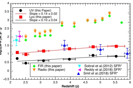
Figure 14.SFR evolution with redshift. Red squares: calculated using Lyαluminosities; black circles: calculated using rest frame UV magnitude; orange triangles: from 1.4 GHz radio stacking; green diamonds: FIR stacking. Results fromSmit et al. (2012), including those derived from Sobral et al. (2012a) and Reddy et al.(2008), are plotted for comparison. Radio and FIR values are upper limits from non-detections (detailed in Section6.2). We find that SFR increases with redshift across all tracers: Lyα, rest frame UV, FIR, and radio.

0.099_±0.004. This demonstrates that SFRLyαdiverges from

SFRUV, which is due to the presence of dust and a

vary-ing ionisation rate. Radio data provides upper limits on the SFR, and it is therefore in line with expectation that they form the ‘ceiling’ values in Figure14. As with Lyαand UV, SFR1.4GHz increases with redshift. No line of best fit was

plotted because theses results are from non-detections. FIR data are also upper limits, and combined with UV would roughly trace the SFR given by radio stacking, and therefore give the total SFR, as FIR traces obscured star formation and UV traces unobscured.

In Figure14, the errors on redshift, SFRLyαand SFRUV

are standard errors, calculated from the standard deviation.

If error bars cannot be seen on SFRLyα and SFRUV, it is

because they are contained within the points themselves.

The errors on the SFRFIR results were derived from

uncertainties on the calculated fFIRupper limits. These were

determined by fitting and integrating two black body curves – the best and least acceptable fits – to the flux density

upper limits (3 × noise from stacking) for each redshift.

The difference between the fFIR value obtained from each

integration was taken to be the error on the flux limit in each case. The fractional error in each case was equated to the fractional error for SFRFIRvalues to determine the SFR

uncertainty. As the SFRFIR are upper limits, lower limit

error bars were neglected. As such, only the positive error was plotted, effectively giving the absolute upper limit of

SFR. This is not visible on Figure 14 as the errors were

negligible compared to the scale of the plot.

The errors on the radio SFR values were calculated by equating the fractional errors of SFR1.4GHzand S1.4GHz. This

was done as, from Equation9 and Equation 10, it can be

seen that SFR1.4GHzis proportional to flux density S1.4GHz.

As with the FIR SFR results, only the positive errors were included on the Figure14, giving the true upper limits.

lo

g10

(S

F

R

D

[

M⊙

y

r

-1M

p

c

-3])

−4 −3 −2 −1 0

Redshift (z)

1.5 2 2.5 3 3.5 4 4.5 5 5.5 6

Lyα Slope = -0.11 ± 0.02

UV Slope = -0.3 ± 0.1

Gruppioni et al. (2013) Rowan-Robinson et al. (2016)

Figure 15.SFRD evolution with redshift. Green circles: calcu-lated using Lyαluminosities; blue squares: calculated using UV magnitudes; black diamonds:Gruppioni et al.(2013); red trian-gles:Rowan-Robinson et al.(2016). We find that SFRD decreases with increasing redshift.

Figure 15 shows that SFRD decreases with

in-creasing redshift in the range z _∼ 2.2 ₋ 5.5.

We find d

dzlog10(

SFRDLyα

Myr−1_Mpc−3) = −0.11 ± 0.02, and d

dzlog10(

SFRDUV

Myr−1_Mpc−3) =−0.3±0.1. In a similar fashion to

Figure14, SFRDLyαdiverges from SFRDUV, again thought

to be due to dust and the ionisation rate.

5 PROGENITOR ANALYSIS

When studying objects at high redshifts it is important to remember that the further away a galaxy is, the earlier in its evolutionary lifetime it appears. This means that, by looking at a wide range of redshifts, we can effectively watch the evo-lution of these young galaxies. In this section we attempt to study young LAE galaxies that will eventually evolve into

one of 3 types of z = 0 galaxies, these are dwarf, Milky

Way-like, and brightest cluster galaxies (BCGs). Their ear-lier forms are referred to as dwarf-like, Milky Way-like and cluster-like progenitor galaxies. In the study of the evolu-tionary path of these progenitors, and particularly those in the Milky Way-like category, we can learn much about the history of our own galaxy and those nearby to us.

5.1 Methodology

5.1.1 Identifying Progenitors using Luminosity

To find progenitors in the SC4K catalogue we used

Khosto-van et al.(2018) as reference, in which LAE dark matter

ha-los masses are related to their luminosities. The dark matter evolutionary track of present day galaxies with halo masses

∼1011−14M were plotted in their paper (in which dwarf

galaxies, Milky Way-type galaxies and BCGs are classified as

having_∼1011_M

halo mass Mhalo of dwarf-like, Milky Way-like and

cluster-like galaxy progenitors were found at redshifts matching our redshift slices. This data was then used in Equation 18, to produce average values for the Lyαluminosity of progenitor galaxies at these same redshifts. In the case of cluster-like progenitors, their dark matter halo masses are greater than 1013_M

so instead of using the range of the luminosity er-rors as limits for choosing our progenitors, Equation18was

used with the Mhalo= 1013Mand Mhalo= 1014Mlines

fromKhostovan et al.(2018) with the range of errors on the

luminosities produced as the extended range of luminosities for cluster-like progenitors.

log10(L(z)) = 1 2.08+0₋₀._.12₁₂

log10

Mhalo M

−12.19₋+0_0..06₀₆+log10(L?(z)) (18)

Where Equation 18is derived (under the condition L<L? as this is true for the majority of our Lyαluminosities, with the exception being 2< z <3.5, Mhalo∼1014 M, cluster-like progenitors, for which 2.08+0₋0..1212is replaced by 0.63+0−0..1212)

fromKhostovan et al.(2018). L(z) and Mhaloare the average

Lyαluminosity and dark matter halo mass of the progenitor

in question, and L?_{(z) is the Lyαcharacteristic line} lumi-nosity at redshiftz. These values were then used to isolate which galaxies in our data set would later evolve into dwarf-like, Milky Way-like and cluster-like galaxies. No dwarf-dwarf-like, a small number of Milky Way-like, and a much larger num-ber of cluster-like progenitors were found (see Table7). This is likely due to the selection bias present in high redshift detections as only the most massive of galaxies have lumi-nosities high enough to be observed at such great distances. Thus the progenitors of cluster-like galaxies will be more highly represented than Milky Way-like progenitors as they are more massive and luminous. The same applies to Milky Way-like versus dwarf-like progenitors. The resulting sets of Milky Way-like and cluster-like progenitors were used to calculate mean values per redshift of the galactic properties listed in Section 3.1.1, Section 3.1.2 and Section 3.1.3 for both sets, along with standard deviation errors. Addition-ally, when discussing progenitor results the lookback time is used in place of redshift in order to better represent the progenitor galaxy’s evolution with time.

5.1.2 Identifying Progenitors through SFR

To determine what SFR a galaxy with a specified mass needs in order to evolve into a galaxy with a mass similar to the Milky Way, we made the assumption that SFR is constant across cosmic time. With this assumption, we can easily in-tegrate SFR with respect to time to determine how much mass is added to a galaxy over time.

MMWP= MMW−[SFR×LBT] (19)

MMWP is the mass of the Milky Way progenitor galaxies,

MMWis the mass of the Milky Way, and LBT is the

Look-back Time. We use MMW= 6.43×1010MfromMcMillan

(2011).

Figure19shows what mass a galaxy should have at the

time we are observing them, for a given average SFR, in order to have a stellar mass equal to the Milky Way now.

5.2 Results

5.2.1 Progenitor Morphologies

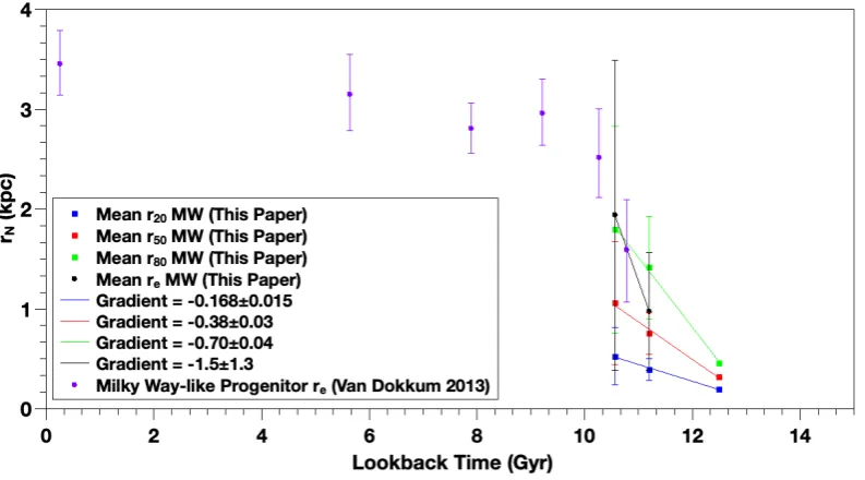
For the set of Milky Way-like progenitors it can be seen from Figure16that all measurements of the progenitor’s radii are increasing with age (increase inr20= 0.168±0.015 pcMyr−1,

increase in r50 = 0.38±0.03 pcMyr−1, increase in r80 =

0.70_±0.04 pcMyr−1 _{and tentative increase in r}

e = 1.5± 1.3 pcMyr−1) and, particularly forre, fit with results from the literature. As in Section4.1.2, the 50% to 80% light radii range is increasing faster than that of the 20% to 50% range, if slightly slower (_∼1.5 times faster, rather than_∼1.75 as

before). As Figure17shows, the Milky Way-like progenitors

have stellar masses which are increasing with age at a rate of 100.1±1.0 _M

Gyr−1. This data doesn’t fit as well as the

re data but it does within standard deviation error. The

progenitors’ S´ersic index values do not fit well with literature values, however it does still fall within the range of its large error bars. There is only one Milky Way-like progenitor data point for VC mean which is 0.9±1.1 which corresponds to a compact visual morphology, it does however have large errors due to a wide range of visual morphologies contained within this one mean.

Like those of the Milky Way-like progenitor radii, all measurements of cluster-like progenitor radii are increas-ing with age (increase in r20 = 0.08±0.02 pcMyr−1,

in-crease in r50 = 0.16±0.04 pcMyr−1, increase in r80 =

0.23_±0.11 pcMyr−1 _{and tentative increase in r}

e = 0.23± 0.16 pcMyr−1_{). Unlike in Section4.1.2and with the Milky}

Way-like progenitors, the 50% to 80% light radii range are increasing at roughly the same rate as the 20% to 50% range. The results for cluster-like progenitor radii fit with

the lowest results from Nelson et al. (2002), however, in

order to fit with the majority of the rest of the results

from Nelson et al. (2002), there would have to be a

sig-nificant increase in rate of increase of radii (from a rate of increase in re = 0.23±0.16 pcMyr−1 to a, post lookback time = 10.5, rate of increase of _∼4.5 pcMyr−1_{, so a rate}

∼ 20 times larger). Figure 18 shows that the cluster-like

progenitors appear to have a greater rate of stellar mass loss than that of the full SC4K set with a tentative decrease of 100.11±0.06_M

Gyr−1 which does not agree with data from

Stott et al.(2010). There are still large errors on the points

however, and they increase in size with age. The S´ersic in-dex values for this set of progenitors fit well with the lower

values ofn fromNelson et al.(2002) and would only need

a small increase in their rate ofn increase with time to fit with the majority of the rest of the values fromNelson et al.

(2002). However, they have very large error bars and have

a very wide spread across a the range 0< n <2.5. In the case of cluster-like galaxies there are more VC mean data points than for the Milky Way-like progenitors which shows almost no evolution with time (rate of VC mean decrease = 0.1_±0.3 Gy−1_).

5.2.2 Progenitor SFR

Figure 19shows that, for our sample, most early galaxies

must have an average SFR . 100.73 _M

yr−1 over their lifetimes in order to have a stellar mass similar to that of the Milky Way today. However, given that our average SFR = 101.103±0.005_M