The Bezier Control Points Method for Solving Delay
Differential Equation
Fateme Ghomanjani, Mohammad Hadi Farahi
Department of Applied Mathematics, Ferdowsi University of Mashhad, Mashhad, Iran Email: [email protected], [email protected]
Received December 19,2011; revised January 30, 2012; accepted February 9,2012
ABSTRACT
In this paper, Bezier surface form is used to find the approximate solution of delay differential equations (DDE’s). By using a recurrence relation and the traditional least square minimization method, the best control points of residual function can be found where those control points determine the approximate solution of DDE. Some examples are given to show efficiency of the proposed method.
Keywords: Bezier Control Points; Delay Differential Equation; Residual Function; Boundary Value Problem; Proportional Delays
1. Introduction
Delay differential equations are type of differential equa-tions where the time derivatives at the current time de-pend on the solution, and possibly its derivatives, at pre-vious times. A class of such equations, which involve derivatives with delays as well as the solution itself has been called neutral DDEs over the past century (see [1, 2]).
The basic theory concerning the stable factors and works on fundamental theory, e.g., existence and unique- ness of solutions, was presented in [1,2]. Since then, DDE have been extensively studied in recent decades and a great number of monographs have been published including significant works on dynamics of DDEs by Hale and Lunel [3], on stability by Niculescu [4], and so on. The interest in study of DDEs is caused by the fact that many processes have time-delays and have been models for better representations by systems of DDEs in science, engineering, economics, etc. Such systems, however, are still not feasible to actively analyze and con- trol precisely, thus, the study of systems of DDEs has actively been conducted over the recent decades (see [1, 2]).
In this paper, we show a novel strategy by using the Bezier curves to find the approximate solution for delay differential equations by Bezier curves. Other numerical methods for DDEs are available in (see [5-8]). In Section 2 delay differential equations will be introduced. Exam-ple of Time-Delay System will be stated in Section 3. In Section 4 delay differential equations with proportional delay will be introduced. Bezier curves and degree
eleva-tion will be stated in Seceleva-tions 5 and 6 respectively. In Section 7 solution of delay differential equation using Be- zier control points presented and aforementioned method will be implemented on it. In Section 8, solved numerical examples, showed the efficiency and reliability of the method. Finally, Section 9 will give a conclusion briefly.
2. Delay Differential Equations
Most delay differential equations that arise in population dynamics and epidemiology model intrinsically nonnega- tive quantities. Therefore it is important to establish that nonnegative initial data give rise to nonnegative solutions. Consider the following
,
,
u t f t u t u t h
, ,
(2.1) with a single delay h > 0. Assume that f t u y and
, ,
u t u y are continuous on R3. Let s
f R be given
and let :
s h s ,
R be continuous. We seek a so- lution u t
of (2.1) satisfying
,u t t s h t s
s t s
(2.2) and satisfying (2.1) on for some 0
u s .
Note that we must interpret as the right-hand de-rivative at s.
Now, we present a typical example of physical sys-tems that exhibit time-delay phenomena. The example selected in this section fit nicely into the model (2.1).
3. Example of Time-Delay System
systems is quite natural since there must be finite period of time following a decision for its effects to appear. In one model [9] of aggregate economy, we let Y t
be the income which can split into consumption C t
,in-vestment I t and autonomous expenditure. Thus
Y t C t I t E t
,C t cY t
(3.1) Define
(3.2) where c is a consumption coefficient. From (3.1) we get
1
I t E t c
Y t (3.3) It is assumed that there is finite interval of time be-tween ordering and delivery of capital equipment fol-lowing a decision to invest D t
.,
In terms of the stock of capital assets U t
we have
D t h
U t (3.4)
t
d .t hD
1
I t
h
D t
Y t
U t
(3.5) Economic rationale implies that is determined by the rate of saving (proportional to ) and by the capital stock . This means that
1
U t
,D t c Y t
0
(3.6)
where , 0 and ε is a trend factor. Combining (3.4) and (3.5), we obtain:
1
I t U
h t h U t
(3.7) By (3.3) and (3.7), we arrive at
1
1
Y t U t h h c
1
E t U t
c
(3.8)
Finally, it follows from (3.5), (3.6) and (3.8) that
U t U t U t h
h h
E t
1
0 ,
0,
m m
m k
k k
k
u t a t u p t
u t b t u p t f t
t
1
0 0 , 0,1, , 1.
m k
ik
k c u i i m
(3.9)
which expresses the formation of the rate of delivery of the new equipment. This is a typical functional differen-tial equation (FDE) of retarded type.
4. Delay Differential Equations with
Proportional Delay
In this paper, approximate analytical solutions with high accuracy can be obtained by carrying out in the Bezier control points method.
Consider the following neutral functional-differential equation with proportional delays (see [10-12]),
(4.1) with the initial conditions
(4.2)
a t and
Here, b t kk 0,1, , m1
are given analytical functions, and , pk, cik, i denote givenconstants with 0pk 1
k0,1, , m
.The existence and the uniqueness of the analytic solu-tion of the multi-pantograph equasolu-tion are proved in [13], the Dirichlet series solution is constructed, and the suffi-cient condition of the asymptotic stability for the analytic solution is obtained. It is proved that the θ-methods with a variable stepsize are asymptotically stable if 1 1.
2
1
0 ,
0,
m m
m
m k
k k
k
u t u t a t u p t b t u p t f t t
Some numerical examples are given to show the proper-ties of the θ-methods.
In order to apply the Bezier control points method, we rewrite Equation (4.1) as
Neutral functional-differential equations with propor-tional delays represent a particular class of delay differ-ential equation. Such functional-differdiffer-ential equations play an important role in the mathematical modeling of real world phenomena [14]. Obviously, most of these equa-tions cannot be solved exactly. It is therefore necessary to design efficient numerical methods to approximate their solutions. Ishiwata et al. used the rational approxi-mation method [15] and the collocation method [16] to compute numerical solutions of delay differential equa-tions with proportional delays. Hu et al. [17] applied lin-ear multistep methods to compute numerical solutions for neutral delay differential equations. Wang et al. obtained approximate solutions for neutral delay differential equa-tions by continuous Runge-Kutta methods [18] and one- leg θ-methods [13,19].
5. Bezier Curves
A Bezier curve of degree n can be defined as follows (see [19]):
,
0 , , ,
n i i n i
t a
C t P B t a b b a
(5.1)where ,
i n i
i n
n
t a t a b t
B
i
b a b a b a
are the Bern-
0 P 1 P 2 P 3 Pstein polynomials over the interval a b,
i
P
, 0,1 ,
1 n i.
t t
t
C t
. The Bezier coefficient is called the control point (see Figure 1). In particular
, 0 , n i i n ii i n
C t P B n B t t
i
(5.2)
If be a vector-valued polynomial, then C t
,
P P
is called a parametric Bezier curve. The control polygon of a Bezier curve comprise of the line segments i i1
. If is a scalar-valued polynomial, we call the function
0, 1
C t
1, ,
i n
y C t
1, , 1
P P
an explicit Bezier curve by
t C t,
(see [20,21]).6. Degree Elevation
Suppose we were designing with Bezier curve as de-scribed, and use a Bezier polygon of degree n to ap-proximate the desired given shape. Suppose the degree polygon dose not feat neatly the desired shape.
One way to proceed in such a situation is to increase the flexibility of the polygon by adding another vertex (control point) to it. As a first step, one might want to add another vertex, yet leave the desired curve of the shape unchanged, this corresponds to raising the degree of the Bezier curve by one (see Figure 2). Therefore, we are looking for a curve with control vertices 0 n1
, ,
P P
that describes the same curve of the shape as the original polygon 0 n (see [21-25] for more details).
We rewrite our given Bezier curve as
1 1, 1 1 1 1 n i n ii i n
P t
t
P B t
1 , 0 0 0 1 0 1 1 ! 1 11 ! 1 !
1 ! 1
1 ( 1)! !
1 1 n i i n i i n n
i i n i
i
i i
C t t C t tC t
n
n i
n i n i
n i
Pt
n i n i
n iPB t i
n t n
The upper index of the first sum may be extended to n
+ 1, since the corresponding term is zero. The summation indices of the second sum may be shifted to index 1 and
n + 1, but one may choose the lower index zero since only a zero term is added. Thus we have
, 1
, 1
1 , 1 1
1
n
i i n
i i n
t n iPB t
P B t
1 1 0 1 0 1 0 1 n i i i n i n i
C t P B
n i n
[image:3.595.312.535.83.211.2]
(6.1) Combining both sums and computing coefficients [image:3.595.307.540.243.461.2]Figure 1. A degree three Bezier curve and its control poly-gon.
Figure 2. Repeated degree elevation.
yields: 1
1 1 , 0,1, , 1,
1 1
i i i
i i
P P P i n
n n
1 P (6.2)
where i is the control point of the Bezier curve C t
when it is elevated to degree n + 1. Now, the new control polygon consists of n + 2 control points.7. Solution of Delay Differential Equation
Using Bezier Control Points
Consider the following boundary value problem
0 1 1 0 , , , , , 0,d 0 d 1
, , 0,1, , 1,
d d m m m m m k k k k i i i i i i
L u t u p t u p t u p t u t u t a t u p t
b t u p t f t t
u u i m t t
(7.1) where L is differential operator with proportional delay,
f t is also a polynomial in t, and 0 pk 1 (k = 0, 1, ··· , m) [26].
[image:3.595.73.272.461.571.2]the Bezier form is easier to symbolically carry out the operations of multiplication, comparison and degree ele-vation than B-spline form. We choose the sum of squares of the Bezier control points of the residual to be the measure quantity. Minimizing this quantity gives the ap- proximate solution. So, the obvious spotlight is in the following, if the minimizing of the quantity is zero, so the residual function is zero, which implies that the solu-tion is the exact solusolu-tion. We call this approach the con- trol-point-based method. The detailed steps of the method are as follows (see [24]):
Step 1. Choose a degree n and symbolically express the solution u t
in the degree n n m
Bezier form
u u t
0 ,
,n i i n i a B t
0, , ,1 n
a a a
(7.2) where the control points are to be de-termined.
Step 2. Substituting the approximate solution
u u t
into the differential Equation (7.1), we gain the re-sidual function
, p tm
f t
.
0 deg , eg .n b t
f t
R t
, 0 , k i i k i b B t, , ,
b b b a
i
0 1
, , ,
R t L u t u p t u p t u
This is a polynomial in t with degree ≤k, where
1 1max deg ,
1 deg , ,
1 deg m ,d
k n m a t n b t n m b t
So the residual function can be expressed in Bezier form as well,
R R t
(7.3) where the control points 0 1 k are linearfunc-tions in the unknowns i. These functions are
de-rived using the operations of multiplication, degree elevation and differentiation for Bezier form.
Step 3. Construct the objective function 2
0 .
k i
F
bThen F is also a function of 0, , ,1 n.
Step 4. Solve the constrained optimization problem:
a a a
2
0 1
0
min , , ,
d 0 d 1
, , d d k i n i i i i i i i
F b a a
u u
t t
,0,1, , 1,
a
i m
(7.4) by some optimization techniques, such as Lagrange multipliers method, we can be used to solve (7.4). Step 5. Substituting the minimum solution back into
(7.2) arrives at the approximate solution to the dif-ferential equation.
8. Numerical Examples
In this part, we used the mentioned control-point-based
method on Bezier control points to solve DDE’s and system of DDE’s.
Example 8.1. As a practical example, we consider Evens and Raslan [6] the following pantograph delay equation:
1exp 1 , 0 1, 0 1
2 2 2 2
t t
u t u u t t u
.
The exact solution is u t
exp
t . Now we try to find a degree two approximate solution. Let
0 0,2
1 1,2
2 2,2
u t a B t a B t a B t .
Substituting it into the above delay differential equation gives R t
as:
2 21 1 2 2
3 4 4 4 2
1 1 2 1
0 0,4 1 1,4 2 2,4
3 3,4 4 4,4
1exp 1
2 2 2 2
13 11 7 5
3 2 2
4 2 16 8
1 1 1 1
16 16 32 64
,
t t
R t u t u u t
t a a t a t t a t
a t t a t a t a t
b B t b B t b B t
b B t b B t
4 3 0,4 1,4 22 3 4
2,4 3,4 4,4
1 , 4 1 ,
6 1 , 4 1 , .
B t t B t t t
B t t t B t t t B t t
where
Then construct the function
2 2
0 1 2 1 1 2
2 2
2 1 2 1
193 141 5 1
, , 2
64 64 8 2
75 51 103 5 7 39
64 64 64 4 32 16 .
F a a a a a a
a a a a
0, ,1 2
F
Minimizing a a a with u
0 a0 1 and u(1) = a2 = exp(1). We obtain
1
174691 189589exp 1 488905 488905
a .
Thus the approximate solution is
1 0.822827885 0.89545394332u t t t .
In Figure 3 compare approximated and exact value of
u t . Figure 4 shows the residual function.
Example 8.2. Consider the previous example with de-gree raising in Bezier control points.
Let
0 0,8 1 1,8 2 2,8
3 3,8 4 4,8 5 5,8
6 6,8 7 7,8 8 8,8 .
u t a B t a B t a B t
a B t a B t a B t
a B t a B t a B t
Figure 3. Approximate and exact solution of u(t) for
Exam-ple 8.1. Figure 4. Residual function for Example 8.1.
R t as: Substituting it into the delay differential equation leads to
8 63 3
7
1 1
4 5
2 2
1799 71715
64 32
5895 15239 18
64 32
48293 5607 1
16 2
R t a t a t
a t a t
a t a t
7 8 7 8 8 6
3 6 6 7 5 5
6 5 4 3 2 8 3
1 1 1 1 1 2
3577 16135 3577 10087
9 588 4
256 64 128 8
389 12355 4845 538 521 7091
16 8 4 128 4
97
a t a t a t a t a t a t
a t a t a t a t a t a t
7 5 4 2 5 3
2 6 4 2 5 3
4 7 6 5 4 7
5 8 6 1 3 3 4
6 7 2
2
19 22995 1043 8295 2303
168
64 16 2 8 2
12999 58317
8 118 2947 700
32 16
88739 385 2953
31
64 32 16
a t a t a t a t a t a t
a t a t a t a t a t a t a t
a t t t
8 7
8 7
6 7
4 5
257 2177 280
512 32
277935 34055
128 64
a t a t
a t a t
3 8 4 5
8 6 5 9 10 8 9 9
4 4 8 2
9 9 9 10 10
5 7 3 4 8 2 1
263 2527 6279
0
512 8 32
967 85225 3 1 1 7
8 35
28 32 1024 4096 1024 128
1 21 35 1 7 1
256 256 512 4096 1024 512
t t t t
t a t t t a t a t a t
a t a t a t a t a t a t
1 2
9 6 9
1 7
247 3619 8
4 256 1
5 7
56
256 256
t a a t
a t a t a t
10 10
5 7
0 0,10 1 1,10 2 2,10
7 1
512a t 512a t 1024
b B t b B t b B
10
10 10 10 3 2
6 3 4 2 4 3
3 3,10 4 4,10 5 5,10 6 6,10
7 7,10 8 8,10 9 9,10 10 10,10
7 7 35
56 280 168
512 2048
.
a t a t a t a t a t a t t b B t b B t b B t b B t b B t b B t b B t b B t
Then construct the function
0, , ,1 2 3 4, , , ,5 6 7 8
F a a a a a a a a a
0 0 1u a
and minimizing F with
1 1.125570325,
a a21.268969764,
3 1.433189859,
a 4
5 1.838975663,
a
1.621779319,
a
a6
7 2.380493436.
a
2.089850744, and
and u(1) = a8 =
exp(1). We obtain
[image:5.595.88.505.381.646.2]
8 7
6
2
8
1 9.004562600 1
35.53115339 1 80.2586 113.5245523 1 102.982 58.51582083 1 19.043947 2.718281828 .
u t t t t
t t t t t t t
5
2 3
4 3
4 5
6 7
3210 1 6371 1
49 1
t t t t
t t
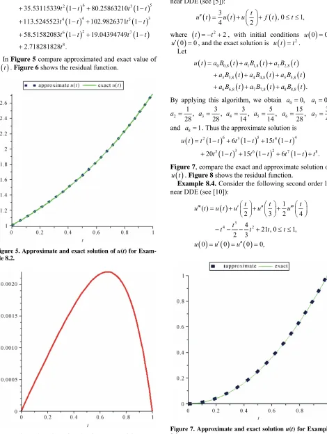
In Figure 5 compare approximated and exact value of
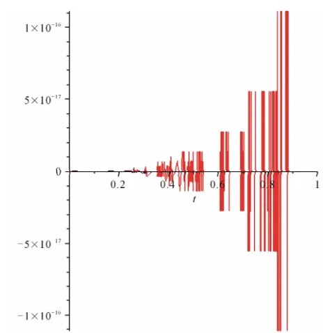
[image:6.595.303.537.87.328.2]u t . Figure 6 shows the residual function.
Figure 5. Approximate and exact solution of u(t) for Exam-ple 8.2.
Figure 6. Residual function for Example 8.2.
Example 8.3. Consider the following second order li-near DDE (see [5]):
3
, 0 1,4 2
t
u t u t u f t t
t t2 2 u
0 0,where , with initial conditions
0 0u , and the exact solution is u t
t2. Let
0 0,8 1 1,8 2 2,8
3 3,8 4 4,8 5 5,8
6 6,8 7 7,8 8 8,8 .
u t a B t a B t a B t a B t a B t a B t a B t a B t a B t
0 0,
a a1 0, By applying this algorithm, we obtain
2
1 28
a , 3
3 28
a , 4
3 14
a , 5
5 14
a , 6
15 28
a , 7
3 4
a
8 1
a . Thus the approximate solution is and
6 5 4
2 3 4
3 2
5 6 7 8
1 6 1 15 1
20 1 15 1 6 1 .
u t t t t t t t
t t t t t t t
[image:6.595.63.533.102.727.2]
Figure 7, compare the exact and approximate solution of
u t
. Figure 8 shows the residual function.
Example 8.4. Consider the following second order li-near DDE (see [10]):
3
4 2
1 ( )
2 3 2 4
4
21 , 0 1,
2 3
0 0 0 0,
t t t
u t u t u u u
t
t t t t
u u u
[image:6.595.58.288.214.452.2]
Figure 7. Approximate and exact solution u(t) for Example 8.3.
[image:6.595.308.538.394.708.2]Figure 8. Residual function for Example 8.3.
where the exact solution is u t
t4
2 2,8
5 5,8
8 8,8 .
a B t t a B t t a B t
0,
a1 0,
. Let
0 0,8 1 1,8
3 3,8 4 4,8
6 6,8 7 7,8
u t a B t a B t a B t a B a B t a B
By applying this algorithm, we obtain a0
2
a 0, a30, 4
1 , 70
a 5 1 , 14
a a6 3 ,
14 7
1 2
a and a81. Thus the approximate solution is
4 3
6 7 8
1
.
1 1
t
t t t
u t
1 , 0 1, 1, 0,
t t
y
1
4 5
2
1 4
6 4
u t t t t
t t
Figure 9, compare the exact and approximate solution of . Figure 10 shows the residual function.
Example 8.5. In this example the following first order linear DDE’s is considered (see [13]):
u t u t
u t
Since
0 0 and y
0 y
1 , y t
has a jump at t = 0. The second derivative y t
y t
1 ,
y t
and therefore it has a jump at t = 1.
Now we try to find an approximate solution. Let
t a B3 3,3
t0 1
a
3127 a30
0 0,3 1 1,3 2 2,3
u t a B t a B t a B .
By applying this algorithm, we acquire ,
, , . Thus
1
a 0.7806290653 a20.335917
[image:7.595.304.539.82.314.2]Figure 9. Approximate and exact solution u(t) for Example 8.4.
Figure 10. Residual function for Example 8.4.
the approximate solution is
3 2
2
1 2.341887196 1 1.007751938 1 .
u t t t t
t t
u t
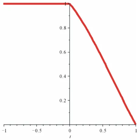
Figure 11 shows the approximate value of .
9. Conclusion
[image:7.595.52.541.88.551.2] [image:7.595.306.538.346.585.2]Figure 11. Approximate u(t) for Example 8.5.
the rough solution is expressed in Bezier form, then the residual function is minimized to find the best approxi-mate solution. Some examples are given to verify the reliability and efficiency of the proposed method.
REFERENCES
[1] G. Adomian and R. Rach, “Nonlinear Stochastic Differ- ential Delay Equation,” Journal of Mathematical Analysis and Applications, Vol. 91, No. 1, 1983, pp. 94-101. doi:10.1016/0022-247X(83)90094-X
[2] F. M. Asl and A. G. Ulsoy, “Analysis of a System of Lin- ear Delay Differential Equations,” Journal of Dynamic Systems, Measurement and Control, Vol. 125, No. 2, 2003, pp. 215-223. doi:10.1115/1.1568121
[3] J. K. Hale and S. M. V. Lunel, “Introduction to Func- tional Differential Equations,” Springer-Verlag, Berlin, 1993.
[4] S. I. Niculescu, “Delay Effects on Stability: A Robust Control Approach,” Springer, Berlin, 2001.
[5] A. K. Alomari, M. S. M. Noorani and R. Nazar, “Solution of Delay Differential Equation by Means of Homotopy Analysis Method,” Acta Applicandae Mathematicae, Vol. 108, No. 2, 2009, pp. 395-412.
doi:10.1007/s10440-008-9318-z
[6] D. J. Evans and K. R. Raslan, “The Adomian Decomposi-tion Method for Solving Delay Differential EquaDecomposi-tion,” International Journal of Computer Mathematics, Vol. 82, No. 1, 2005, pp. 49-54.
doi:10.1080/00207160412331286815
[7] S. J. Liao, “Series Solutions of Unsteady Boundary-Layer Flows over Plate,” Mathematical Analysis and Applica- tions, Vol. 117, No. 3, 2006, pp. 239-263.
doi:10.1111/j.1467-9590.2006.00354.x
[8] F. Shakeri and M. Dehghan, “Solution of Delay Diffren-
tial Equation via a Homotopy Perturbation Method,” Ma- thematical and Computer Modelling, Vol. 48, No. 3-4, 2008, pp. 486-498. doi:10.1016/j.mcm.2007.09.016 [9] H. Gorecki, S. Fuksa, P. Grabowski and A. Korytowski,
“Analysis and Synthesis of Time Delay Systems,” John Wiley and Sons, New York, 1989.
[10] X. Chen and L. Wang, “The Variational Iteration Method for Solving a Neutral Functional-Differential Equation with Proportional Delays,” Computers and Mathematics with Applications, Vol. 59, No. 8, 2010, pp. 2696-2702. doi:10.1016/j.camwa.2010.01.037
[11] Z. Fan, M. Liu and W. Cao, “Existence and Uniqueness of the Solutions and Convergence of Semi-Implicit Euler Methods for Stochastic Pantograph Equations,” Mathe- matical Analysis and Applications, Vol. 325, No. 2, 2007, pp. 1142-1159. doi:10.1016/j.jmaa.2006.02.063
[12] R. Bellman and K. L. Cooke, “Differential-Difference Equations,” Academic Press, London, 1963.
[13] W. Wang, T. Qin and S. Li, “Stability of One-Leg θ- Methods for Nonlinear Neutral Differential Equations with Proportional Delay,” Applied Mathematics and Com- putation, Vol. 213, No. 1, 2009, pp. 177-183.
doi:10.1016/j.amc.2009.03.010
[14] A. Bellen and M. Zennaro, “A Reviw of DDE Meth- ods,” In: G. H. Golub, C. H. Schwab, W. A. Light and E. Suli, Eds., Numerical Methods for Delay Differential Equations, Numerical Mathematics and Scientific Com-putation, Clarendon Press, New York, 2003, pp. 36-60. [15] E. Ishiwata and Y. Muroya, “Rational Approximation
Method for Delay Differential Equations with Propor- tional Delay,” Applied Mathematics and Computation, Vol. 187, No. 2, 2007, pp. 741-747.
doi:10.1016/j.amc.2006.08.086
[16] E. Ishiwata, Y. Muroya and H. Brunner, “A Super-At- tainable Order in Collocation Methods for Differential Equations with Proportional Delay,” Applied Mathemat- ics and Computation, Vol. 198, No. 1, 2008, pp. 227-236. doi:10.1016/j.amc.2007.08.078
[17] P. Hu, C. Huang and S. Wu, “Asymptotic Stability of Linear Multistep Methods for Nonlinear Neutral Delay Differential Equations,” Applied Mathematics and Com- putation, Vol. 211, No. 1, 2009, pp. 95-101.
doi:10.1016/j.amc.2009.01.028
[18] W. Wang, Y. Zhang and S. Li, “Stability of Continuous Runge-Kutta-Type Methods for Nonlinear Neutral Delay- Differential Equations,” Applied Mathematical Modelling, Vol. 33, No. 8, 2009, pp. 3319-3329.
doi:10.1016/j.apm.2008.10.038
[19] W. Wang and S. Li, “On the One-Leg θ-Methods for Solving Nonlinear Neutral Functional Differential Equa- tions,” Applied Mathematics and Computation, Vol. 193, No. 1, 2007, pp. 285-301. doi:10.1016/j.amc.2007.03.064 [20] G. Farin, “Curves and Surfaces for CAGO: A Practical
Guide,” Morgan Kaufmann, Waltham, 2001.
[21] G. Farin, “Curves and Surfaces for Computer-Aided Geo- metric Design: A Practical Guide,” 4th Edition, Academic Press, London, 1997.
[22] S. Mann, “A Blossoming Development of Spliness,” Mor-
gan Claypool, San Rafael, 2004.
[23] S. Biswa and B. Lovell, “Bezier and Splines in Image Processing and Machine Vision,” Springer-Verlag, Berlin, 2008.
[24] J. Zheng, T. Sedberg and R. Johansons, “Least Squares Methods for Solving Differential Equation Using Bezier Control Points,” Applied Numerical Mathematics, Vol. 48, No. 2, 2004, pp. 137-152.
doi:10.1016/j.apnum.2002.01.001
[25] B. Egerstedt and F. Martin, “A Note on the Connection between Bezier Curves and Linear Optimal Control,” IEEE Transactions on Automatic Control, Vol. 49, No. 10, 2004, pp. 1728-1731. doi:10.1109/TAC.2004.835393