Static Analysis and Code Complexity Metrics as Early Indicators of Software Defects

http://www.scirp.org/journal/jsea ISSN Online: 1945-3124

ISSN Print: 1945-3116

DOI: 10.4236/jsea.2018.114010 Apr. 11, 2018 153 Journal of Software Engineering and Applications

Static Analysis and Code Complexity Metrics as

Early Indicators of Software Defects

Safa Omri

, Pascal Montag

, Carsten Sinz

1_{Daimler AG, Boeblingen, Germany}

2_{Karlsruhe Institute of Technology, Karlsruhe, Germany}

Abstract

Software is an important part of automotive product development, and it is commonly known that software quality assurance consumes considerable ef-fort in safety-critical embedded software development. Increasing the effec-tiveness and efficiency of this effort thus becomes more and more important. Identifying problematic code areas which are most likely to fail and therefore require most of the quality assurance attention is required. This article presents an exploratory study investigating whether the faults detected by static analy-sis tools combined with code complexity metrics can be used as software qual-ity indicators and to build pre-release fault prediction models. The combina-tion of code complexity metrics with static analysis fault density was used to predict the pre-release fault density with an accuracy of 78.3%. This combina-tion was also used to separate high and low quality components with a classi-fication accuracy of 79%.

Keywords

Static Analysis Tools, Complexity Metrics, Software Quality Assurance, Statistical Methods, Fault Proneness

1. Introduction

Software quality assurance is overall the most expensive activity in safety-critical embedded software development [1] [2]. Increasing the effectiveness and effi-ciency of software quality assurance is more and more important given the size, complexity, time and cost pressures in automotive development projects. Therefore, in order to increase the effectiveness and efficiency of software quali-ty assurance tasks, we need to identify problematic code areas most likely to contain program faults and focus the quality assurance tasks on such code areas.

How to cite this paper: Omri, S., Montag, P. and Sinz, C. (2018) Static Analysis and Code Complexity Metrics as Early Indica-tors of Software Defects. Journal of Soft-ware Engineering and Applications, 11, 153-166.

https://doi.org/10.4236/jsea.2018.114010

Received: January 11, 2018 Accepted: April 8, 2018 Published: April 11, 2018

Copyright © 2018 by authors and Scientific Research Publishing Inc. This work is licensed under the Creative Commons Attribution International License (CC BY 4.0).

DOI: 10.4236/jsea.2018.114010 154 Journal of Software Engineering and Applications Obtaining early estimates of fault-proneness helps making decisions on testing, code inspections and design rework, to financially plan possible delayed releases, and affordably guide corrective actions to the quality of the software [3].

One source to identify fault-prone code components can be their failure his-tory, which can be obtained from bug databases; a software component likely to fail in the past is likely to do so in the future [4]. However, in order to get accu-rate predictions, a long failure history is required. Such a long failure history is usually not available, moreover maintaining long failure histories is usually avoided altogether [4].

A second source to estimate fault-proneness of software components is the program code itself. Static code analysis and code complexity metrics have been shown to correlate with fault density in a number of case studies [5][6][7][8]. Static analysis evaluates software programs at compile time by exploring all possible execution paths [9] [10]. Static analysis tools can detect low-level pro-gramming faults such as potential security violations, run-time errors and logical inconsistencies [11]. Code complexity metrics have been proposed in different case studies to assess software quality [1][4][12].

In this article, we apply a combined approach to create accurate fault predic-tors. Our process can be summarized in the following three steps:

1) Data Preparation: the data required to build our fault predictors are: a) Static analysis faults: we execute static code analysis on each component. We define the static analysis fault density of a software component as the num-ber of faults found by static analysis tools, after reviewing and eliminating false positives, per KLOC (thousand lines of code).

b) Pre-release faults: we mine the archives of several major software systems at Daimler and map their pre-release faults (faults detected during development) back to its individual components. We define the pre-release fault density of a software component as the number of faults per KLOC found by other methods (e.g. testing) before the release of the component.

c) Code complexity metrics: we compute several code complexity metrics for each of the components.

2) Model Training: we train statistical models to learn the pre-release fault densities based on both a) static analysis faults densities, and b) code complexity metrics. In order, to overcome the issue of multicollinearity associated with combining several metrics as input variables of the statistical models, we apply the standard statistical principal component analysis (PCA) technique on the static analysis fault densities and the code complexity metrics.

3) Model Prediction: the trained statistical models are used to a) predict pre-release fault densities of software components (Regression) and, b) discrimi-nate fault-prone software components from the not fault-prone software com-ponents (Classification).

DOI: 10.4236/jsea.2018.114010 155 Journal of Software Engineering and Applications that is: Is combining static analysis tools with code complexity metrics a leading indicator of faulty code? The hypotheses that we want to confirm in this article are:

1) static analysis fault density combined with code complexity metrics can be used as an early indicator of pre-release fault density;

2) static analysis fault density combined with code complexity metrics can be used to predict pre-release fault density at statistically significant levels;

3) static analysis fault density combined with code complexity metrics can be used to discriminate between fault-prone and not fault-prone components.

The organization of the article is as follows. After discussing the state of the art in Section 2, we describe the design of our case study in Section 3. Our results are reported and discussed in Section 4. Section 5 concludes and discusses future work.

2. Related Work

2.1. Failures and Faults

In this work, we use the term fault to refer to an error in the source code. We re-fer to an observable error at program run-time as failure. We assume that, every failure can be traced back to a fault, but a fault does not necessarily result in a failure.

Faults which have been identified before a software release, typically during software testing, are referred to as pre-release faults. If faults are identified after a software release as a result of failures in the field (by the customer), then such faults are referred to as post-release faults. The focus of this work is on pre-release faults to obtain an early estimate of software component’s fault-proneness in order to guide software quality assurance towards inspecting and testing the compo-nents most likely to contain faults.

Fault-proneness is defined as the probability of the presence of faults in the software [13]. Such probability is estimated based on previously detected faults using techniques such as software testing. The research on fault-proneness has focused on 1) the definition of code complexity and testing thoroughness me-trics, and 2) the definition and experimentation of models relating metrics with fault-proneness.

2.2. Code Metrics

Software complexity metrics were initially suggested by Chidamber and Kemerer [14]. Basili et al.[15], and Briand et al.[5] were among the first to use such me-trics to validate and evaluate fault-proneness. Subramanyam and Krishnan [7], and Tang et al.[8] showed that these metrics can be used as early indicators of external software quality.

DOI: 10.4236/jsea.2018.114010 156 Journal of Software Engineering and Applications correlates with post-release faults, 2) there is no single set of metrics that fits all software projects, 3) predictors obtained from complexity metrics are good es-timates of post-release defects, and 4) such predictors are accurate only when obtained from the same or similar software projects. Our work builds on the study of Nagappan et al. [4], and focuses on pre-release faults while taking into consideration not only the code complexity metrics but also the faults detected by static analysis tools to build accurate pre-release fault predictors.

2.3. Statistical Techniques

A number of statistical techniques have been used to analyze software quality. Khoshgoftaar et al. [16], and Larus et al. [17] used multiple linear regression analyses to model the software quality as a function of software metrics. The coefficient of determination, R2_{, is usually used to quantify how much variability}

in the software quality can be explained by a regression model. A major difficul-ty when using regression models to combine several metrics is the issue of mul-ticollinearity among the metrics, which is explained by the existence of in-ter-correlations between the metrics. Multicollinearity can lead to an overesti-mation of the regression estimate. For example, high cyclomatic complexity usually correlates with a high amount of code lines [4].

One approach to overcome multicollinearity is applying Principal Component Analysis (PCA) [18] [19] on the metrics before applying regression modeling. Using PCA, a subset of uncorrelated linear combinations of metrics, which ac-count for the maximum possible variance, is selected for use in regression mod-els. Denaro et al.[13] used PCA on a study that considered 38 software metrics for the open source projects Apache 1.3 and 2.0 to select a subset of nine prin-cipal components which explained 95% of the total data variance. Nagappan et al.[4] used PCA to select a subset of five principal components out of 18 com-plexity metrics that account for 96% of the total variance in one of the studied commercial projects.

2.4. Static Analysis

DOI: 10.4236/jsea.2018.114010 157 Journal of Software Engineering and Applications Nagappan et al.[20] showed at Nortel Networks on an 800 KLOC commercial software system, that automatic inspection faults detected by static analysis tools were a statistically significant indicator of field failures and is effective to classify fault-prone components. Nagappan et al.[21] applied static analysis at Microsoft on a 22 MLOC commercial system and showed that the faults found by static analysis tools were a statistically significant predictor of pre-release faults and can be used to discriminate between fault-prone and non fault-prone compo-nents. Again, our approach does not only make use of the faults detected by static analysis, but also uses code complexity metrics; it goes beyond the works of Na-gappan et al. by not only using the faults detected by static analysis tools as an indicator of pre-release faults, but also combines these faults with code complex-ity metrics in a mathematical model which delivers a more accurate predictor and classifier of pre-release faults. It is important to note that the focus of our work as well as the related works [20][21] is on the application of non-verifying static analysis tools. The study of the impact of using verifying static analysis tools on the prediction accuracy of pre-release fault densities goes beyond the scope of this work and is planned as a future work.

3. Study Design

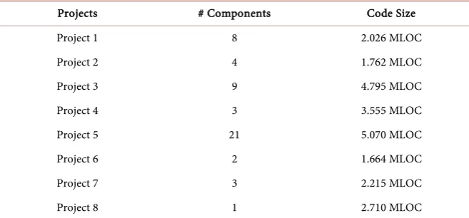
The goal of this article is to come up with fault predictors that evaluate our hy-potheses. Our experiments were carried out using eight software projects of an automotive head unit control system (Audio, Navigation, Phone, etc.). In the remainder of the article, we will be referring to these eight projects as Project 1 to 8. For reasons of confidentiality, we cannot disclose which number stands for which project. Each project, in turn, is composed of a set of components. The total number of components is 54. These components have a collective size of 23.797 MLOC (million LOCs without comments and spaces). All components use the object oriented language C++. Table 1 presents a high level outline of each project.

3.1. Faults Data

Daimler systematically records all problems that occur during the entire product life cycle. In this work, we are interested in pre-release faults, that is faults that have been detected before the initial release. For each component of the eight projects (Project 1 to Project 8 from Table 1), we extracted from an internal fault database all bugs detected for the latest release. The fault database is conti-nuously updated from testing teams, integration teams, external teams or third party testers. Such faults do not include problems submitted by customers in the field which are only found in post-release scenarios. The faults extracted from the fault database are then used to compute the pre-release fault density.

DOI: 10.4236/jsea.2018.114010 158 Journal of Software Engineering and Applications

Table 1. Software projects researched.

Projects # Components Code Size

Project 1 8 2.026 MLOC

Project 2 4 1.762 MLOC

Project 3 9 4.795 MLOC

Project 4 3 3.555 MLOC

Project 5 21 5.070 MLOC

Project 6 2 1.664 MLOC

Project 7 3 2.215 MLOC

Project 8 1 2.710 MLOC

3.2. Metrics Data

For each of the components, we compute a number of code metrics, as described in Table 2. We limit our study on the metrics commonly used and selected over a long period of time by the software quality assurance team at Daimler.

4. Case Study

The case study below details the experiments we executed to validate our hypo-theses. Table 3 defines abbreviations used in this section.

4.1. Correlation Analysis

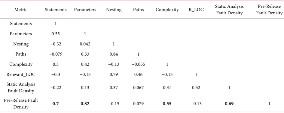
In order to investigate the possible correlations between the pre-release fault density and the code complexity metrics as well as the static analysis fault den-sity, we applied a robust correlation technique, Spearman rank correlation. Spearman rank correlation has the advantage over other correlation techniques such as Pearson correlation to detect also non-linear correlations between ele-ments.

Table 4 summarizes the correlation results. It shows a statistically significant positive correlation between the static analysis fault density and the pre-release fault density. It also shows a statistically significant positive correlation between the pre-release fault density and some of the code complexity metrics. The cor-relations between the code complexity metrics (row 1 to row 6), as well as be-tween the code complexity metrics and the static analysis fault density (row 7), are an early indicator of the existence of the multicollinearity problem when us-ing both code complexity metrics and static analysis fault density as input para-meters of statistical prediction models.

In this work we assume statistical significance at 99% confidence. Further-more, all metrics are normalized before computing the correlations.

4.2. Predictive Analysis

DOI: 10.4236/jsea.2018.114010 159 Journal of Software Engineering and Applications

Table 2. Metrics used for the study.

Metric Description

Statements # statements in a method

Parameters # function parameters in a method Nesting # nesting levels in a method

Paths # non-cyclic paths in a method

Complexity cyclomatic complexity of a method

Relevant_LOC # relevant LOCs of code without comments, blanks, expansions, etc.

Table 3. Nomenclature.

Abbreviations Description

PCA Principal component analysis (PCA) is a standard statistical procedure to convert a set of possibly correlated _{variables into a (typically smaller) set of linearly uncorrelated variables by using a coordinate transformation.}

R2 R squared: coefficient of determination, measures the variance in the predicted variable that is accounted by the

regression built using the predictors (code metrics combined with static analysis fault density).

MSE Mean squared error (MSE) is a measure of the unbiased error estimate of the error variance.

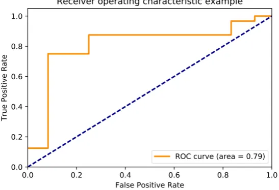
ROC curve Receiver operating characteristic (ROC) curve, is a popular measure for evaluating classifier performance. The ROC _{curve is created by plotting the true positive rate against the false positive rate at various threshold settings.}

AUC Area under curve (AUC) equals the probability that the classifier predicts a randomly chosen true positive higher than a randomly chosen false negative. The larger the AUC, the more accurate is the classification model.

Table 4. Correlation results of pre-release fault density with code metrics and static analysis fault density.

Metric Statements Parameters Nesting Paths Complexity R_LOC Static Analysis _{Fault Density Fault Density} Pre-Release

Statements 1

Parameters 0.55 1

Nesting −0.32 0,042 1

Paths −0.079 0.33 0.84 1

Complexity 0.3 0.42 −0.13 −0.055 1

Relevant_LOC −0.3 −0.13 0.79 0.46 −0.13 1 Static Analysis

Fault Density −0.22 0.13 0.37 0.067 0.31 0.52 1 Pre-Release Fault

Density 0.7 0.82 −0.15 0.079 0.55 −0.13 0.69 1

DOI: 10.4236/jsea.2018.114010 160 Journal of Software Engineering and Applications problem of multicollinearity between the independent variables (see Table 4 where correlations between code metrics have been identified), we used the standard statistical principal component analysis (PCA) technique. Multicolli-nearity might lead to an inflated variance in the estimation of the dependent va-riable, that is the pre-release fault density.

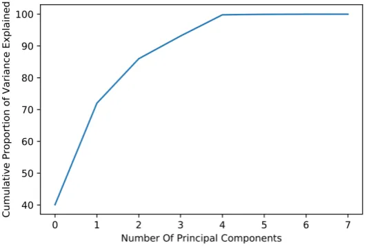
We extracted the principal components out of the 7 independent variables which include the six complexity metrics and the static analysis fault density. Figure 1 shows that 4 principal components result in variance close to 98%. Therefore, in this study, we selected the number of principal components as 4, which we used to model our prediction model. We split our data into two parts: 1) train data which accounts for 70% of the available data, and 2) test data representing the remaining 30%. We first transform both train and test data to 4 components which explained 98% of the total data variance using PCA. Then, we fit several models to the code complexity data, and the static analysis fault density separately as predictors and the pre-release fault density as the depen-dent variable. We then combined both code metrics and static analysis fault density as predictors for the pre-release fault density. The models we tested in-clude linear, exponential, polynomial regression models as well as support vector regressions and random forest. As a measure of the regression fits, we compute R2_{. R}2 _{measures the variance in the predicted variable that is accounted by the}

regression built using the predictors. As a measure of the unbiased error esti-mate of the error variance, we use the mean squared error (MSE).

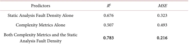
Table 5 shows that when using both the complexity metrics and the static analysis fault density as predictors, we obtain the best fit using the random forest model; the R2 _{value increases to 0.783 and the MSE decreases to 0.216.}

There-fore, we conclude that it is more beneficial to combine both code metrics and static analysis to explain pre-release faults. We do not present the regression eq-uations to protect proprietary data. The validation of the model goodness is re-peated 10 times using the 10-fold cross validation technique.

DOI: 10.4236/jsea.2018.114010 161 Journal of Software Engineering and Applications

Table 5. Regression fits.

Predictors R2 _MSE

Static Analysis Fault Density Alone 0.676 0.323 Complexity Metrics Alone 0.507 0.493 Both Complexity Metrics and the Static

Analysis Fault Density 0.783 0.216

In order to address the fact that the above results are not by chance we re-peated the data split (train: 70% and test: 30% of the data) as well as the model fitting several times. To quantify the sensitivity of the results we applied the Spearman rank correlation between the predicted and the actual pre-release fault densities. Table 6 reports the correlations as well as the accuracy (R2_{) of the}

pre-diction when applied on three random splits of the data. The Spearman correla-tion shows a strong positive correlacorrela-tion always stronger when both complexity metrics and static analysis are combined.

4.3. Classification Analysis

In this section, we discuss the experimental results showing how well the combination of code complexity metrics with static analysis fault density performs with respect to categorizing software components based on their fault-proneness.

In order to classify software components into fault-prone and not fault-prone components, we applied several statistical classification techniques. The classifi-cation techniques include random forest classifiers, logistic regression, passive aggressive classifiers, gradient boosting classifiers, K-neighbors classifiers and support vector classifiers. The dependent variables for the classifiers are the code complexity metrics and the static analysis fault density, the independent variable is the result of binarizing (i.e. fault-prone vs. not fault-prone) the pre-release fault density. We binarized the pre-release fault-density to create a binary classi-fication problem (i.e. fault-prone vs. not fault-prone). We split the overall data into 2/3 training and 1/3 testing instances using stratified sampling. In order to address the fact that the classification results were not by chance we repeated the data splitting experiments. Our experiments showed that logistic regressions de-livered the most accurate classifiers. Table 7 shows the accuracy results of the classification based on four data splits when using the logistic regression.

DOI: 10.4236/jsea.2018.114010 162 Journal of Software Engineering and Applications

Table 6. Summary of fit and correlation results of random model sampling.

R2 _{Correlation Results (Spearman) MSE}

Complexity

Metrics Analysis Static

Both (Proposed

Model)

Complexity

Metrics Analysis Static

Both (Proposed

Model)

Complexity

Metrics Analysis Static

Both (Proposed

Model) Split 1 0.485 0.694 0.895 0.842 0.935 0.946 0.514 0.306 0.104 Split 2 0.625 0.838 0.915 0.791 0.918 0.957 0.374 0.161 0.084 Split 3 0.506 0.590 0.729 0.847 0.789 0.880 0.493 0.409 0.270

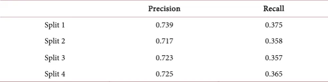
Table 7. Precision and recall values for the classification model on four random data splits.

Precision Recall

Split 1 0.739 0.375

Split 2 0.717 0.358

Split 3 0.723 0.357

Split 4 0.725 0.365

Table 8. Comparing observed and predicted component classes in a confusion matrix. Used to compute precision and recall values of classification model.

Predicted class

Observed class

Fault prone Non-fault prone Fault prone True negative (TN) False negative (FN) Non-fault prone False positive (FP) True positive (TP)

recall defined as 1) precision=TP÷

(

)

(

)

The intuition behind precision and recall is the following:

• _{Recall: how many fault-prone components our classifiers were able to}

identi-fy correctly as fault-prone.

• _{Precision: how many of the components classified by our classifiers as}

fault-prone are actually fault-prone.

DOI: 10.4236/jsea.2018.114010 163 Journal of Software Engineering and Applications the classification model is provided in Figure 2, which plots the Receiver Oper-ating Characteristic (ROC) metric. The area under the ROC curve (AUC) equals the probability that the classifiers predict a randomly chosen true positive higher than a randomly chosen false negative. The larger the AUC, the more accurate is the classification model. As shown in Figure 2, the accuracy of the classification model lies at 79% (AUC).

4.4. Study Validation

The validation of our study is based on the metrics validation methodology pro-posed by Schneidewind [22]. Following the Schneidewind’s validation scheme, the quality indicator is the pre-release fault density (F) and the metric suite (M) is the combination of the static analysis fault density together with the code com-plexity metrics. The six validation criteria are the following:

1) Association: “This criterion assesses whether there is a sufficient linear as-sociation between F and M to justify using M as an indirect measure of F” [22]. We identified a linear correlation between the pre-release fault density and the combination of the static analysis fault density with the code complexity metrics at a statistically significant level warranting the association between F and M.

2) Consistency: “This criterion assesses whether there is sufficient consisten-cy between the ranks of F and the ranks of M to warrant using M as an indirect measure of F” [22]. We demonstrated the consistency between the pre-release faults and the combination of static analysis fault density and code complexity metrics in Section 3 in Table 5.

3) Discriminative Power: “This criterion assesses whether M has sufficient discriminative power to warrant using it as an indirect measure of F” [22]. This is satisfied based on the results in Section 6, where we showed that discriminant analysis can classify effectively fault-prone from not fault-prone components.

DOI: 10.4236/jsea.2018.114010 164 Journal of Software Engineering and Applications 4) Tracking: “This criterion assesses whether M is capable of tracking changes in F (e.g., as a result of design changes) to a sufficient degree to warrant using M as an indirect measure of F” [22]. Table 6 justifies the ability of M to track F.

5) Predictability: “This criterion assesses whether M can predict F with re-quired accuracy” [22]. The correlation analysis results as well as the prediction analysis results in Section 3.

6) Repeatability: “This criterion assesses whether M can be validated on a sufficient percentage of trials to have confidence that it would be a dependable indicator of quality in the long run” [22]. We demonstrated the repeatability criterion by using random splitting techniques in Section 3. A limitation of our study with respect to repeatability is that all data used are from one software system.

5. Conclusions and Study Limitations

1) static analysis fault density combined with code complexity metrics can be used as an early indicator of pre-release fault density;

2) static analysis fault density combined with code complexity metrics can be used to predict pre-release fault density at statistically significant levels;

3) static analysis fault density combined with code complexity metrics can be used to discriminate between fault-prone and not fault-prone components.

This allows us to identify fault-prone components and focus most of the soft-ware quality assurance on such components. And this allows us to increase the effectiveness and efficiency of the expensive quality assurance tasks at Daimler.

The results reported in our study 1) are heavily dependent on the quality of the static analysis tools used at Daimler as well as the quality of the manual re-views executed to eliminate false positives, and 2) might not be repeatable with same degree of confidence with other tools. The defects detected by static analy-sis tools might be false positive. In our study, an internal review of the faults identified by static analysis tools has been executed, and only true positive faults have been used in this study. Moreover, it is possible that static analysis tools do not detect all faults during the development process. Such missed faults can be found by testing which would increase the pre-release fault density and conse-quently might perturbate the correlation. In order to mitigate possible skewness of the correlation, our hypothesis was that combining the static analysis fault density with code complexity metrics would account for faults not identified by static analysis tools. Although we could derive good predictors using this com-bination on the head unit control system at Daimler, this might not be genera-lizable to other software projects.

6. Future Work

al-DOI: 10.4236/jsea.2018.114010 165 Journal of Software Engineering and Applications so plan to extend the study by considering more data sources such as test cover-age metrics. We are also investigating criteria on assessing the similarities be-tween software projects, such as the polar chart proposed by Boehm et al.[23], where projects can be classified based on five dimensions (personnel, dynamism, culture, size, criticality). Such similarity criteria might allow us to increase the accuracy of the pre-release fault predictors across similar projects.

References

[1] Rana, R., Staron, M., Hansson, J. and Nilsson, M. (2014) Defect Prediction over Software Life Cycle in Automotive Domain State of the Art and Road Map for Fu-ture. 9th International Conference on Software Engineering and Applications, Vienna, 29-31 August 2014, 377-382.

[2] Haghighatkhah, A., Oivo, M., Banijamali, A. and Kuvaja, P. (2017) Improving the State of Automotive Software Engineering. IEEE Software, 34, 82-86.

https://doi.org/10.1109/MS.2017.3571571

[3] Singh, P., Pal, N.R., Verma, S. and Vyas, O.P. (2017) Fuzzy Rule-Based Approach for Software Fault Prediction. IEEE Transactions on Systems, Man, and Cybernet-ics: Systems, 47, 826-837.

[4] Nagappan, N., Ball, T. and Zeller, A. (2006) Mining Metrics to Predict Component Failures. Proceedings of the 28th International Conference on Software Engineer-ing, Shanghai, 20-28 May 2006, 452-461.

[5] Briand, L.C., Wüst, J., Ikonomovski, S.V. and Lounis, H. (1999) Investigating Qual-ity Factors in Object-Oriented Designs: An Industrial Case Study. Proceedings of the 21st International Conference on Software Engineeringin ICSE 99, Los Angeles, 22 May 1999, 345-354.

[6] Madureira, J.S., Barroso, A.S., do Nascimento, R.P.C. and Soares, M.S. (2017) An Experiment to Evaluate Software Development Teams by Using Object-Oriented Metrics. In: Gervasi, O., Murgante, B., Misra, S., Borruso, G., Torre, C.M., Rocha, A.M., Taniar, D., Apduhan, B.O., Stankova, E. and Cuzzocrea, A., Eds., Computa-tional Science and Its Applications, Springer International Publishing, Cham, 128-144.

[7] Subramanyam, R. and Krishnan, M.S. (2003) Empirical Analysis of CK Metrics for Object-Oriented Design Complexity: Implications for Software Defects. IEEE Transactions on Software Engineering, 29, 297-310.

[8] Tang, M.-H., Kao, M.-H. and Chen, M.-H. (1999) An Empirical Study on Ob-ject-Oriented Metrics. Proceedings of the 6th International Symposium on Software Metrics, Boca Raton, 4-6 November 1999, 242-249.

[9] Feist, J., Mounier, L., Bardin, S., David, R. and Potet, M.-L. (2016) Finding the Needle in the Heap: Combining Static Analysis and Dynamic Symbolic Execution to Trigger Use-after-Free. Proceedings of the 6th Workshop on Software Security,

Protection, and Reverse Engineering in SSPREW 16, Los Angeles, 5-6 December 2016, 1-12. https://doi.org/10.1145/3015135.3015137

[10] Avgerinos, T., Rebert, A. and Brumley, D. (2017) Methods and Systems for Auto-matically Testing Software. US Patent No. 9619375.

Relia-DOI: 10.4236/jsea.2018.114010 166 Journal of Software Engineering and Applications

bility Relevant Software Metrics. International Journal of System Assurance Engi-neering and Management, 8, 2097-2108.

[13] Denaro, G., Morasca, S. and Pezzè, M. (2002) Deriving Models of Software Fault-Proneness. Proceedings of the 14th International Conference on Software En-gineering and Knowledge EnEn-gineering in SEKE 02, Ischia, 15-19 July 2002, 361-368.

https://doi.org/10.1145/568760.568824

[14] Chidamber, S.R. and Kemerer, C.F. (1994) A Metrics Suite for Object Oriented De-sign. IEEE Transactions on Software Engineering, 20, 476-493.

https://doi.org/10.1109/32.295895

[15] Basili, V.R., Briand, L.C. and Melo, W.L. (1996) A Validation of Object-Oriented Design Metrics As Quality Indicators. IEEE Transactions on Software Engineering, 22, 751-761. https://doi.org/10.1109/32.544352

[16] Khoshgoftaar, T.M., Munson, J.C. and Lanning, D.L. (1993) A Comparative Study of Predictive Models for Program Changes during System Testing and Mainten-ance. In: Proceedings of the Conference on Software Maintenance, IEEE Computer Society, Washington DC, 72-79.

[17] Munson, J.C. and Khoshgoftaar, T.M. (1990) Regression Modelling of Software Quality: Empirical Investigation. Information and Software Technology, 32, 106-114.

[18] Jackson, J. and Edward. (2003) A User’s Guide to Principal Components of Wiley Series in Probability and Statistics. John Wiley & Sons, Hoboken.

[19] Jolliffe, I.T. and Cadima, J. (2016) Principal Component Analysis: A Review and Recent Developments. Philosophical Transactions. Series A, Mathematical, Physi-cal, and Engineering Sciences, 374, Article ID: 20150202.

https://doi.org/10.1098/rsta.2015.0202

[20] Nagappan, N., Williams, L., Hudepohl, J., Snipes, W. and Vouk, M. (2004) Prelimi-nary Results on Using Static Analysis Tools for Software Inspection. Proceedings of the 15th International Symposium on Software Reliability Engineering, Saint-Malo, 2-5 November 2004, 429-439.

[21] Nagappan, N. and Ball, T. (2005) Static Analysis Tools as Early Indicators of Pre-Release Defect Density. Proceedings of the 27th International Conference on Software Engineering, St. Louis, 15-21 May 2005, 580-586.

[22] Schneidewind, N.F. (1992) Methodology for Validating Software Metrics. IEEE Transactions on Software Engineering, 18, 410-422.