Quantifying and reducing Input modelling error in simulation

(1)

Quantifying and Reducing

Input Modelling Error in

Simulation

Lucy E. Morgan, B.Sc.(Hons.), M.Res

Submitted for the degree of Doctor of Philosophy at

Lancaster University.

(2)

This thesis presents new methodology in the field of quantifying and reducing input mod-elling error in computer simulation. Input modmod-elling error is the uncertainty in the output of a simulation that propagates from the errors in the input models used to drive it. When the input models are estimated from observations of the real-world system input modelling error will always arise as only a finite number of observations can ever be collected. Input modelling error can be broken down into two components: variance, known in the litera-ture as input uncertainty; and bias. In this thesis new methodology is contributed for the quantification of both of these sources of error.

To date research into input modelling error has been focused on quantifying the input uncertainty (IU) variance. In this thesis current IU quantification techniques for simula-tion models with time homogeneous inputs are extended to simulasimula-tion models with non-stationary input processes. Unlike the IU variance, the bias caused by input modelling has, until now, been virtually ignored. This thesis provides the first method for quantifying bias caused by input modelling. Also presented is a bias detection test for identifying, with controlled power, a bias due to input modelling of a size that would be concerning to a practitioner. The final contribution of this thesis is a spline-based arrival process model. By utilising a highly flexible spline representation, the error in the input model is reduced; it is believed that this will also reduce the input modelling error that passes to the simulation output. The methods described in this thesis are not available in the current literature and can be used in a wide range of simulation contexts for quantifying input modelling error and modelling input processes.

(3)

This thesis is dedicated to Jack.

“When life gives you lemons. Don’t make lemonade. Make life take the lemons back!”

(4)

I would firstly like to thank STOR-i CDT for the numerous opportunities they have given to me throughout my MRes and PhD, I also gratefully acknowledge the financial support of the EPSRC. Being part of STOR-i has been an absolute pleasure. The support of the staff and students has helped me both academically and personally in many ways over the last four years. I’m grateful to all the people I’ve been lucky enough to share this process with. Doing a PhD is no easy task and I’ve loved being able to smile, laugh and, at times, cry with my STOR-i family. I’d like to add a special thanks to a few people in STOR-i who have made my time here brighter. To Kathryn for all the laughter, you’ve been a true friend. To Luke, my “academic brother”, I wish you all the success in the years ahead. To Emma and Emily thank you for introducing me to the country music that helped me dance my way through the last few months. To Jake thank you for all the silliness, I know you’re going on to great things. And finally to Helen and Katie, I can’t be thankful enough I had two such great friends to pick me up when times were hard and to celebrate the best times.

Of course I wouldn’t have left square one without the support of my three amazing su-pervisors. I’ve been so very lucky to work with you all. I’d firstly like to thank Dr Andrew Titman for all his help, patience and his deep understanding of statistics, I can’t promise I won’t be knocking on your door in future. Secondly I’d like to thank Dr David Worthington for his continuing support. I chose my PhD project because I felt we’d work well together, I wasn’t wrong, and I hope there are opportunities to continue to work together in future. Lastly I’d like to thank Professor Barry Nelson for stretching my research ability and help-ing me to achieve higher than I ever thought possible. Takhelp-ing on a student from a different

(5)

IV

continent was a large commitment, I hope you’ve enjoyed the process as much as I have! Special thanks also go to Jeanne Nelson for giving me such a warm welcome on my visits to Chicago.

The PhD process has seen me go through some of my biggest ups and downs and so a massive thank you has to go to my partner in crime Alec for making me smile daily. I wouldn’t be at the finish line without your support. Seeing you finish your PhD I knew this process would be hard and I’m so glad I had you by my side through it all. I’m excited to see what our future holds.

(6)

I declare that the work in this thesis has been done by myself and has not been submitted elsewhere for the award of any other degree.

This thesis is constructed as a series of papers. Chapters 3, 4 and 5 should therefore be read as separate entities.

Chapter 3 has been published as Morgan, L. E., Nelson B. L., Titman A. C. and Worthing-ton D. J. (2016). Input Uncertainty Quantification for Simulation Models with Piecewise-constant Non-stationary Poisson Arrival Processes. InProceedings of the 2016 Winter Sim-ulation Conference, pages 370-381. IEEE Press.

An early version of Chapter 4 was published as Morgan, L. E., Nelson B. L., Titman A. C. and Worthington D. J. (2017). Detecting Bias due to Input Modelling in Computer Simu-lation. InProceedings of the 2017 Winter Simulation Conference, pages 1974-1985. IEEE Press. An extended version of this paper was then submitted for publication as Morgan, L. E., Nelson B. L., Titman A. C. and Worthington D. J. (2018). Detecting Bias due to Input Modelling in Computer Simulation.European Journal of Operational Research. This sub-mission is currently under revision.

The word count for this thesis is 42,131 words.

Lucy E. Morgan

(7)

List of Figures

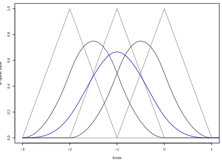
2.4.1 A single cubic B-spline (blue) and the lower degree, quadratic (dark grey)

and linear (light grey), B-splines from which it is composed. . . 28

2.4.2 The support of n=7 B-splines over the interval [0,3) given uniform knot vectorsss={−3,−2,−1,0,1,2,3,4,5,6,7} . . . 29

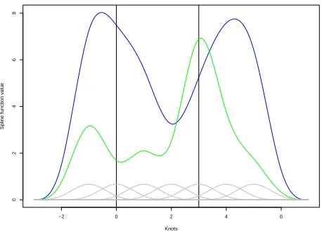
2.4.3 Two cubic spline functions (green and blue) on knot vectorsss={−3,−2,−1,0,1, 2,3,4,5,6,7}with spline coefficientsccc₁={9.02,7.46,6.04,2.04,5.34,8.13,7.61} (blue) andccc2={4.57,0.69,2.80,0.70,9.45,2.80,1.94}(green) along with the B-spline basis functions from which they were composed (grey). . . 30

2.4.4 Two spline functions (green and blue) on knot vector sss={−2.0, −1.5, −1.0, −0.5,0.0,0.5,1.0,1.5,2.0,2.5,3.0,3.5,4.0,4.5,5.0,5.5,6.0,6.5,7.0,7.5,8.0} along with the B-spline basis functions from which they were composed (grey). . . 30

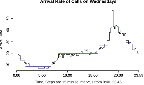
3.4.1 Change point analysis on the arrival rate of calls on Wednesdays. . . 47

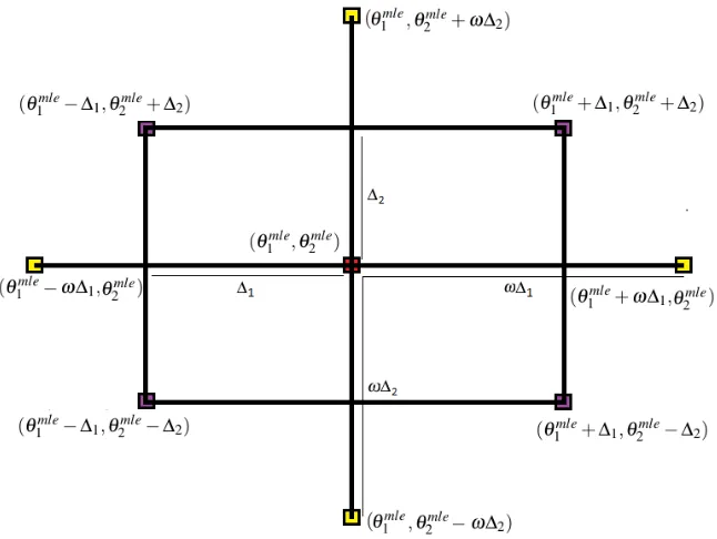
4.3.1 A CCD design with dimensionk=2. . . 59

4.4.1 M/M/1/10 . . . 72

4.4.2 M/M/1/100 . . . 72

4.4.3 The true response surfaces plotted over the CCD design space. Top left: linear, Equation (4.4.3); top right: quadratic, Equation (4.4.4); bottom left: cubic, Equation (4.4.5); and bottom right: cubic, Equation (4.4.6). The point(θ₁c,θ₂c)is marked in blue. . . 74

(12)

4.4.4 The average arrival counts over 96, 15 minute, intervals given m_d days of arrival data. Intervals post pre-processing of the data using change-point analysis are shown in blue. . . 80

5.4.1 The kth spine function component plus, a piecewise-constant majorising function (red) and an example of a piecewise-linear majorising function (blue) that could be used to generate arrivals via inversion using the method of Klein and Roberts (1984). . . 98 5.5.1 m_d=15,κ=5,ξ =1 - SPL (blue), PQ (green) and PL (red) . . . 104

5.5.2 m_d=100,κ=1,ξ =10 - SPL (blue), PQ (green) and PL (red) . . . 105

5.5.3 Pairwise comparison of the three methods using scatter plots of the integrated ab-solute difference, δ, over G=500 replications of the NHPP fit. Heremd =15,

κ=5 andξ =1. . . 106

5.5.4 Pairwise comparison of the three methods using scatter plots of the maximum absolute difference,ζ, overG=500 replications of the NHPP fit. Heremd =15,

κ=5 andξ =1. . . 106

5.5.5 Pairwise comparison of the three methods using scatter plots of the integrated ab-solute difference,δ, overG=500 replications of the NHPP fit. Heremd=100,

κ=1 andξ =10. . . 107

5.5.6 Pairwise comparison of the three methods using scatter plots of the maximum absolute difference,ζ, overG=500 replications of the NHPP fit. Heremd=100,

κ=1 andξ =10. . . 107

(13)

List of Tables

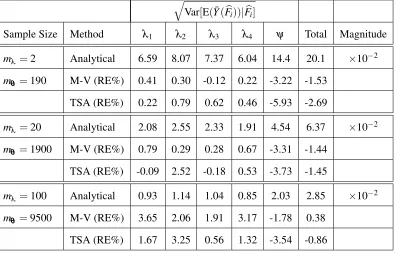
3.4.1 Experiment 1(i): The analytical contribution of theithinput distribution and the percentage relative errors of the M-V and TSA methods when the arrival process isλ(t) = 1₃,1₂,₁₂5,₃1and service rateψ =0.2. Here E(N) =¯ 1.94. 45

3.4.2 Experiment 1(ii): The analytical contribution of the ith input distribution and the percentage relative errors of the M-V and TSA methods when the arrival process isλ(t) = ₁₂1,1₈,₄₈5,₁₂1and service rate isψ =0.05. Here

E(N) =¯ 1.84. . . 46 3.4.3 The effect of different staffing schemes on the parameter contribution for

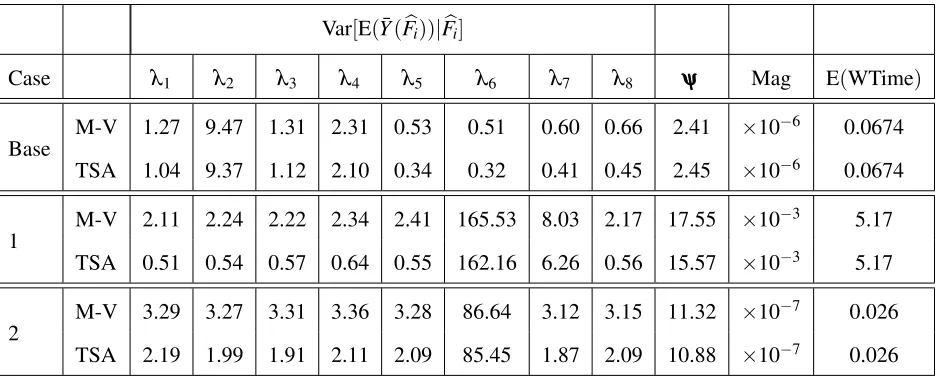
input distributions, Var[E(Y¯(Fbi))|Fbi],i=1,2, . . . ,p. . . 49 4.4.1 How power holds whenγ =bapproxgiven a truly quadratic response function. 69

4.4.2 How power holds whenγ =bapproxgiven anM/M/1/Cqueueing model. . 71

4.4.3 Bias test results varying the form ofη(·), the amount of input data,m, and number of replications,r. Herepband LOF are the fraction out ofG=1000

macroreplica-tions that the bias test and lack-of-fit test, respectively, rejected their null hypothe-sis, andbb¯ is the average bias estimate. . . 76

4.4.4 The bias detection test in a NHS 111 healthcare call centre scenario consid-ering the expected waiting time of callers, E(WTime), with m_d =10 and

m_d=26 days of arrival data. Results for both the bias and the lack-of-fit tests are presented. . . 81

(14)

5.5.1 The average maximum absolute difference, ¯ζ, the average integrated

abso-lute difference, ¯δ, and the coefficient of variation of the integrated absolute

difference,ι, for the fit of two arrival rate functions givenmd,κ andξ. . . 101 5.5.2 The average maximum absolute difference, ¯ζ, the average integrated

difference,ι, for the fit of two arrival rate functions given different settings

ofm_d,κ andξ for underdispersed data. . . 111

5.5.3 The average maximum absolute difference, ¯ζ, the average integrated

difference,ι, for the fit of two arrival rate functions given different settings

ofm_d,κ andξ for overdispersed data. . . 112

B.1 In G=500 fits of the arrival rate function, the proportion of times the spline-based input model, “SPL”, achieved the smallest maximum gap,ζ, or integrated

absolute gap,δ, compared to the piecewise-linear, “PL”, and piecewise-quadratic,

“PQ”, input models.. . . 134 B.2 Given underdispersed observations with targetcv=0.52. InG=500 fits of the

arrival rate function, the proportion of times the spline-based input model, “SPL”, achieved the smallest maximum gap,ζ, or integrated absolute gap,δ, compared to

the piecewise-linear, “PL”, and piecewise-quadratic, “PQ”, input models. . . 135 B.3 Given overdispersed observations with target cv=1.52. In G=500 fits of the

arrival rate function, the proportion of times the spline-based input model, “SPL”, achieved the smallest maximum gap,ζ, or integrated absolute gap,δ, compared to

(15)

Introduction

1.1 Motivation

Stochastic simulation is a tool used to aid decision making. It allows practitioners to analyse and experiment with systems that are driven by random processes. For systems where the performance measures of interest are mathematically intractable, stochastic simulation is a natural choice. In practice simulation is used in many industries to study complex systems, examples include: healthcare (Brailsford, 2007), aviation modelling and analysis (Rhodes-Leader et al., 2018) and manufacturing (Law, 1988).

The conclusions drawn from simulation experiments are conditional on the input mod-els that drive them. Typically these input modmod-els, represented by probability distributions or processes, are estimated using observations collected from the real-world system using sta-tistical methods such as maximum likelihood estimation. When this is the case uncertainty arises in the estimated input models due to the fact that only a finite number of observations can be collected from the system of interest. As the amount of input data increases the error in the input models decreases, but they are never perfectly correct. In experiments where constraints on time and money have limited the number of observations collected from a system, the error in the input models can be substantial. For example, in a manufacturing

(16)

context the pressure to make a timely decision about whether to switch to a new method of production may limit the time available to observe and model the various manufacturing processes.

In this thesis the error that propagates through a simulation model, from the estimated input models to the performance measures under study, is referred to as the error caused by input modelling. In practice ignoring error caused by input modelling can lead to over-confidence in the decisions supported by the simulation. The problem of quantifying and reducing the error in the output of a simulation caused by error in the input models therefore motivates this thesis.

In recent years there has been substantial interest in quantifying the variance caused by input modelling in a simulation response. In the simulation community this variance is known as input uncertainty. Unlike stochastic uncertainty, which can be reduced by per-forming additional replications of the simulation, input uncertainty can only be reduced by collecting further observations of the system to gain better estimates of the input mod-els. Methods for input uncertainty quantification for simulation models with homogeneous inputs exist, and one such method, proposed by Song and Nelson (2015), has been imple-mented in the commercial software Simio (2015). Despite nonhomogeneous input models commonly being used in simulation experiments, input uncertainty quantification for non-homogeneous input models is yet to be addressed. One focus of this thesis is therefore the quantification of input uncertainty for simulation models with non-homogeneous Poisson processes.

(17)

CHAPTER 1. INTRODUCTION 3

caused by input modelling, but when the number of observations is finite nothing can be said about the relative size of bias and input uncertainty and it therefore should not be ignored.

In simulation in practice a common way of representing a nonhomogeneous arrival process is to use a nonhomogeneous Poisson process (NHPP). Substantial research has been carried out into fitting the arrival rate function, λ(t), and integrated rate function,

Λ(t), of a NHPP to observed data, and for simulating arrivals from these representations

using techniques such as thinning and inversion. The common use of NHPPs in practice has also led to their availability in commercial simulation software. Given the value of NHPPs as input models to simulation there is a motivation to create an input modelling method that recovers the true arrival rate function of a NHPP “better” than existing methods. By reducing the error between the true input model and the fitted model a reduction in the error caused by input modelling should be seen in the simulation output. Providing practitioners with the tools to quantify and reduce the error in the simulation output caused by input modelling would improve their ability to make decisions with the support of simulation.

The outputs of this thesis are threefold. First, new methodology for the quantification of input uncertainty in simulation models with non-stationary input processes is presented. Second, new methodology for detecting the bias caused by input modelling on the output of simulation is presented. Finally, a new spline-based input modelling method for the arrival rate of a NHPP is developed.

1.2 Contributions

We now outline for the reader the main contributions of this thesis.

(18)

non-stationary Poisson arrival processes. In practice arrival processes to simulation models are often nonhomogeneous with respect to time. Numerical evaluation and illustrations of the methods are provided and indicate that the methods perform well.

Our second contribution is to provide the first method for quantifying bias caused by input modelling. This also provides the first way to summarise the mean squared error caused by input modelling for a simulation performance measure by bringing together the input uncertainty variance and the squared bias. As the key to this contribution a bias detection test is also presented with controlled power for detecting bias of a size that exceeds a threshold deemed to be concerning by a practitioner. We numerically evaluate the bias detection test and demonstrate its use in a realistic case study concerning a healthcare call centre.

The final contribution of this thesis is a spline-based arrival process modelling method. Specifically we develop a new method for representing the arrival rate function of a NHPP and a simple method for simulating arrivals from it. By using a spline function represen-tation with a large number of knots we reduce the bias, with respect to the true arrival rate, in the model. The more knots used to build the spline function the more flexible it can become, we therefore control over fitting, and thus variability, by penalising the NHPP log-likelihood when fitting the spline function. By aiming to reduce the error in the arrival process model, we also reduce the input modelling error passed to the simulation output. To evaluate this model we compare it to the methods of Zheng and Glynn (2017) and Chen and Schmeiser (2017), from the arrival process modelling literature, and demonstrate the use of the spline-based input model using observations from a real-world A&E department with a cyclic arrival rate function.

1.3 Outline of Thesis

(19)

CHAPTER 1. INTRODUCTION 5

(20)

In this chapter the reader is provided with the necessary background material, including references to useful sources, to aid the understanding of this thesis. Firstly the concept of nonhomogeneous Poisson processes (NHPPs), how to check real-world data follows a NHPP and techniques for simulating data from a NHPP are introduced. Secondly, input modelling is discussed with specific detail on modelling the arrival rate and integrated rate functions of a NHPP. The idea of error caused by input modelling is then introduced along-side definitions of input uncertainty and bias caused by input modelling. Finally spline functions and B-spline basis functions are introduced.

2.1 Nonhomogeneous Poisson processes

The focus of this thesis is on the simulation of systems with input processes that can be appropriately described by non-homogeneous Poisson processes (NHPPs). In reality, ar-rivals to a system are often known to be non-stationary; NHPPs are a common model used to describe the arrival process when this is the case. For example, Pritsker et al. (1996) used NHPPs for fitting donor and patient arrivals within a large scale simulation model de-veloped for the United Network of Organ Sharing (UNOS). NHPPs can be used to model many types of non-stationary arrival process and are therefore appropriate for use in many

(21)

CHAPTER 2. BACKGROUND MATERIAL 7

application areas including: manufacturing (Viswanadham and Narahari, 1992), healthcare (Green, 2006), and call centres (Kim and Whitt, 2014).

A NHPP is a generalisation of a homogeneous Poisson process. For a homogeneous Poisson process events are said to occur at a constant rateλ per unit time. In a NHPP this

rate, or intensity, λ(t), is allowed to change through time and is assumed non-negative, λ(t)≥0, for allt (Kingman, 1992). Given two points a andb, where a≤b, let N be a

NHPP andN(a,b)denote the number of events on interval(a,b]. By definition of a NHPP, the number of observations in interval(a,b],N(a,b), follows a Poisson distribution

N(a,b)∼Pois(Λ(a,b))

where the probability ofsevents occurring on interval(a,b]is

P(N(a,b) =s) = exp{−Λ(a,b)}Λ(a,b) s

s! . (2.1.1)

HereΛ(a,b)is known as the integrated rate, or cumulative intensity function and is defined

by

Λ(a,b) =

Z b

a

λ(t)dt.

Within interval(a,b], Λ(a,b) can be interpreted as the expected number of observations Λ(a,b) =E[N(a,b)]. When considering the expected number of observations up to timet, Λ(0,t) =R₀tλ(s)dslet the integrated rate function be denoted byΛ(t).

Another property of a NHPP is that the sum ofqindependent NHPPs is also a NHPP,

N=N1+N2+· · ·+Nq,

where N_i for i =1,2, . . . ,q are NHPPs, see Blumenfeld (2009). When this is the case the rate, or intensity, function ofN can also be decomposed into the sum of the intensity functions of itsqcomponents

λc(t) =λ₁c(t) +λ₂c(t) +· · ·+λ_qc(t),

(22)

In simulation it is important to model an input process as nonhomogeneous if it is so. Arrivals to systems in the real-world are often seen to vary through time. Estimating the distribution of these arrivals using a homogeneous distribution would remove any fluctu-ations in the arrival process; this may have a large impact on the output measures of the simulation. For example, in a call centre there are usually times of the day where the arrival rate of calls peaks and troughs. A constant arrival rate would therefore not represent the true arrival rate to this system well; and would lead to over or under staffing, see Whitt (2007). In Chapter 3 the arrival rate to a healthcare call centre is used to guide the number of staff to have on duty. This can be seen to have a large effect on the expected waiting time of callers when comparing the use of homogeneous and nonhomogeneous arrival processes as inputs to the simulation.

2.1.1 Real-world observations

For a NHPP, denotedN, the number of arrivals during interval(a,b], denotedN(a,b), fol-lows a Poisson distribution. Therefore the dispersion, or variance-to-mean ratio, of the number of arrivals during an interval,ω=E[N(a,b)]/Var[N(a,b)], should equal 1. This is

not guaranteed given real-world data, even when the underlying process is a NHPP. Arrival processes in practice can be both under (ω<1) or over (ω>1) dispersed in comparison to

a NHPP. It is therefore sensible to perform checks on the real-world observations to confirm the appropriateness of modelling an input as an NHPP.

One way to check whether the observed data within an interval,(a,b], follow a NHPP is to record the arrival counts to the interval multiple times and use a chi-square goodness-of-fit test to check whether this data comes from a Poisson distribution. The chi-square test for supposedly Poisson data compares the observed counts over an interval,O_i, to the expected count,Ei, assuming the data came from a Poisson distribution. For example, given observations of arrivals to an A&E department on Mondays over w weeks the following hypothesis

(23)

would be tested against

H1: The total number of arrivals on Monday is not Poisson.

with test statistic,T,

T = w

∑

i=1

(Oi−Ei)2 E_i .

Note that the expected number of arrivals on a Monday can be estimated by the mean of the observed countsE_i=O¯= _w1∑w_i₌₁Oi. In comparing the test statistic,T, to the critical value

ψ, of the chi-squared distribution with w−1 degrees of freedom at the α% significance

level, ifT <ψthere is not significant evidence to reject the null hypothesis that the observed

counts are from a Poisson distribution. Of course the chi-square goodness-of-fit test is not a guarantee that the observed data is Poisson but, when the null hypothesis is rejected, this indicates that the data is not Poisson; the test is therefore a good warning tool. Another consideration in using the Chi-squared test is that the number and location of the intervals may not be known. In practice they may have to be chosen by the practitioner which introduces subjectivity into the approach.

2.1.2 Generating arrivals

Simulating a homogeneous Poisson process is relatively simple. The inter-arrival time be-tween consecutive customers is known to be an exponential random variable with cumu-lative density function (cdf)F(t) =1−exp{−λt}, t≥0. Simulation of theith customers

arrival time is therefore simply

yi=yi−1+F−1(s) =yi−1−

ln(1−u_i)

λ

(24)

Inversion

Inversion is so called due to its dependence on the the inverse of the integrated rate function,

Λ−1(t). Cinlar (2013) proves that random variablesTi, i=1,2, . . . are arrival times from a NHPPN with integrated rate functionΛ(t)if and only ifΛ(T1),Λ(T2), . . . are event times

from a stationary Poisson process with rate one. This holds for all t ≥0 when Λ(t) is

a positive-valued, continuous, non-decreasing function. Inversion therefore requires the integrated rate functionΛ(t)to be invertible. When it is possible to calculate this inverse,

the method proceeds as follows:

1. Generate random variableu_i∼Uniform(0,1).

2. Generate Poisson arrival times with rateλ =1 usingy0=0,yi=yi−1−ln(1−ui). 3. Calculate theitharrival time from the NHPP,ti, byti=Λ−1(yi).

One problem with inversion is that the integrated rate function,Λ(t), will not always have

a tractable inverse. Although there may be no tractable functional form for Λ−1(t), the

integrated rate function will always be numerically invertible. Numerical inversion in this case is equivalent to a one-dimensional search. To account for possible flat regions of the integrated rate function a generalised definition of the inverse integrated rate function is used,

Λ−1(t) =inf{x∈_R:Λ(x)≥t}.

For generating a single arrival the numerical search for the inverse should be reasonably quick but, within a simulation model, it is quite possible that thousands of arrivals will be required in which case completing a search for each arrival will add up. A common approach to improve efficiency in this case is to numerically evaluateΛ−1(t)over a grid of

points and linearly interpolate between these.

WhenΛ(t)is easily invertible, inversion is a simple efficient way of generating arrivals

(25)

is piecewise-quadratic within each interval and thus a tractable inverse function exists from which to generate arrivals from the underlying NHPP.

Thinning

Thinning is an arrival generation method for NHPPs that works directly with the rate func-tion, λ(t). The key idea is to generate arrivals from an alternative function that is both

simpler to generate arrivals from and that majorises the original function of interestλ(t).

The arrivals generated from the alternative function are then ‘thinned’, some are thrown out, according to the probability that they came from the NHPP with arrival rateλ(t).

Like inversion, thinning traditionally begins with the generation of arrivals from a sta-tionary Poisson process but in this case the stasta-tionary arrival process has arrival rate equal to the maximum rate, maxtλ(t) =λ?. Arrivals are discarded according to the probability

of them having come from the NHPP. Specifically an arrival at timet is rejected according to a Bernoulli trial with success probabilityλ(t)/λ?. The probability that a potential arrival

is thinned is thus 1−λ(t)/λ?. The discrepancy betweenλ?and the arrival rate function of

interestλ(t)has a large effect on how many arrivals are rejected and thus the efficiency of

the method. For an algorithm of how to implement thinning see Nelson (2013). A proof that the thinning method samples from a NHPP with rateλ(t)is omitted here but a sketch proof

can be found in Kuhl and Wilson (2009). One advantage of this approach is that thinning can be used to generate arrivals from any bounded arrival rate functionλ(t); complexity

is not an issue. Although, it may be said that thinning is a wasteful method. For example, if the rate function of interest has a high peak with short duration and the rest of the pro-cess is a much lower rate then thinning usingλ?=maxtλ(t) could be highly inefficient, discarding a high proportion of simulated points.

(26)

majorising function can be thinned in the same way as the arrivals from a constant majoris-ing function. Let ˜λ(t)denote the piecewise-linear majorising function, then the probability

of thinning a potential arrival is 1−λ(t)/λ˜(t). As before, thinning arrivals generated from

˜

λ(t)gives arrivals from the arrival process with arrival rateλ(t).

The methods of thinning and inversion both lead to an arrival process with the specified arrival rateλ(t), but this does not mean that the arrivals generated using the methods will be

the same. This is due to the stochastic variability in how the arrivals are generated between the two methods. Methods for modelling the rate,λ(t), or integrated rate,Λ(t), function of

a NHPP will now be discussed.

2.2 Input Modelling

In this thesis “input modelling” refers to the method of forming a representation of an input to a simulation model from which event times can be generated. The focus of this thesis is on the estimation of input models using data. Sometimes data are unavailable and subjective decisions have to be made about certain inputs; from here on in inputs created in this way are not considered and focus lies on input models that have been estimated using observations from the system of interest.

This section reviews relevant methods within the input modelling literature with spe-cific focus on methods for modelling and generation of NHPPs, as introduced in §2.1. For a more general discussion of input modelling techniques for use in discrete event simula-tion see Leemis (2001) and Cheng (2017), see also Cheng (1994) for a discussion of how to select appropriate input distributions. When arrival observations are over or under dis-persed compared to a Poisson process, Gerhardt and Nelson (2009) present methodology for modelling non-stationary non-Poisson arrival processes and Nelson and Gerhardt (2011) consider the modelling and simulation of non-stationary, non-renewal processes. For a dis-cussion of input modelling for complex problems see Nelson and Yamnitsky (1998).

(27)

rate function, λ(t), or integrated rate function, Λ(t) (Kuhl and Wilson, 2009), any input

modelling approach for a NHPP aims to estimate one of these functions. The existing input modelling literature will now be summarised.

2.2.1 Estimating the rate function,

λ

(

t

)

A common, early, approach to estimating the intensity function, λ(t), of a NHPP was to

use an exponential form. Exponentiating the rate function ensures it is always non-negative,

λ(t)≥0. This idea was first considered by Cox and A. W. Lewis (1966) who stated that a

continuous rate function for a NHPP can be estimated arbitrarily closely with an exponential polynomial function. This idea was built upon by Lewis (1971), Lewis and Shedler (1976), Lee et al. (1991) and Kuhl et al. (1997). The key idea is to model the intensity function by fitting an exponential function with some additional components to reflect knowledge about the underlying process. For example, Kuhl et al. (1997) present the exponential-polynomial-trigonometric rate function with multiple periodicities (EPTMP)

λ(t) =exp

l

∑

j=0

αjtj+ p

∑

k=1

γksin(ωkt+φk) !

, (2.2.1)

which can handle NHPPs where the arrival rate exhibits trends and multiple-periodicities. All exponential forms of the rate function are parametric and require the estimation of parameters when being fit to data. For example, for the EPTMP rate function (2.2.1), esti-mation of the parameters{α0,α1, . . . ,αl,γ1,γ2, . . . ,γp,ω1,ω2, . . . ,ωp,φ1,φ2, . . . ,φp}would be required to fit the rate function. Numerically optimising these parameters is computa-tionally expensive and often requires a good starting point.

Another common approach to modelling both the rate function,λ(t), and the integrated

rate function,Λ(t), is to assume they take a piecewise form. Henderson (2003) considered

(28)

(2005) and Avramidis et al. (2004) who both use a piecewise-constant arrival rate in a call centre setting.

Massey et al. (1996) present a piecewise-linear representation of the arrival rate function given arrival count data. They fit the rate function using ordinary least squares (OLS), iterative weighted least squares (IWLS) and maximum likelihood (ML) where all methods are constrained to yield a non-negative rate function. More recently, Nicol and Leemis (2014) used count observations to provide a piecewise-linear estimator of the rate function,

λ(t). This method was formulated as a constrained quadratic programming problem with

constraints on the continuity of the estimator, the estimator’s mean value within an interval and optional constraints on the interval end points for cyclic contexts.

Chen and Schmeiser (2013) present an iterative algorithm for smoothing a piecewise-constant representation of the intensity function. Within each iteration they run their algo-rithm, Smoothing via Mean-constrained Optimized-Objective Time Halving (SMOOTH), which takes a piecewise constant arrival rate function and yields a ‘smoother’ represen-tation with double the number of intervals, each with half the length. Here smoothness is measured in terms of the integrated squared second derivatives. The resulting repre-sentation is non-negative and maintains the integral of the original function and thus the expected number of arrivals in each interval. Iteration of the SMOOTH algorithm gives the proposed, I-SMOOTH method which returns a sequence of sequentially smoother arrival rate functions. The method is aimed to be automatic, but the user is required to set how many iterations to let I-SMOOTH carry out.

(29)

inter-CHAPTER 2. BACKGROUND MATERIAL 15

valsι given a total ofaarrival times is

bι≡argminι=1,2,...ι(2a− ι

∑

j=1

(C_j(ι)2))

whereC_j(ι) is the number of arrivals in the jth interval when there are ι intervals. This

method could act as a pre-processing step for input modelling modelling methods, like I-SMOOTH, that assume the underlying NHPP has a piecewise form and that the number of intervals and interval locations are known.

As for higher order polynomial representations. Kao and Chang (1988) present a piece-wise polynomial representation by ‘grafting’ polynomials of different degrees together whilst constraining the continuity of the resulting representation. The method is subjec-tive in the choice of polynomial degree in each interval, and the break points at which the function changes.

In Chapter 5 a spline-based method for modelling and generating NHPPs is developed and compared to two recent methods in the literature: a piecewise-linear representation by Zheng and Glynn (2017) and a piecewise-quadratic representation by Chen and Schmeiser (2017). Both competing methods allow estimation of a NHPP intensity function from ar-rival time observations and both can be used alongside the pre-processing method of Chen and Schmeiser (2018).

Zheng and Glynn (2017) assume the underlying rate function of the NHPP is piecewise-linear and that the placement and number of intervals is known. They provide two methods for fitting the intensity function, one using maximum likelihood estimation, and one using ordinary least squares (OLS) methods. Given the assumed piecewise-linear form of the rate function they reduce the problem of estimatingλ(t)to estimating the arrival rate at the

(30)

maximum likelihood optimisation problem is given by

max

y0,y1,...,yp

L_m(y₀,y₁, . . . ,y_p)

s.t. y₀=y_p

y_i≥0, 0≤i≤ p

wherey0,y1, . . . ,ypare the arrival rates at the interval boundaries andLm(·)is the likelihood givenmobservations of the NHPP. The structure of this problem means that even for large mand moderate pthe problem is computationally tractable.

Chen and Schmeiser (2017) present the Max Nonnegativity Ordering Piecewise-Quadratic Rate Smoothing (MNO-PQRS) algorithm, for general input processes, which takes a piecewise-constant representation of the rate function and returns a smoother, piecewise-quadratic function. The algorithm is not specific to NHPPs and requires no user specified parame-ters. It smooths the arrival rate function whilst maintaining the expected number of arrivals in each interval. MNO-PQRS has two components: first, the Piecewise-Quadratic Rate Smoothing (PQRS) algorithm smooths the initial piecewise-constant representation return-ing a continuous, differentiable rate function. Then, if PQRS returns any negative sections of the rate function, the Max Nonnegativity Algorithm (MNO) returns the maximum of zero and the PQRS representation. Like the I-SMOOTH method by Chen and Schmeiser (2013) the method requires an initial piecewise-constant representation to be known; this could be provided by the pre-processing method of Chen and Schmeiser (2018).

Another approach for fitting a NHPP rate function was presented by Kuhl and Bhair-gond (2000) who construct a highly flexible NHPP rate function representation using wavelets. Their method has the advantage of requiring no prior knowledge or assumptions to be made about the behaviour of the process.

(31)

fitting their spline function they use a recurrence relation to reduce their problem to a linear system of equations which they solve by Gaussian elimination.

2.2.2 Estimating the integrated rate function,

Λ

(

t

)

An alternative to estimating the rate function,λ(t), of a NHPP is estimation of the

cumu-lative rate function,Λ(t). For the cumulative rate function there is a natural estimator,

cal-culated from the observed data, known as the empirical cumulative rate function (ECRF). There is no counterpart of the ECRF for the rate function. The ECRF is a step function with each step corresponding to either an arrival to the system or a count of arrivals in an interval given observations of the input process. This method of modelling the cumulative rate function may be thought of as crude, but as the number of observations increases the bias reduces. The ECRF also has no dependency on the input process following Poisson assumptions.

When the input process is a NHPP, Leemis (1991) presents a non-parametric piecewise-linear estimator of the cumulative intensity function,Λ(t). The method essentially linearly

interpolates the ECRF function between ordered event times. Generation of event times from the NHPP given the piecewise-linear representation using inversion is also discussed. Arkin and Leemis (2000) extend this method to include overlapping realisations, the key to their method being to partition the observation interval into the smallest number of regions so that, within each region, there are a constant number of realisations observed.

Given observations of event counts Leemis (2004) presents a maximum likelihood esti-mator of the cumulative intensity function,

b

Λ(t) =

i−1

∑

j=1

n_j k

!

+ ni(t−ai) k(ai−ai−1)

fora_i₋₁<t≤a_i.

(32)

to large variability in the estimator. If the subinterval lengths are too large, interesting features, for example trends and cycles, in the data may be missed.

Kuhl and Wilson (2000) investigate least squares methods for fitting the integrate rate function,Λ(t), with rate function of the EPTMP form, as in Equation (2.2.1).

The idea of quantifying the error caused by input modelling that propagates through a simulation model to the simulation output performance measures is now introduced.

2.3 Error Caused by Input Modelling

The “stochastic” in stochastic simulation is a reflection of the input models that are used to drive a simulation through time. Input modelling, as discussed in Chapter 2.2, allows us to form representations of the inputs to a simulation model; this may, for example, be in the form of a statistical distribution, empirical distribution or statistical process. These representations are formed using observations of the system of interest and thus, since only a finite number of observations can ever be collected, contain error. In this thesis the error that propagates to the simulation output due to there being error in the input distributions that drive the simulation is referred to as the error caused by input modelling.

(33)

increased; error caused by input modelling does not.

In practice, quantification of the error in simulation responses has mainly been restricted to quantifying the SEE. Barton (2012) warns of the danger of not considering error caused by input modelling and Lin et al. (2015) show that error caused by input modelling can be many orders of magnitude larger than SEE. Ignoring error caused by input modelling can lead to over-confidence in the output of the simulation especially when there is little data from which to estimate the input distributions and a large amount of simulation effort has been spent on reducing the SEE.

The mean squared error (MSE) error caused by input modelling can be broken down into variance, known in the literature as input uncertainty (IU), and the squared bias caused by input modelling

MSE=Input Uncertainty+Bias2.

The methodology behind input uncertainty quantification and bias caused by input mod-elling shall now be considered.

2.3.1 Input Uncertainty

First let us formally introduce and define input uncertainty. For simplicity, consider a simulation model with a single input, with true distribution Fc, from which i.i.d data X₁,X₂, . . . ,X_m has been sampled. The true distribution,Fc, from which these values were sampled is unknown, it is therefore estimated by fitting distribution F, a function of theb observed data. In practiceFbis used to drive the simulation model; let the observed output of the simulation in replication jbe denoted

Y_j(F) =b η(Fb) +ε_j(Fb)

whereη(Fb)is the expected simulation response dependent on the estimated distributionFb andε1(F)b ,ε2(Fb), . . . ,εn(F)b are i.i.d random variables representing the noise from replica-tion to replicareplica-tion of the simulareplica-tion with mean 0 and varianceσ2. In practice this noise is

(34)

simulation to, for example, generate event times. In running the simulation, our interest is in estimating the expected simulation response,η(Fb), which may be estimated by taking the average of the simulation output overnreplications

¯ Y(Fb) =

1 n

n

∑

j=1

Y_j= 1 n

n

∑

j=1

η(F) +b ε_j(F)b

=η(Fb) + 1 n

n

∑

j=1

εj(Fb).

As the number of replications,n, gets large the noise in the simulation is driven down to 0. The variability in ¯Y(F)b can be broken down, using the total law of variance, into input uncertainty and stochastic estimation error as follows

Var(Y¯(F)) =b Var[E(Y¯(Fb)|F)] +b E[Var(Y¯(F)b |Fb)]. (2.3.1) Input uncertainty, the first term in Equation (2.3.1), is the variability in ¯Y(F)b that comes from having estimated the input distributions. Since the fitted distribution,F, is based onb real-world data it is independent of the noise in the simulation and thus IU reduces to

IU=Var[η(F)]b . (2.3.2)

The second term in Equation (2.3.1) represents the SEE that arises in the simulation model, it can be estimated using the sample variance of the simulation response,S2/n.

(35)

to use bootstrapping, see Efron and Tibshirani (1986), which is the basis for their second approach. Bootstrapping mimics the effect of having multiple real-world samples by either sampling from the original data with replacement or generating new samples from the esti-mate fitted input distribution. Barton and Schruben (2001) present a bootstrap resampling method for IU quantification working from empirical input distributions. They also present a third approach of IU quantification based on randomly changing the increments of the empirical distribution function within each replication.

Ankenman and Nelson (2012) provide a quick method for assessing the impact of input uncertainty on simulation performance which requires relatively little additional simulation effort having run the simulation to gain the output of interest. This method is based on a random-effects model. The random effects model assumes multiple samples of size m have been observed and thus there are multiple estimates of the input model Fbi, for i= 1,2, . . . ,b. In reality it may not be the case that multiple samples have been observed, bootstrapping is therefore utilised to mimic having observed the additional samples of size m. Their estimator is a measure of the difference between an estimate of the total variability

of the simulation output and the SEE as, intuitively, the difference can be attributed to input uncertainty. This estimator may be crude but Ankenman and Nelson (2012) also provide a method for assessing which inputs to the simulation are the largest contributors to input uncertainty which can be a good source of information for follow up data collection. One drawback of the proposed follow up experiment is its complexity. Song and Nelson (2013) provide a follow-up analysis that requires no additional simulation experiments and provides more information than the method of Ankenman and Nelson (2012).

(36)

assisted bootstrapping frameworks for IU quantification in stochastic simulation models with dependent input models where IU also arises in the estimation of the correlation ma-trix. Within the proposed methods a stochastic kriging meta-model is used to propagate IU to the mean response.

Song and Nelson (2015) also adopt a meta-model approach within their IU quantifica-tion method by introducing a mean-variance effects model. This treats the mean response as a function of the means and variances of the input distributions. For a simulation model with a single input distribution this is

η(F) =b β0+β1µ(F) +b ν σ2(Fb), (2.3.3)

whereµ(F)b andσ2(Fb)represent the mean and variance of the input distributionF, andb β₀,

β1andνare constant coefficients to be estimated via least squares regression. Given Model

(2.3.3) input uncertainty is approximated by

Var[η(Fb)] =β₁2Var[µ(Fb)] +ν2Var[σ2(F)] +b 2β₁νCov[µ(Fb),σ2(F))]b .

Bootstrap sampling is utilised to fit the mean-variance effects model. The method allows consideration of both parametric and empirical inputs to the simulation model, see Song et al. (2014) for further details. In Chapter 3 more detail is provided and this method is extended to simulation models with piecewise-constant NHPP arrival processes.

In Chapter 3 the method of Cheng and Holland (1998) is also extended. They use a Taylor series approach to enable input uncertainty quantification in simulation models with parametric input distributions. Note that, by only considering parametric distributions, input uncertainty is just parameter uncertainty. Their method takes a first-order Taylor series approximation of the expected simulation response

η(bθθθ)≈η(θθθc) +∇η(θθθc)(bθθθ−θθθc)T, (2.3.4)

(37)

variance of (2.3.4) gives the estimate of IU,

Var[η(bθθθ)]≈∇η(θθθc)Var(bθθθ)∇η(θθθc)T,

which is asymptotically correct as the amount of input data goes to infinity. Within this Taylor series approach the gradient term,∇η(θθθc), must be estimated asθθθcis unknown. Lin

et al. (2015) present the internal gradient estimator of Wieland and Schmeiser (2006) which allows calculation of ∇η(θθθc) with no additional simulation effort. Cheng and Holland

(2004) use a Taylor series approach to provide a confidence interval that takes into account both SEE and parameter uncertainty.

Turning now to the Bayesian approaches for input uncertainty quantification, Biller and Corlu (2011) also focus on the construction of confidence intervals that take into account pa-rameter uncertainty, with specific focus on the papa-rameters of correlated normal-to-anything (NORTA) distributions within large-scale stochastic simulations. Bayesian approaches to IU quantification usually aim to quantify the uncertainty in the choice of distributional fam-ily used to represent an input in addition to the uncertainty arising in estimating its param-eters. Chick (1997) proposes a Bayesian framework for analysing the output of a simulated system that infers the full distribution of the simulation output including uncertainty from parameter estimates. Chick (2001) presents a Bayesian model averaging approach to input uncertainty quantification which randomly samples an input model and its parameters for use in each replication. Zouaoui and Wilson (2003, 2004) take a similar approach sampling the input parameters from their posterior distributions and estimating the model uncertainty by weighting the simulation results using the posterior model probabilities. Ng and Chick (2001, 2006) suggest sampling plans for reducing parameter uncertainty and thus uncer-tainty about the expected simulation response.

(38)

2.3.2 Bias caused by input modelling

Bias caused by input modelling, denotedb, describes how far, on average, the simulation response is from the real-world performance given the error that arises when estimating the input models. In this thesis bias caused by input modelling is considered for simulation models with parametric inputs where the true input parameters,θθθc, are estimated by the

maximum likelihood estimators (MLEs),θθθmle. There is currently no literature on

quantify-ing the bias caused by input modellquantify-ing for simulation models with non-parametric inputs. Here the output of the simulation in replication jis

Y_j(θθθmle) =η(θθθmle) +εj(θθθmle).

Bias caused by input modelling arises within the mean simulation response,η(θθθmle), it is

defined by

b=E[η(θθθmle)]−η(θθθc),

where expectation is taken with respect to the sampling distribution of θθθmle. This form

of bias arises when the response of interest is a non-linear function of its inputs, as is commonly the case in the complex systems for which simulation is used.

When one refers to quantifying the ‘bias’ it is typically the bias of an estimator of a population parameter given a sample of data, averaged over the distribution of possible samples. In our computer-simulation context this bias is also averaged over the natural noise due to generating samples of the stochastic inputs. Stated differently, our estimator is a function of both real-world and simulated sampling. In Chapter 4 we present new methodology for the estimation of bias caused by input modelling is presented along with a bias detection test for assessing when this error is relevant in terms of the total mean squared error (MSE) caused by input modelling.

(39)

estimatorθb,bb_JK, is

b

b_JK= (n−1) 1 n

n

∑

i=1

b

θi−θb !

where θb_i is the estimator calculated from all but the ith data point, referred to as the ith “leave-one-out” estimator. In words, the jackknife is the average of the deviations of each leave-one-out subsample estimator fromθb. This bias estimate is correct up to second-order; see Efron (1982). The jackknife estimate of bias can also be used to give a bias-corrected estimator

b

θJK=θb−bb_JK=nθb−

(n−1) n

n

∑

i=1

b

θi.

The bootstrap estimator of bias,bb_BS, mimics the collection of repeated samples of data by sampling from the original data with replacement to gain a bootstrap sample of the same length. Lets saybbootstrap samples are collected from the original data, of lengthn, then the bootstrap estimator of bias is

bb_BS= 1 b

b

∑

i=1

b

θ_i?−θb

where θb_i? is the estimator calculated from the ith bootstrap sample. In words, the boot-strap estimator of bias measures how far the bootboot-strap estimators deviate from the original estimator on average, see Efron and Tibshirani (1994). Like the jackknife, the bootstrap estimator of bias can be used to provide a bias correction

b

θBS=θb−bb_BS.

(40)

2.4 Spline Functions

In this thesis a piecewise polynomial function that is, by construction, continuous and e times continuously differentiable will be referred to as anedegree spline function. Known uses for spline functions include: interpolation of data, solving differential equations and curve approximation (de Boor, 1978).

In this thesis the interest in spline functions comes from an input modelling perspective. In Chapter 5 a spline-based input model is presented that uses a spline function to represent the arrival rate function of a NHPP.

Interpolation of observations using splines in the presence of exact data, data without noise, has been studied extensively, see de Boor (1978), Shikin and Plis (1995) and refer-ences therein. Of course, in the context of simulation and simulating real-world systems, in reality, exact data is rarely available; instead observations are collected from an underlying process in the presence of noise. Here interpolation would model the noise in the model instead of the underlying process of interest, thus some compromise between staying close to the observed data and obtaining a smooth representation must be reached. Smoothing splines were designed for this problem, see Whittaker (1922), Schoenberg (1964), Rein-sch (1967) and Eliers and Marx (1996) for the foundations of work in this area. Smoothing splines use least squares methodology to fit the spline in the presence of some penalty on the smoothness of the resulting function. More recently penalised likelihood approaches have also been used as a tool to give a smooth spline representation (Gray, 1992); this approach is built upon in Chapter 5. The composition of spline functions as a linear combination of B-spline basis functions is now discussed.

2.4.1 Basis functions and spline functions

(41)

the B-spline is defined. A spline function is therefore denoted by

λ(t) =

n

∑

k=1

c_kB_k,e,sssk(t), (2.4.1)

wherec_kis thekthspline function coefficient,k=1,2, . . . ,n. All B-splines are defined over knot sequences. Givensss_k, thekth B-spline has the following properties:

• Local support;B_k,e,sssk(t)>0 fort∈(sk−(e+1),sk)only.

• Positivity;Be(t)≥0 for allt.

Fore>1, B-splines can be composed recursively from lower degree B-splines using the following recurrence relation

B_k_,_e_,_sss_k(t) = t−sk−(e+1) s_k₋1−sk−(e+1)

B_k_,_e₋₁_,_sss_k(t) + sk−t

s_k−s_k₋_e Bk+1,e−1,sssk+1(t), (2.4.2)

fort∈[s_k₋₍_e₊₁₎,s_k); at the lowest level this is

B_k_,₀_,_sss(x) =

₁ _if_s

k−1≤x<sk 0 otherwise,

see de Boor (1978) for the proof. Figure 2.4.1 demonstrates this recursion by illustrating the lower degree component splines that make up a cubic B-spline. For clarity, the four zero degree, B-splines from which the linear B-splines are composed were omitted from the figure.

To compose a spline function fromnB-splines thenlocal knot vectorssss_k,k=1,2, . . . ,n are combined. The resulting knot sequence of the spline function,sss={s₋_e,s₋_e₊₁, . . . ,s₀,s₁, . . . ,s_n+1}, has length n+e+1. Within this thesis the first knot in the knot sequence will

(42)

−3 −2 −1 0 1

0.0

0.2

0.4

0.6

0.8

1.0

Knots

B−spline V

[image:42.612.208.437.85.253.2]

alue

Figure 2.4.1: A single cubic B-spline (blue) and the lower degree, quadratic (dark grey) and linear (light grey), B-splines from which it is composed.

knots such that around the same number of observations fall between each knot, see Gray (1992). But cardinal splines come with certain advantages since there is essentially a single B-spline in use and all other B-splines are horizontal translations of the first.

The definition of a spline function of degreed with knot sequencesssis any linear com-bination of B-splines of order e for the knot sequence sss. Let the collection of all such functions be denoted by_fe,ssswhere,

fe,sss= (

∑

k

c_kB_k_,_e_,_sss(t):c_k ∈ _R∀k )

.

Note that, by construction using recurrence relation (2.4.2), as presented by de Boor (1978), a spline function is continuous andetimes continuously differentiable. Once then+e+1 knots have been placed the value of thenB-splines is fixed for allt. The shape of the spline functionλ(t;ccc)is therefore controlled by the value of the spline coefficientsccc= (ck)n_k₌₁.

(43)

−2 0 2 4 6

0.0

0.1

0.2

0.3

0.4

0.5

0.6

0.7

Time, t

B−spline v

alue

, B(t)

[image:43.612.207.438.85.254.2]

−3 −2 −1 0 1 2 3 4 5 6 7

Figure 2.4.2: The support of n=7 B-splines over the interval [0,3) given uniform knot vectorsss={−3,−2,−1,0,1,2,3,4,5,6,7}

Figure 2.4.4 illustrates two spline functions with double the number of knots as those in Figure 2.4.3; it is clear that these spline functions are more flexible.

(44)

−2 0 2 4 6

0

2

4

6

8

Knots

Spline function v

[image:44.612.207.436.85.250.2]

alue

Figure 2.4.3: Two cubic spline functions (green and blue) on knot vectorsss={−3,−2,−1,0,

1,2,3,4,5,6,7}with spline coefficientsccc1={9.02,7.46,6.04,2.04,5.34,8.13,7.61}(blue) and

ccc₂={4.57,0.69,2.80,0.70,9.45,2.80,1.94}(green) along with the B-spline basis functions from which they were composed (grey).

−2 0 2 4 6 8

0

2

4

6

8

Knots

Spline function v

alue

Figure 2.4.4:Two spline functions (green and blue) on knot vectorsss={−2.0,−1.5,−1.0,−0.5,

[image:44.612.207.439.437.603.2]

(45)

Input Uncertainty Quantification for

Sim-ulation Models with Piecewise-constant

Non-stationary Poisson Arrival Processes

3.1 Introduction

Within simulation models, more often than not, the true input models used to drive the system are unknown. When observations are available from the system of interest the input models can be estimated, and this causes uncertainty to arise within the simulation output. This error is known as input uncertainty (IU). Overlooking IU is still a common error in the simulation community where practitioners treat the estimated input models as correct. This can be risky, particularly if the sample of real-world data is small, and could result in misleading outputs. The survey by Barton (2012) showed that in some cases input uncertainty overwhelms stochastic estimation error, the error arising from the generation of random variates during the simulation; it should, therefore, not be ignored.

Recently input uncertainty techniques have been implemented in the commercial soft-ware Simio (Simio LLC) making it easier for simulation users to quantify the effect of

(46)

input uncertainty without having to manually implement a complex statistical procedure. However, this software is limited to i.i.d processes. For a review of input uncertainty quan-tification techniques see the survey papers by Barton (2012) or Song et al. (2014).

In operational research most simulation models have some form of arrival process. Ex-amples include call centers, supply chains or accident and emergency departments where customers or demand can occur according to either a stationary or non-stationary arrival process. Input uncertainty for nonhomogeneous arrival processes is yet to be addressed. This chapter aims to fill this gap by quantifying input uncertainty in simulation models with piecewise-constant, nonhomogeneous Poisson arrival processes. Piecewise-constant arrival rate functions are often used in practice in simulation studies as they provide flexibility and are conveniently fit to count data. They are included in many software packages such as Simio (Simio LLC), SIMUL8 (Simul8 Corporation) and Arena (Rockwell Automation). It is therefore a natural step to want to quantify the uncertainty propagated to the simulation output due to the estimation of nonhomogeneous arrival processes. We extend two existing methods for quantifying IU due to i.i.d. input processes to cover nonhomogeneous Poisson processes with piecewise-constant arrival rates estimated from count data. Further, we im-prove one method by exploiting the knowledge that the process is Poisson allowing it to handle arrival processes with many rate changes. We also demonstrate how change-point analysis can be used to obtain a parsimonious representation of the piecewise-constant ar-rival rate function.

(47)

CHAPTER 3. INPUT UNCERTAINTY QUANTIFICATION 33

3.2 Background

An early contribution to the IU literature came from Cheng and Holland (1997) who mod-elled IU using a Taylor series expansion of the mean response as a function of the input distribution parameters. An adaptation of this method was later given by Lin et al. (2015) making use of internal gradient estimation, derived by Wieland and Schmeiser (2006), to reduce quantification of input uncertainty to a single experiment. An alternative approach was given by Song and Nelson (2015) who present a mean-variance effects model for quan-tifying IU. This method, although not asymptotically justified, makes intuitive sense as the performance measures are likely to depend greatly on the mean and variance of the input distributions.

There are also Bayesian techniques that can be implemented to assist in quantifying uncertainty. Chick (2001) first employed Bayesian techniques enabling the incorporation of prior knowledge of input distributions into simulation modelling. In this method prior information is used for the selection of the input distributions only and input uncertainty is still calculated using the frequentist approach of finding and subtracting the simulation estimation error from the total uncertainty. Zouaoui and Wilson (2010) extended this tech-nique using the posterior probability of the candidate distributions to weight the simulation response but again use frequentist techniques for IU quantification. Recently Xie et al. (2014a) developed a fully Bayesian approach for quantifying uncertainty using Gaussian processes to find the posterior distribution of the simulation performance measure of inter-est. This is then summarized by a credible interval which can easily be dissected to find an estimate for the input uncertainty.

Modelling nonhomogeneous Poisson arrival processes (NHPPs) is also key to our prob-lem. Using Poisson processes has its advantages: they have good properties that make them easy to simulate using thinning or inversion. Kuhl and Wilson (2009) consider both parametric and non-parametric input model approximations, with respect to NHPPs.

(48)

piecewise-constant function overqintervals. The intervals,(0,t₁],(t1,t2], . . . ,(tq−1,tq], will represent the intervals over which the rate is unchanged. Chen and Gupta (2011) give a way to identify, from count data, where change points in the rate function occur using hypothesis testing. This technique will be utilised in §3.4 as a pre-processing tool to reduce the number of parameters in our model. Employing piecewise-constantλ(t)is justified by Henderson

(2003) who showed that asymptotically, increasing the number of observations of a process whilst simultaneously decreasing the interval size leads to the true arrival rate function of interest under mild conditions.

3.3 Methods

Before considering IU quantification for piecewise-constant NHPPs we set up our approach by reviewing two existing techniques for quantifying input uncertainty in simulation models with stationary arrival processes.

For ease of explanation consider the simulation of a single queue with two driving pro-cesses. Let the true input distributions be denoted by FFFc; in reality these distributions are unknown and therefore estimated distributionsFbFF will be used to drive the simulation. We will assume the arrivals follow a Poisson process, with true rate parameterλc, denote this

by F_λ. The service distribution, depending on the situation, may be estimated by a para-metric or non-parapara-metric distribution but for ease of exposition we treat it as a parapara-metric distribution with true parameter/sθθθc; denote this F_θθθ. Note that the form of Fθθθ will have an effect on the approach we will take. This gives the parameter space(λc,θθθc)whereθθθc is a

row vector of parameters from the service distribution, and here FFFc= (F_λ,F_θ_θ_θ). Given real-world data we have independent counts,N₁,N₂, . . . ,N_m

λ of the arrival

pro-cess, observed m_λ times over the interval [0,T), and observations X1,X2, . . . ,Xm_θ_θ_θ of the service process. Therefore (λc,θθθc) can be estimated by their maximum likelihood

(49)

CHAPTER 3. INPUT UNCERTAINTY QUANTIFICATION 35

Poisson(λcT), and the MLE of the arrival rate is therefore

b

λ = Σ

mλ

i=1Ni

m_λT .

This gives the estimated distributions F

bλ and Fθθθb used to drive the simulation. The simula-tion goal is to estimateη(λc,θθθc), the expected value of the output of the simulation given

the true input parameters. We describe the output from replication jof the simulation by

Y_j(λ,θθθ) =η(λ,θθθ) +εj(λ,θθθ) j=1,2, . . . ,r

whereε represents stochastic noise and has mean 0 and varianceσ2(λ,θθθ), andris the total

number of replications. Given the MLEs (b_λ,θθθb) a nominal performance measure estimate ofη(λc,θθθc)is

¯

Y(bλ,θθθb) =

Σr_j₌₁Yj(bλ,θθbθ)

r .

This has variance Var[Y¯(bλ,θθθb)] which breaks down into input uncertainty and simulation estimation error. Note that most simulation studies ignore input uncertainty because it is believed to be difficult to quantify. In reality input uncertainty is just the variance of the expected value of the output of the simulation with respect to the estimated parameters (bλ,θθbθ); this can be denoted by

σ_I2=Var[η(_λb,θθθb)] =Var[E(Y(b_λ,θθbθ)|b_λ,θθθb)].

See Chapter 2 for the full derivation. The other contribution to uncertainty in the output of the simulation comes from simulation estimation error caused by the generation of random variates during the simulation. Simulation estimation error is denoted byσ2(b_λ,θθθb)/rwhich can be estimated using the sample varianceS2/r.

Quantifying and reducing Input modelling error in simulation