Whether There Is a Competition between the Interprovincial Governments on Fiscal Expenditure —From the Detection of Spatial Correlation

(1)

ISSN Online: 2329-3292 ISSN Print: 2329-3284

DOI: 10.4236/ojbm.2018.62033 Apr. 30, 2018 454 Open Journal of Business and Management

Whether There Is a Competition between the

Interprovincial Governments on Fiscal

Expenditure

—From the Detection of Spatial Correlation

Yuanyuan Wang

Beijing Normal University, Beijing, China

Abstract

The fiscal decentralization gives the local government economic participation status. Is there a spatial spillover effect in the process of local government fi-nancial expenditure? This paper introduces the spatial econometric model, and applies the 2005-2016 data to test the spatial correlation of the whole country by calculating the Moran’s I index and the Geary index C. At the same time, we use the local Moran’s index to detect the degree of agglomera-tion between regions. The results show that there is a significant spatial spil-lover effect between regions. There are policy imitation behaviors in the re-gion and adjacent areas, and there is a high value and high value agglomeration among regions, as well as a trend of low value and low value agglomeration.

Keywords

Government, Expenditure Competition, Moran’s I Index, Geary Index C

1. Introduction

Whether there is a competition between Chinese governments on fiscal expend-iture? Tax competition has always been the main means of fiscal competition, but with the change of society and the development of time, the preferential tax policy has shifted from region to industry, and the means of local fiscal competi-tion have gradually shifted to the field of expenditure competicompeti-tion, which pro-vides public goods and services [1]. Different scholars have chosen different methods to verify the existence of financial expenditure competition and test the effects of financial expenditure competition. The research on spatial interaction

How to cite this paper: Wang, Y.Y. (2018) Whether There Is a Competition between the Interprovincial Governments on Fiscal Expenditure. Open Journal of Business and Management, 6, 454-461.

https://doi.org/10.4236/ojbm.2018.62033

Received: March 19, 2018 Accepted: April 27, 2018 Published: April 30, 2018

(2)

DOI: 10.4236/ojbm.2018.62033 455 Open Journal of Business and Management behavior of fiscal expenditure strategy which applies spatial econometric model regards that the expenditure of economic construction and maintenance ex-penditure is not conducive to the growth of economic construction and social expenditure competition has positive effect on economic growth [2]. There ex-ists “horizontal strategic interaction” among local government and “vertical common reflect” among central and local governments in the field of fiscal ex-penditure [3]. Fiscal expenditure competition can cause factor flow. However the viewpoints of the effect of fiscal expenditure competition among scholars are not quite the same. Some believe that the basic economic construction expendi-ture can have suppressive effect on economic growth, and have positive effect on science and education [4]. Fiscal expenditure competition distorts the structure of fiscal expenditure, leading to the low level of public service expenditure [5]. Therefore scholars make further research on the effect of fiscal expenditure competition on provincial capital flows and consider that in the field of social and livelihood, fiscal expenditure competition can have an effect on capital in-flows [6]. Some scholars further detect the invalidity of fiscal expenditure com-petition that there is U linear relationship between fiscal expenditure competi-tion and economic growth and excessive competicompeti-tion is not favorable for eco-nomic growth.

2. General Introduction of Fiscal Expenditure Structure

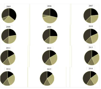
The financial expenditure is divided into four categories, public management expenditure, science and education expenditure, social security expenditure and economic construction expenditure. In case of the annual population differences and in order to reflect the reality of the situation, per capital level to reflect fiscal expenditure situation is applied.

From Figure 1 above, there are four shades from deep to shallow, representing public management expenditure, economic construction expenditure, social se-curity expenditure and the science and education expenditure respectively. The entire circle represents the whole local fiscal expenditure and each part represents the proportion of fiscal expenditure. The 12 figures represent the structure order of fiscal expenditure from 2005 to 2016 respectively; dynamic changes can be seen while observing 12 figures continuously.

(3)

[image:3.595.211.540.60.350.2]

DOI: 10.4236/ojbm.2018.62033 456 Open Journal of Business and Management

[image:3.595.216.540.380.522.2]

Figure 1. The proportion of all kinds of financial expenditure.

Figure 2. Growth rate of various kinds of financial expenditure.

Figure 2 above are four kinds of per capita fiscal expenditure growth rate,

(4)

DOI: 10.4236/ojbm.2018.62033 457 Open Journal of Business and Management It might be due to the acceleration of urban-rural integration process in 2008, breaking the previous discussion in the theoretical stage. The reform of China starts in the rural area, but peaks in cities; the way of prosperity after the first half is not suitable to the reality of urban and rural development. Originally hoping to promote the development of rural areas by urban development, but the reality is that the division of urban and rural and backward rural areas grad-ually becomes obstacles to the further development of the city. A trickledown effect on the backward areas in developed areas has changed into the consump-tion on kinds of rural resources. In view of this, the central government rethinks the development mode of urban and rural areas, implements the rural reform centered on the countryside, and passively forces the initiative for farmers, and speeds up the process of urban-rural integration. As a result, the growth of fiscal expenditure has changed accordingly.

3. Spatial Correlation Standard

There are a lot of spatial correlation standard, Moran index method, Gil coeffi-cient method, local Moran index method, local Gil coefficoeffi-cient method, LM test, LR test, among which the Moran index method, Gil coefficient method can ob-serve the correlation between variables from the whole; local Moran index, local Gil coefficient can gather the detection area; LM test and LR test can further test errors such as the existence of spatial correlation. The research purpose of this part is to test whether there is spatial dependence and fiscal competition among local governments, therefore Moran index, Gil coefficient and local Moran index research are selected.

The Moran’s I index is the first method to be applied to the global cluster test (Cliff and Ord, 1973). It shows that the adjacent areas in the whole study area are similar, different (spatial correlation and negative correlation) are still indepen-dent. Moran’s I index calculation formula is as follows: x

(

)

(

)

(

)(

)

1 1 1 1

2 2

1 1 1 1

n n n n

ij i ij i i

i j i j

n n

ij

ij i i j

i j

n w x x n w x x x x

S w

w x

I

x

= = = ≠

= =

− − −

= =

−

∑ ∑

(1)

The n is the total number of regions in the study; Wij is the spatial weight of the area I and the area J is the adjacent area, which is divided into geographical proximity and economic neighbor. So Wij is divided into geographical weight and economic weight. Xi and XJ are the observation variables of region I and re-gion J respectively, which are the financial expenditure items. X is the average attribute observation variable and S2_{is the variance of observed variables.}

The range of Moran’s I index is generally between −1 to 1; more than 0 says positive correlation; value close to 1 represents that similar values bond together and less than 0 indicates negative correlation values, close to −1 indicates differ-ent attributes bond together. If close to 0, then there is no spatial autocorrela-tion, no spatial dependence, and no expenditure competition.

(5)

DOI: 10.4236/ojbm.2018.62033 458 Open Journal of Business and Management of the product is used in calculation of Moran’s I index, but the Geary index C accounts the deviation between the values. The calculation formula is as follows:

(

)

(

)

(

)

2 1 1

2

1 1 1

1

2

n n

ij i j

i j

n n n

ij i j

i j i

n w x x

C

w x x

= =

= = =

− −

=

−

∑ ∑

∑

(2)

The value of Geary index C is generally between 0 and 2 (2 is not a strict up-per bound), greater than 1 is a negative correlation, equal to 1, indicating no correlation, and less than 1 indicates a positive correlation, contrary to the Mo-ran’s I index.

The local Moran’s I (Anselin, 1995) is used to check whether there are similar or different observation values in the local area. The local Morlan index of area I is used to measure the correlation degree between the area I and its adjacent re-gions. The calculation formula is as follows:

If I is greater than 0, it represents a high value-high value, low value-low value cluster; and if the I is less than 0, the low value-high value, high value-low value cluster is expressed.

4. Spatial Correlation Test

4.1. Data Selection

The article from 2004 to 2016 the provincial dynamic panel data to study from 2005 to 2004 as the base, the relevant financial data in 2016, the main source of “China Statistical Yearbook” and the “statistical yearbook”. Because Chongqing was divided into municipalities in 1997, for the sake of uniformity of the caliber and the length of the dynamic panel data, the last 12 years were selected as the year of analysis.

4.2. Analysis of the Results of Detection Section

[image:5.595.56.539.637.736.2]

4.2.1. Moran Index and Gil Coefficient Detection

Table 1 below is the result of spatial correlation test of national fiscal

expendi-ture in 2016. According to the results, in general, from 2005 to 2016, fiscal penditure spatial correlation index has significant correlation, indicating the ex-istence of spatial dependence of fiscal expenditure in adjacent areas with compe-tition. Specifically, the paper selects two matrixes of geographical weight and economic weight to calculate the spatial dependence of geographically spaced adjacent areas and similar economic regions. Comparing Moran index,

Table 1. Moran’s I index and Geary’s C index test result.

eight 2005 2006 2007 2008 2009 2010 2011 2012 2013 2014 2015 2016 Moran’s I 0.122* 0.15** 0.138* 0.147* 0.169** 0.21** 0.192** 0.202** 0.209** 0.199** 0.175** 0.161** Geographical Geary’s C 0.713** 0.69** 0.719** 0.733** 0.732** 0.713** 0.751** 0.751* 0.745** 0.753* 0.758* 0.768*

(6)

DOI: 10.4236/ojbm.2018.62033 459 Open Journal of Business and Management Moran index of economic weight is more significant than the geographical weight of Moran index, especially in 2005, 2006, 2007 and 2010. The index is more than 0 and close to 1, P values are less than 0.01 which strongly rejects the null hypothesis, therefore, among the total fiscal expenditure competition, eco-nomic space correlation strategy behavior contributes a larger impact on the re-gion. The region selects strategy imitation. Considering Geary s C index, from 2005 to 2016, there is significance, but economic spatial similar regions is more significant than the geographically adjacent areas, indicating that in the total fi-nancial expenditure competition, the area is more affected by economic spatial area. The index is less than 1, indicating that there is a significant positive corre-lation in similar regions. The strategic mimic behavior is selected in the area whose result is consistent with the Moran index.

[image:6.595.64.534.409.737.2]

4.2.2. Local Moran’s I Index Detection

Figure 3 are local Moran’s I index plot of 31 provinces from 2005 to 2016.

Ac-cording to the test results, most of the local governments are in the third qua-drant, namely low value-low value type, indicating that there exists strong de-pendence among adjacent areas, and there is fiscal expenditure behavior. In the figures above, Beijing, Tianjin, Qinghai, Ningxia and Tibet are all in the first quadrant. The first quadrant is high-high value type, indicating that the five local fiscal expenditures are higher than that of other places; the surrounding areas have gathered a higher amount of fiscal expenditure. Beijing and Tianjin

Moran scatterplot (Moran's I = 0.122) C

Wz

z

-1 0 1 2 3 4

-1 0 1 Anhui Henan Jiangx Guangx Sichua Hubei Hunan Guizho Hebei Shando Fujian Gansu Yunnan Shaanx Chongq Hainan Shanxi Heilon Jiangs Jilin Guangd Zhejia Xinjia

NingxiInner Liaoni Qingha

Tianji

Tibet Beijin

Shangh

Moran scatterplot (Moran's I = 0.150) D

Wz

z

-1 0 1 2 3 4

-1 0 1 2 HenanAnhui GuangxJiangx Sichua GuizhoHunan Hebei HubeiShando Yunnan Fujian Gansu Hainan Chongq Shaanx Heilon Jiangs Jilin Guangd Shanxi Zhejia Ningxi Xinjia LiaoniInner Qingha Tianji Tibet Beijin Shangh

Moran scatterplot (Moran's I = 0.138) E

Wz

z

-1 0 1 2 3

-1 0 1 2 HenanAnhui GuangxJiangx Hunan Sichua Hebei

GuizhoHubeiShando Yunnan Fujian Gansu Chongq Shaanx Hainan Shanxi HeilonJilin Guangd Jiangs Zhejia Xinjia

NingxiLiaoni_Inner Qingha

Tianji

Tibet Beijin

Shangh

Moran scatterplot (Moran's I = 0.147) F

Wz

z

-1 0 1 2 3 4

-1 0 1 2 HenanAnhui Hebei

GuangxJiangx_Hunan ShandoHubeiGuizho

(7)

[image:7.595.59.542.64.716.2]

DOI: 10.4236/ojbm.2018.62033 460 Open Journal of Business and Management

Figure 3. Local Moran’s I index test results.

Moran scatterplot (Moran's I = 0.169) G

Wz

z

-1 0 1 2 3 4

-1 0 1 2 Henan Hebei Guangx ShandoHunanAnhuiJiangxHubei

Fujian Guizho Yunnan Guangd Sichua Chongq Shanxi GansuHeilon Shaanx Zhejia JiangsJilin Hainan Liaoni Xinjia Ningxi Inner Qingha Tianji Beijin Shangh Tibet

Moran scatterplot (Moran's I = 0.210) H

Wz

z

-1 0 1 2 3 4

-1 0 1 2 Henan Hebei HunanJiangx ShandoAnhui GuangxHubei Fujian Guizho Yunnan Guangd Sichua Shanxi Gansu Heilon Zhejia Chongq Shaanx JiangsJilin Hainan Liaoni Xinjia Ningxi Inner Tianji Qingha Beijin Shangh Tibet

Moran scatterplot (Moran's I = 0.192) I

Wz

z

-1 0 1 2 3 4

-1 0 1 2 Henan Hebei Shando Hunan Guangx_AnhuiHubei

Jiangx Sichua Fujian Yunnan GuangdGuizho Shanxi Gansu Zhejia Heilon Shaanx Jiangs Jilin ChongqHainan Liaoni Xinjia Ningxi Inner Tianji Beijin Shangh Qingha Tibet

Moran scatterplot (Moran's I = 0.202) J

Wz

z

-1 0 1 2 3 4

-1 0 1 2 Henan Hebei Shando Hunan GuangxHubei Anhui Jiangx Sichua Fujian Guangd Zhejia Shanxi Yunnan Guizho Gansu Heilon Shaanx Jiangs Jilin Hainan Chongq Liaoni Xinjia Ningxi Inner Tianji Shangh Beijin Qingha Tibet

Moran scatterplot (Moran's I = 0.209) K

Wz

z

-1 0 1 2 3 4

-1 0 1 2 Henan Hebei Guangx Shando Hunan AnhuiHubei Sichua Jiangx GuangdFujian Shanxi Zhejia Yunnan Heilon Guizho Gansu Shaanx Jiangs Jilin ChongqHainan Liaoni Xinjia Ningxi Inner Tianji Shangh Beijin Qingha Tibet

Moran scatterplot (Moran's I = 0.199) L

Wz

z

-1 0 1 2 3 4

-1 0 1 2 Hebei Henan Guangx Shando Hunan Anhui Sichua Shanxi Hubei Guangd JiangxFujian Heilon Zhejia Yunnan Gansu Guizho Shaanx Jilin Jiangs Chongq Liaoni Hainan Xinjia Ningxi Inner Tianji Shangh Beijin Qingha Tibet

Moran scatterplot (Moran's I = 0.175) M

Wz

z

-1 0 1 2 3 4

-1 0 1 2 Henan Hebei Shando Hunan Guangx Anhui Sichua Shanxi Jiangx Yunnan Liaoni Fujian Hubei Heilon Guizho Gansu Shaanx Jilin Guangd ZhejiaJiangs Chongq Hainan Xinjia Inner Ningxi Tianji Shangh Qingha Beijin Tibet

Moran scatterplot (Moran's I = 0.161) N

Wz

z

-1 0 1 2 3 4

-1 0 1 2 Henan Hebei Shando Anhui GuangxHunanShanxi

(8)

DOI: 10.4236/ojbm.2018.62033 461 Open Journal of Business and Management are geographically adjacent areas; Qinghai, Ningxia, and Tibet also belong to the adjacent geographical place. However Beijing and Tianjin belong to the Bei-jing-Tianjin-Hebei economic developed areas, while Qinghai, Ningxia and Tibet are economically backward areas. These five areas are similar in total fiscal ex-penditure, indicating that the central government tries to achieve the equaliza-tion of the public level of service through the transfer payment for Qinghai, Ningxia and Tibet. It also can be seen in these three places, besides central gov-ernment related preferential, similar fiscal competition strategies are utilized. The fourth quadrant is high value-low value type, including Shanghai and Inner Mongolia, indicating the existence of spatial heterogeneity in the two regions. Most provinces and cities are located in third quadrant, low value-low value provinces and cities, including Eastern, central and western regions. The fourth part includes Jilin, Gansu, Heilongjiang and Sichuan.

5. Conclusion

The calculation of Moran index, Gil index and local Moran index can draw the conclusion that the total fiscal expenditure of 31 provinces in China has strong spatial dependence, which is not only affected by the geographically adjacent area, but also affected by the economically adjacent area, and the fiscal expendi-ture behavior is competitive.

References

[1] Li, Y. and Shen, K. (2008) Regional Characteristics of Inter District Competition, Strategic Fiscal Policy and FDI Growth Performance. Economic Research, No. 5, 58-69.

[2] Guo, Q. and Jia, J. (2009) Strategic Interaction between Local Governments, Fiscal Expenditure Competition and Regional Economic Growth. Manage the World, No. 10, 17-27 + 187.

[3] Wang, M., Lin, J. and Yu, Z. (2010) The Characteristics of Chinese Local Govern-ment Financial Competition Behavior: Whether “Brother Competition” and “Father Son Dispute” Coexist? Manage the World, No. 3, 22-31 + 187-188.

[4] Lin, J. (2011) The Economic Growth Effect of Local Government Financial Compe-tition in China. Economic Management, 33, 10-15.

[5] Lv, W. and Zheng, S. (2012) Does Fiscal Competition Distort the Structure of Local Government Expenditure?—An Empirical Test Based on the Provincial Panel Data in China. Financial Research, No. 5, 36-40.