Speleothem climate capture of the Neanderthal demise

(1)

Speleothem climate capture of the

Neanderthal demise

Laura Melanie Charlotte Deeprose

BSc (Hons), MSc

June 2018

(2)

(3)

ii

Abstract

The Iberian Peninsula is a region of climatic and archaeological interest as it lies upon

the boundary between the North Atlantic and Mediterranean climatic zones and was

the last refuge of the Neanderthals. The influence of climate changes on Neanderthal

populations remains a mystery due to the lack of independently-dated high-resolution

terrestrial records of past climate and environmental change from the Iberian

Peninsula. The primary aim of this project was to construct a palaeoclimate record

using speleothems from Matienzo, northern Iberia, across the period encapsulating

the Neanderthal demise.

Contemporary cave monitoring of Cueva de las Perlas has demonstrated the potential

for speleothems to be used as indicators of past climate and environmental

conditions. Assessment of cave dynamics through a comprehensive monitoring

programme has classified the karst hydrology, cave ventilation, processes influencing

speleothem growth and proxies preserved within speleothem calcite.

Three speleothems were used to develop records of past climate and environmental

variability between 90,000 and 30,000 years ago. A long-term aridity trend was

evident throughout the record which is interpreted as a response to orbital-forcing.

Sub-orbital climate instability was superimposed onto this long-term trend as

evidenced through wet-dry proxies (δ18_O,_δ13_{C, Mg and Sr). Millennial-scale events}

coincident with the timing of North Atlantic Heinrich Events have been identified and

the sub-orbital climate variability resembles that of North Atlantic

Dansgaard-Oeschger cycles. Therefore, evidence from the speleothems demonstrates a tight

coupling of the North Atlantic Ocean-Atmosphere system throughout MIS3. The Cueva

de las Perlas speleothems have established that the period of the Neanderthal demise

was characterised by climate instability involving abrupt shifts and millennial-scale

events, thereby adding climatic pressures at a time of anatomically modern human

(4)

iii

Declaration

I hereby declare that the work presented in this thesis is my own, except where

acknowledged, and has not been submitted for the award of a higher degree or

other qualification at this or any other institution.

Signed:

Date:

(5)

iv

Acknowledgements

First and foremost, I would like to say a massive thank you to my supervisor Peter

Wynn for his endless support and advice about cave monitoring and speleothem

science. I am also grateful to Phil Barker for his supervisory support and positivity.

Thank you both for your continued enthusiasm throughout the project.

This project would not have been possible without the financial input from the NERC

Envision Doctoral Training Partnership, BGS University Funding Initiative (BUFI) and

NERC Isotope Geoscience Facilities Steering Committee (NIGFSC).

Thank you to the NERC Isotope Geosciences Laboratory (NIGL) team for your analytical

support and advice. I would like to extend a special thank you to Melanie Leng, Andi

Smith, Stephen Noble and Diana Sahy for sharing their knowledge and encouragement

during my visits to Keyworth.

I would like to show my appreciation to those who have provided analytical support

at Lancaster University. To Montse Auladell-Mestre for your support and

encouragement in the earliest stages of laboratory work. To Debbie Hurst and

Catherine Wearing for their technical laboratory assistance. To Dave Hughes for his

extensive commitment to isotope analysis and continuous analytical support. To Andy

Stott and the Centre of Ecology and Hydrology (CEH) for their analytical support

throughout the project. I would like to extend my thanks to Wlodek Tych for his

timeseries expertise and MatLab knowledge and to Gemma Davies for her GIS

support. Additionally, I would like extend my gratitude to Christina Manning for her

analytical support during the trace element analysis and help with the data processing.

A big thank you to the Matienzo caving community who have supported the project

at all stages. A special thanks to Andy Quin for field support and logistics and to Pete

Smith for his continued commitment by visiting the cave monthly throughout the

course of the project. Cave monitoring and speleothem sampling in Cueva de las Perlas

was undertaken with the kind permission from Gobierno de Cantabria, Consejería de

(6)

v

To my fantastic field assistants Joanna Houska for her infectious enthusiasm, Charlotte

Clarke for our hilarious fieldwork shenanigans and to Alex Chapman for his willingness

to come on fieldwork at such short notice!

Throughout my PhD I have met some amazing people and have really grown with them

as we have ventured along this PhD journey together. I would like to say a special

thank you to Ceri Davies and Emma Gray for the endless coffees and chats. To Kirsty

Forber and Rachel Efrat for their emotional support and friendship, frequently over a

burrito or two. To Alistair MacDonald for his sense of humour and encouragement

through our first year at Lancaster. To Rob Larson for his culinary expertise and

willingness to sample the majority Lancaster’s restaurants. Also, a huge thank you to all those who have been a member of the B46 office during my time there, particularly

Ann Kretzschmar, Tamsin Blayney and Runmei Wang along with many others who

have come and gone during the years.

To all those at St. Thomas’ Church Lancaster, Christ Church Alsager and St. Matthew’s Yiewsley who have given me more strength than I could have ever imagined. To my

amazing Heysham life group for your encouragement and for all the discussions we

have shared together.

Without the support of my family and friends this would not have been possible.

Thank you all for your love, support, inspiration and prayers over the past few years.

Your enthusiasm for speleothems has never ceased to amaze me!

And finally, I would like to thank my husband Jonty Warren for his care and passion

for knowledge which has inspired me over the past three and a half years. I will be

(7)

vi

Lists of figures

Figure 2.1: Oxygen isotope records from three Greenland ice cores (Rasmussen et al. 2014)

... 16

Figure 2.2: Marine sediment proxy data from the North Atlantic and the Greenland Ice core record. ... 19

Figure 2.3: Schematic diagram adapted from Fairchild et al. (2006a) ... 27

Figure 3.1: Matienzo maps. ... 64

Figure 3.2: Map of the Matienzo valley. ... 65

Figure 3.3: Images of the hillslope on which Cueva de las Perlas is located. ... 67

Figure 3.4: Cave survey ... 69

Figure 3.5: Photos from Cueva de las Perlas. ... 70

Figure 3.6: Schematic illustrating the basal drilling results from 2015. ... 71

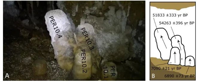
Figure 3.7: PER10.3 and PER10.4 in-situ ... 72

Figure 3.8: PER0 sample from Cueva de las Perlas. ... 73

Figure 3.9: PER10.3 and PER10.4 samples from Cueva de las Perlas. ... 74

Figure 3.10: Soil sampling device. ... 77

Figure 3.11: Diver set-up image and schematic diagram... 79

Figure 3.12: Images of calcite plates in situ. ... 81

Figure 4.1: External hourly and monthly average temperatures... 96

Figure 4.2: Hourly averaged soil temperature. ... 97

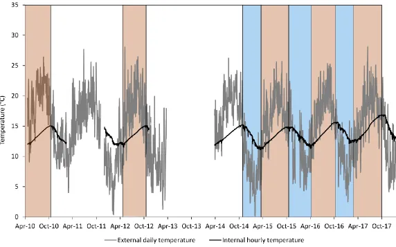
Figure 4.3: External and internal cave temperatures. ... 101

Figure 4.4: Seasonal ventilation phases in temperature. ... 104

Figure 4.5: External pressure. ... 105

Figure 4.6: Cave pressure. ... 106

Figure 4.7: Comparison of internal and external pressure. ... 107

Figure 4.8: External and internal hourly pressure during Jul-15. ... 109

Figure 4.9: CO2 concentrations and carbon isotope values from external air. ... 110

Figure 4.10: CO2 concentrations and carbon isotope values from soil air. ... 111

Figure 4.11: Relationships between soil carbon and temperature. ... 113

Figure 4.12: Hourly and daily cave CO2 concentration (A) and daily variability (B). ... 115

Figure 4.13: Carbon isotope composition of cave air. ... 116

Figure 4.14: Hourly cave CO2 concentrations and external and internal hourly air temperature. ... 117

Figure 4.15: Cave hourly CO2 and internal and external temperatures Jun-17. ... 118

Figure 4.16: Spectral plots for monthly CO2 data. ... 120

Figure 4.17: Spectral analysis case study from Nov-16. ... 121

Figure 4.18: Carbon isotope values for cave air (CA), external air (EA) and soil air (SA) plotted against individual CO2 measurements. ... 122

Figure 4.19: Cave CO2 concentration, cave pressure and external and internal temperature for Jun-17. ... 124

Figure 4.20: Schematic diagram of cave ventilation within Cueva de las Perlas ... 127

Figure 5.1: Matienzo precipitation between Feb-11 to Dec-17. ... 131

Figure 5.2: Water excess, temperature and precipitation amount from Matienzo. ... 132

Figure 5.3: Backward modelled trajectories ... 134

(14)

xiii

Figure 5.5: Rose diagrams illustrating the relative direction of the trajectory analysis (A)

moisture source regions (B) for precipitation events from Sep-15 and Feb-16. ... 136

Figure 5.6: P1, P2 and P3 hourly drips and external precipitation. ... 137

Figure 5.7: External precipitation and P1 drip count between 30/07/17 and 07/12/17... 140

Figure 5.8: Oxygen and deuterium isotope composition of precipitation between Feb-11 and Dec-17. ... 142

Figure 5.9: Precipitation δ18_{O and δD values alongside the GMWL and LMWL.}_{... 143}

Figure 5.10: Precipitation amount and δ18_{Op. ... 144}

Figure 5.11: Temperature and δ18_{Op. ... 144}

Figure 5.12: δ18_{O and}_δ_{D values for the different cave water types. ... 147}

Figure 5.13: δ18_{O and δD values from cave drip waters and seasonal precipitation.}_{... 149}

Figure 5.14: Schematic of karst and cave hydrology from Cueva de las Perlas. ... 150

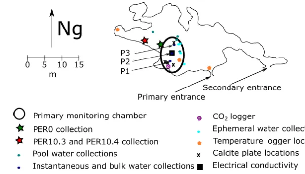
Figure 5.15: Calcite plate locations. ... 152

Figure 5.16: Field photos of calcite plates. ... 153

Figure 5.17: Isotope sampling strategy for calcite plates CP1-16 and CP11. ... 154

Figure 5.18: Variability in δ18_{O values across transects for CP13 and CP1-15 calcite plates. 155} Figure 5.19: Variability in δ18_{O values across transects for CP11, CP1-16 and CP3-16 calcite} plates. ... 157

Figure 5.20: Comparison of modelled (Kim and O’Neil, 1997; Tremaine et al. 2011) and measured oxygen isotope values from calcite plates. ... 160

Figure 5.21: Schematic of the karst hydrological model of Baker and Bradley (2010). ... 164

Figure 5.22: Modelled oxygen isotope values from three hydrological models. ... 167

Figure 5.23: Monthly cave air CO2 (ppm) and drip water PCO2 (ppm). ... 169

Figure 5.24: Relationships between calcite saturation index (SIc) and dripwater PCO2 (A) and SIc and monthly cave air PCO2 (B). ... 170

Figure 5.25: Relationships between instantaneous drip water saturation state, drip water PCO2 and cave air PCO2. ... 171

Figure 5.26: Electrical conductivity spot measurements from instantaneous drips (A), bulk waters (B), pools (C) and ephemeral drips (D). ... 173

Figure 5.27: Electrical conductivity at 25°C for P2 water... 174

Figure 5.28: Electrical conductivity and drip rate. ... 175

Figure 5.29: Hourly CO2 and hourly electrical conductivity from the P2 drip site. ... 176

Figure 5.30: Scatter plot of daily electrical conductivity and daily cave air CO2 ... 177

Figure 5.31: Dripwater electrical conductivity and monitored cave parameters ... 179

Figure 5.32: Carbon isotope composition of bulk cave dripwaters. ... 180

Figure 5:33: Soil temperature, soil CO2 and δ13C values from bulk waters. ... 181

Figure 5.34: Carbon isotope values from bulk water collections. ... 182

Figure 5.35: Carbon isotope values for cave, external and soil air and instantaneous, bulk and pool water plotted against log pCO2. ... 184

Figure 5.36: Trace element concentrations in bulk waters (P1, P2 and P3). ... 189

Figure 5.37: Ca concentration and drip rate for each sample site. ... 191

Figure 5.38: Monthly average drip rate (P1, P2 and P3) plotted against monthly bulk water Ca for the three different drip sites. ... 192

Figure 5.39: Mg/Ca, Sr/Ca and drip rates for P1, P2 and P3 bulk collection sites. ... 194

Figure 5.40: PCP lines for ephemeral, instantaneous, bulk and pool water data ... 196

Figure 5.41: PCP line for Mg/Ca showing P1 instant waters and P1 bulk waters. ... 196

(15)

xiv

Figure 6.1: Age model ‘envelopes’ for the PER10.4 dates produced through COPRA and

OxCal. ... 209

Figure 6.2: Age errors on PER10.4 COPRA and OxCal models. ... 210

Figure 6.3: Proxy comparison of the PER10.4 age models run through COPRA and OxCal. .. 211

Figure 6.5: OxCal modelled age-depth plots for PER10.3 (A) and PER10.4 (B). ... 214

Figure 6.6: Oxygen and carbon isotope profiles for PER0 plotted against depth. ... 215

Figure 6.7: Growth rate for PER0. ... 216

Figure 6.8: Oxygen and carbon isotope profiles for PER10.3 plotted against depth. ... 217

Figure 6.9: PER10.3 growth rate. ... 219

Figure 6.10: Oxygen and carbon isotope profiles for PER10.4 plotted against depth. ... 220

Figure 6.11: PER10.4 growth rate. ... 222

Figure 6.12: δ13_{C values and Mg concentrations for PER10.3 (A) and PER10.4 (B). ... 224}

Figure 6.13: Relationships between Mg and Sr for PER10.3 and PER10.4. ... 226

Figure 6.14: ln(Sr/Ca) and ln(Mg/Ca) plots for Mg vs. Sr for PER10.3 (A) and PER10.4 (B). .. 227

Figure 6.15: Slope values for 500yr time-slices from PER10.3 and PER10.4. Slope values define the relationship between ln(Sr/Ca) and ln(Mg/Ca). ... 229

Figure 6.16: ln(Mg/Ca) and ln(Sr/Ca) values for all of PER10.3 (A) and between 39.1-40ka (B). ... 230

Figure 6.17: ln(Ba/Ca) and ln(Sr/Ca) for PER10.3 between 39.1-40ka. ... 231

Figure 6.18: PER0 oxygen and carbon isotope values and growth rate. ... 233

Figure 6.19: PER10.3 speleothem proxies ... 235

Figure 6.21: Comparison of carbon and oxygen isotope profiles from PER10.3 and PER10.4. ... 239

Figure 6.22: Speleothem palaeoclimate record from Cueva de las Perlas and NH Hemisphere summer insolation at 65°N ... 242

Figure 6.23: Paleoclimate and palaeoenvironmental proxies for PER10.3 and PER10.4 across Perlas event 1. ... 245

Figure 6.24: Paleoclimate and palaeoenvironmental proxies for PER10.3 and PER10.4 across Perlas event 2. ... 247

Figure 6.25: Paleoclimate and palaeoenvironmental proxies for PER10.3 and PER10.4 across event 3. ... 249

Figure 6.26: Identification of three climatic events within the PER10.3 and PER10.4 proxy records. ... 251

Figure 6.27: Averaged 10-yr Mg/Ca from PER10.3. ... 254

Figure 6.28: Averaged 10-yr Mg/Ca from PER10.4 ... 255

Figure 6.29: PER10.3 Mg/Ca data used within the timeseries analysis. ... 258

Figure 6.30: Model constructed for PER10.3 Mg/Ca using 1900-yr and 2000-yr periodicities with the periodicity analysis inset. ... 259

Figure 6.31: PER10.4 Mg/Ca data used within the timeseries analysis. ... 260

... 261

Figure 6.32: Model constructed for PER10.4 Mg/Ca using 1600-yr and 2000-yr periodicities with the periodicity analysis inset. ... 261

Figure 7.1: Comparison of palaeoclimate records from across the North Atlantic region. ... 274

Figure 7.2: Comparison of Cueva de las Perlas speleothem Mg/Ca to ice core data. ... 277

Figure 7.3: Comparison of Cueva de las Perlas speleothem Mg/Ca to ice core and marine pollen data. ... 278

(16)

xv

List of tables

Table 2.1: Onset ages for MIS5-2 (as defined by Lisiecki and Raymo, 2005). ... 13

Table 2.2: A summary of the different drip regmines in Crag Cave (Baldini et al., 2006). ... 33

Table 3.1: Cation standard information. ... 84

Table 3.2: Anion standard information ... 84

Table 3.3: Standard deviations for different standards used in the equilibration method. .... 85

Table 3.4: Standard values and precisions for oxygen and deuterium stable isotope analyses. ... 86

Table 3.5: Standard deviations and limits of detection for ICP-OES analysis of rock powders in solution. ... 91

Table 3.6. Summary of laboratory methods. ... 93

Table 4.1: Lag times between maximum external temperatures and maximum soil temperatures. ... 98

Table 4.2: Annual average temperatures and standard deviations from the monitoring chamber and external environment. ... 100

Table 4.3: Summary of soil air carbon isotope values. ... 111

Table 4.4: Carbon isotope values from soil organic matter. ... 112

Table 4.5: Carbon isotope values from rock samples. ... 114

Table 4.6: Annual and seasonal CO2 concentrations. ... 114

Table 5.1: Average annual hourly drip rate for P2. ... 138

Table 5.2: Average isotopic values for different dripwater types. ... 146

Table 5.4: Oxygen and carbon isotope composition of calcite plates. ... 154

Table 5.5: Summary of transect indicators of equilibrium deposition (δ18_{O average, standard} deviation, R2 between δ18_{O and δ}13_{C values and within transect range) for CP13 and CP1-15} calcite plates. ... 156

Table 5.6: Summary of transect indicators of equilibrium deposition (δ18_{O average, standard} deviation, R2 between δ18_{O and δ}13_{C values and within transect range) for CP11, CP1-16 and} CP3-16 calcite plates. ... 158

Table 5.7: Summary of indicators of equilibrium deposition (δ18_{O average, standard} deviation, R2 between δ18_{O and δ}13_{C values and within transect range) for CP1 W-16, CP3} S-16 and CP3 W-S-16 calcite plates. ... 158

Table 5.8: Determination of isotopic equilibrium using calcite plates. ... 161

Table 5.9: Parameters used within the hydrological models... 165

Table 5.10: Average instantaneous and bulk carbon isotope values for the different drip sites. ... 183

Table 5.11: Average rainwater and cave water trace element concentrations. ... 185

Table 5.12: Trace element concentrations for bedrock samples. ... 186

Table 6.1: U-Th sample data for PER0, PER10.3 and PER10.4. ... 203

Table 6.2: Parameters used in OxCal age models for PER0, PER10.3 and PER10.4. ... 212

Table 6.3: Summarised trace element data for PER10.3. ... 218

Table 6.4: Summarised trace element data for PER10.4. ... 221

Table 6.5: Summary of proxy shifts in the PER10.3 record. ... 234

Table 6.6: Summary of proxy shifts in the PER10.4 record. ... 236

Table 6.7: Timings of isotopic shifts in PER10.3 and PER10.4. ... 238

(17)

1

1. Introduction

Between 90,000 – 30,000 years before present (BP) the North Atlantic region was subject to dramatic oscillations in climate and environment (Bond et al., 1993; Rasmussen et al., 2014). This time period encapsulates the Neanderthal population decline and eventual extinction. The demise of the Neanderthals has been attributed

at least in part to changes in climate, with the Iberian Peninsula acting as the last

refuge of the Neanderthals (d’Errico and Sánchez Goñi, 2003; Finlayson and Carrion, 2007; Tzedakis et al., 2007; Wolf et al., 2018). In order to attribute the influence of climate change on Neanderthal populations, long-term high-resolution records of past

climate variability are required. Although numerous marine records from the North

Atlantic have been used to determine past environmental variability (Roucoux et al.,

2005; Sánchez Goñi et al., 2008, 2018), there remains a lack of high-resolution independently dated terrestrial climate records from the Iberian Peninsula.

The Iberian Peninsula lies upon the boundary between two climatic zones: the North

Atlantic and the Mediterranean. Consequently, the region is highly sensitive to short-

and long-term variations in atmospheric circulation (Martín-Chivelet et al., 2011). Evidence from a variety of proxy archives has demonstrated a tight coupling of the

North Atlantic Ocean-Atmosphere system throughout MIS3 and variations in

atmospheric and oceanic conditions have been identified as driving mechanisms

behind widespread abrupt millennial-scale variability (Bond et al., 1993; Rasmussen et al., 1996; Roucoux et al., 2005). The sensitivity of the Iberian Peninsula to variations in climate demonstrates the potential of the region to provide long-term

palaeoclimate records.

Speleothems are becoming increasingly utilised as valuable terrestrial archives of

palaeoclimate and palaeoenvironment. Calcareous speleothems preserve a record of

climatic and environmental conditions through incorporation of stable isotopes and

trace elements into the calcite crystal lattice (McDermott, 2004, Fairchild and Baker,

2012). The chemical signal preserved within speleothem calcite can be influenced by

the atmosphere, soil, vegetation, karst and cave system. Therefore, variability in

(18)

2

(Fairchild and Baker, 2012). A key advantage to speleothem records is their ability to

be independently dated through uranium-series methods (McDermott, 2004; Fairchild

and Baker, 2012).

Prior to speleothem analysis, cave systems must be understood as each cave system

is unique and will behave individually. Hydrological routing through the karst

(Miorandi et al., 2010; Bradley et al., 2010; Baker and Bradley, 2010), karst-water interactions (Fairchild et al., 2000; Fairchild and McMillan, 2007) and cave ventilation (Spӧtl et al., 2005; Mattey et al., 2010; James et al., 2015; Smith et al., 2015) can influence chemical signatures in speleothem calcite. Understanding cave

environments in which speleothems are depositing is critical in order to accurately

interpret geochemical signals in speleothems in relation to climate and environmental

variability.

This thesis will present a cave monitoring study and subsequent speleothem

reconstruction from Cueva de las Perlas, Northern Spain. The primary aim of the

project is to reconstruct palaeoclimate from Matienzo (Northern Iberia) during the

period of the Neanderthal Demise; which in this study will encompass 90,000-30,000

years BP. This aim can be broken down into two sub-aims:

1. Understand the internal cave dynamics of Cueva de las Perlas

2. Collect and produce a climatic record from Cueva de las Perlas

An extensive cave monitoring programme has been undertaken within Cueva de las

Perlas to determine how the external climate signal is transferred into the speleothem

calcite and provide insight into the various processes which may act to modify the

climate and environmental signal. The results and discussion of the cave monitoring

programme are presented in chapters 4 (cave air characteristics) and 5 (drip water

chemistry).

Dating of the selected speleothems from Cueva de las Perlas was undertaken to

determine periods of growth and identify speleothems suited to the present study.

Further uranium-series dating of these speleothems was used to produce an

(19)

3

produce records of past climate and environmental change through stable isotope and

trace element analyses and the results are presented in chapter 6.

The speleothem records from Matienzo have been compared to others across the

North Atlantic region in order to determine whether any detected shifts in climate and

environment are apparent only at a local scale or can be linked to other records from

the wider region (chapter 7). The impact of changes in climate and environment on

(20)

4

2. Literature review

The primary aim of this project was to reconstruct climate and environmental

variability during the period of the Neanderthal demise. This literature review will

therefore discuss the key topics of Neanderthals, climate change and cave monitoring

in order to meet the primary aim. This chapter will first introduce possible mechanisms

for the Neanderthal extinction and highlight the complexities involved in dating the

timing of the Neanderthal demise. A primary theory invokes climate change as the

mechanism driving the extinction of Neanderthal populations and section 2.2 will

provide an overview of climate and environmental variability between 90-25ka which

encapsulates the Neanderthal population decline and extinction. Caves hold clues to

reconstructing the environment and landscapes in which the Neanderthals were living

and section 2.3 will discuss how speleothems can be used as archives for

palaeoclimate and palaeoenvironmental reconstruction. In order to interpret

speleothem records accurately it is important to understand the cave system in which

they are growing and section 2.4 will present an overview of cave monitoring and its

significance. Section 2.5 will discuss speleothem growth whilst the final section (2.6)

will discuss speleothem geochemistry with respect to stable isotope analyses, trace

element composition and dating through U-series.

2.1 The Neanderthal demise

2.1.1 Overview

The Neanderthals, Homo neanderthalensis, were a hominin species found throughout Eurasia between 300-30ka BP (Harvati, 2010). The reasons why the Neanderthals went

extinct have long fascinated scientists, however even today it is not fully understood

why this species disappeared. Two key hypotheses have emerged; the first proposes

(21)

5

will explore the key points of each argument, particularly in light of recent dating

which has challenged the exact timing of the Neanderthal disappearance (Higham et al., 2011, 2014).

The replacement of Neanderthals by Anatomically Modern Humans is complex and

diachronous across Europe. The scarcity of fossil remains hinders understanding of

this transition which is primarily identified through the succession of stone tool

assemblages (Hoffecker, 2009; Hublin, 2015; Staubwasser et al., 2018). The Middle-Upper Palaeolithic Transition is characterised by a shift from Mousterian technologies

associated with Neanderthals to Aurignacian technologies associated with modern

humans and often “transitional” technologies will be associated with specific regions (Staubwasser et al., 2018). The Châtelperronian technology is an example of a transitional technology which has been associated with Neanderthals (Bailey and

Hublin, 2006). Key archaeological sites from the northwestern Iberian Peninsula which

have recently been re-dated by Higham et al. (2014) include: La Viña, El Sidrón, La Güelga, Esquilleu, Morín, Arrillor, Labeko Koba, Lezetxiki. Within the Matienzo

depression, Cueva de Cofresnedo is a site of archaeological interest. An Aurignacian

layer has been dated to 31,360yr BP and this most likely overlies sediments associated

with the Mousterian (Smith, 2006).

2.1.2 Climate

2.1.2.1 Climatic variability

Orbitally-forced climate changes throughout the Late Pleistocene have been proposed

as the driving mechanism for the migration of H. sapiens out of Africa (Timmerman and Friedrich, 2016; de Menocal and Stringer, 2016) strengthening the argument for

a dynamic relationship between hominin migration and climate change. Although the

evidence for this hypothesis is not empirical, such long-term changes in climate may

have influenced Neanderthal populations or potentially it was the unprecedented

climatic variability during Marine Isotope Stage 3 (MIS3) which triggered the

Neanderthal demise. MIS3 encompasses the period between 57-29ka and is

(22)

6

warming events known as Dansgaard-Oeschger (DO) events within MIS3 and these are

expressed as abrupt shifts from stadial climatic conditions to milder interstadial

climatic conditions, followed by a gradual return to colder stadial conditions

(Dansgaard et al., 1993). Another key feature of MIS3 is the presence of Heinrich events which are periods marked by significantly reduced sea surface temperatures

and large releases of icebergs from the Laurentide ice sheet. Each Heinrich event

marks the coldest period of a DO event and is followed by a rapid increase in

temperature (Bond et al., 1993). Further information about Heinrich events and DO variability can be found in section 2.2.

Recent work by Staubwasser et al. (2018) has shown archaeological sterile layers coincide with Greenland Stadial 12 (GS12), GS11 and GS10. These periods document

cold and arid conditions at the time of the transition between Neanderthals and

Anatomically Modern Humans. Additionally, the study highlights the diachronous

nature of the Middle-Upper Palaeolithic Transition across Europe.

It has been suggested that climatic variability can place a significant amount of stress

on mammalian populations (Barnosky et al., 2004) and various authors have proposed the Neanderthals became extinct in relation to climatic instability during MIS3

(Finlayson and Carrion, 2007; Tzedakis et al., 2007). Stewart (2005; 2007) has proposed that the Neanderthal extinction should be included in the wider Late

Pleistocene extinction of the megafauna related to climatic deterioration during MIS3

towards the Last Glacial Maximum (LGM). These papers have identified the

Neanderthals as part of a non-analogue environment incorporating a mixture of

boreal, steppic and temperate faunas and environments. A fall in temperatures and

carrying capacity of the landscape due to climatic deterioration towards the LGM has

been determined by Stewart (2005) to have led to the spread of AMH, a fall in the

number of carnivore numbers on the landscape including the cave bear, extinction of

numerous animals including the mammoth, straight-tusked elephant, the Merck’s rhinoceros and crucially the demise of the Neanderthals. Additionally, other authors

have highlighted the importance of the non-analogue environment which was home

to the Neanderthals and the vulnerability of such landscapes to the climatic instability

(23)

7

MIS3 the shift towards cooler and drier conditions, especially during Heinrich events

and towards the LGM, may have led to shifts in vegetation communities and

extinctions of specific taxa (Burjachs et al., 2012). It was these changes, combined with an increase in habitat fragmentation also related to climatic deterioration (Magniez

and Boulbes, 2014) which may have placed Neanderthal populations under increased

environmental stress and later contributed to their demise.

2.1.2.2 Heinrich events

Heinrich events are evident in a variety of records from across Europe, particularly the

Iberian Peninsula. These events appear to cause an overall reduction in temperature

and an increase in aridity in these regions. Stalagmites from Villars Cave, SW France

(Wainer et al., 2009; Genty et al., 2010) and Sofular Cave, NW Turkey (Fleitmann et al., 2009) have used stable isotope variations to identify Heinrich events 4 (H4) and 5 (H5) as periods of increased aridity and cooling. Evidence from a variety of marine

cores from the Iberian margin (Roucoux et al., 2005; Salgueiro et al., 2010) have used various different proxies including pollen, stable isotopes and planktonic foraminifera

identification to demonstrate periods of climate cooling across the North Atlantic. The

marine cores from this region have identified the Heinrich events as periods of

reduced sea surface temperatures. Additionally, Roucoux et al. (2005) indicated shifts in land pollen associated with Heinrich events, particularly a decrease in Pinus related to H4, implying dry and cooler conditions during the H4 event. Finally, lake records

from Western Europe have shown through geochemical analysis and pollen

identification, that Heinrich events are represented by cool temperatures and

increased aridity on land. For example, at Fuentillejo maar, Spain, cold and arid

conditions are thought to have dominated H4 due to lower lake levels, reduced total

organic carbon and an increase in Juniperus and steppic-vegetation (Vegas et al.,

2010). Additionally, the lake record from Les Echets, France exhibits a hiatus around

the timing of H4, suggesting a cold and dry period (Veres et al., 2009).

2.1.2.3 H4

In the past, studies have often linked the disappearance of Neanderthals with the

dramatically reduced temperatures and enhanced aridity which spread across Europe

(24)

8

cooler and more arid conditions which saw the expansion of semi-desert vegetation

in the western Mediterranean and the expansion of grasslands in the North (Sánchez

Goñi et al., 2008). Adaptation to the severe extremes of H4 would have forced changes in Neanderthal subsistence strategies and ability to cope with severe winters, and

perhaps the Neanderthals could not adapt to these abrupt changes. AMH on the other

hand appear to have had several prior adaptations such as complex tools and a social

capacity which may have given them an advantage over Neanderthal groups (Mellars,

1998).

Alternative theories have argued for H4 leading to a later extinction of Neanderthals

in southern Iberia associated with the expansion of semi-desert in this region (d’Errico and Sánchez Goñi, 2003; Sepulchre et al., 2007). It is argued that aridification associated with H4 prevented the migration of AMH into southern Iberia until after

H4. Model simulations have estimated a maximum vegetation of just 25% combined

with a vast expansion of semi-desert environments across Iberia during H4 (Sepulchre

et al., 2007) and pollen evidence has justified this model (d’Errico and Sánchez Goñi, 2003). The enhanced aridity across central and southern Europe has led to the

proposal that Neanderthal populations declined in density during this period due to a

reduction in ungulate biomass (Sepulchre et al., 2007). However, in spite of the population decrease during H4, the spread of semi-desert environments appears to

have allowed the Neanderthals to occupy southern Iberia by slowing the advance of

AMH (d’Errico and Sánchez Goñi, 2003).

The Campanian Ignimbrite (CI) eruption at 40ka is known as one of the most explosive

events in Europe and its impact on the Neanderthals has also been debated (Fedele et al., 2008; Lowe et al., 2012). The volcanic event is proposed to have significantly impacted the ecology of the Mediterranean region and caused a ‘volcanic winter’ coincident with the onset of the H4 event resulting in widespread and rapid cooling

(Fedele et al., 2008). These factors may have impacted Neanderthal populations by causing them to contract or by leading to evolutionary and cultural development in

(25)

9

Although, the authors do specify the immediate impact of climatic cooling as a

consequence of the eruption would have had a significant influence on Neanderthal

lifestyles and survival (Black et al., 2015). Additionally, recent work by Davies et al.

(2015) presented strengthened chronological frameworks to investigate the response

of Neanderthal and AMH populations to abrupt climate shifts and environmental

disasters. The paper concluded that it remains difficult to attribute the Neanderthal

demise to a specific abrupt environmental transition or an environmental disaster

such as the Campanian Ignimbrite.

2.1.2.4 Recent re-dating

Significant improvements to the radiocarbon dating technique have recently revised

interpretation of the Neanderthal extinction (Higham et al., 2014; Wood et al., 2014). These improvements include: the selection of more material for dating e.g. bone and

artefacts, more effective removal of contamination and an extended calibration curve

covering the past 50ka (Davies, 2014). Sites from across Eurasia have been re-dated

and calibrated using Bayesian age modelling and the results have indicated the

disappearance of the Mousterian culture associated with the Neanderthals at around

42ka BP (Higham et al., 2014; Wood et al., 2014).

2.1.2.5 H5

In light of recent re-dating some authors have begun to identify H5 as a key factor

which led to the extinction of the Neanderthals (Galvan et al., 2014; Garralda et al.,

2014). The study by Galvan et al. (2014) dated and analysed the archaeological sequence at El Salt, Spain and found that the site was occupied by Neanderthals until

~45ka. Importantly, at ~45ka there was evidence of increased aridity and grassland

expansion related to the H5 event and at El Salt this climatic event is associated with

the last presence of the Neanderthals. Teeth from El Salt have been studied and

represent the last occupation of the site between 47.2±4.4 and 45.2±3.4ka. The

overlying unit which does not contain any archaeology, represents abandonment of

the site potentially due to a climatic shift to arid conditions as shown through the

sediments (Garralda et al., 2014; Galvan et al., 2014).

(26)

10

abandonment of Neanderthal sites across Europe which allowed AMH to colonise and

spread into the abandoned eastern Mediterranean, after H5. Müller et al. (2011) argued that the shift from desert-steppe to open forest associated with the climatic

amelioration after H5, as shown by pollen records from Tenaghi Philipon, NE Greece,

permitted the rapid spread of AMH into and across Europe before the Neanderthals

could reoccupy this region.

2.1.3 Competition with AMH

2.1.3.1 Extinction through competitive exclusion

The role of AMH in the Neanderthal extinction has led to extensive debates. The model

of Banks et al. (2008) combined palaeoclimate data with archaeological and chronological data and the results have suggested that Neanderthals contracted their

range during Greenland Interstadial 8 following H4 due to the expansion of AMH and

any climatic causes can be rejected. The use of cryptotephra as an isochronous marker

horizon has argued the technological transition between the Middle and Upper

Palaeolithic occurred prior to the H4 event and the Campanian Ignimbrite eruption

(Lowe et al., 2012). Therefore, the authors have suggested competition with AMH was the driving factor leading to the Neanderthal demise.

D’Errico and Sánchez Goñi (2003) have argued for a combined influence of both AMH competition and climate change. The authors have suggested the climatic

amelioration after H4 led to the expansion of AMH across the Iberian Peninsula and

the arrival of AMH in the southern Iberian Peninsula and associated competition

ultimately resulted in the extinction of the Neanderthals (d’Errico and Sánchez Goñi, 2003). Additionally, Müller et al. (2011) argued that a combination of the severe climatic conditions associated with H5 combined with increased competition with

AMH led to the demise of the Neanderthals.

2.1.3.2 Problems with dating

The key problem for determining the causes of the Neanderthal extinction is dating.

As shown in section 2.1.2.4, recent dating has changed our view of when the

(27)

11

AMH in Europe with key findings from Kent’s Cavern, UK, dated to 44.2-41.5ka (Higham et al., 2011) and Grotta del Cavallo, Italy, dated to 45-43ka (Benazzi et al.,

2011). The earlier arrival of AMH complicates the causes for Neanderthal extinction as

the two species may have overlapped in areas of Europe. Recent work by Higham et al. (2014) has identified a potential overlap between Neanderthals and AMH of 2,600-5,400yrs, which is enough time for cultural and genetic overlap between the two

species.

2.1.4 Genetic evidence

In recent years, technological advances have allowed improved and detailed

understanding of Neanderthal genetics (Green et al., 2010). Genetic evidence has identified Neanderthal populations were small and isolated which led to inbreeding

(Castellano et al., 2014; Prüfer et al., 2014). The pro-longed population bottle-neck as a consequence of inbreeding reduced the genetic diversity of the Neanderthal

population (Prüfer et al., 2014). Subsequently, Neanderthals were 40% less fit than the AMH who were migrating across Eurasia (Harris and Nielsen 2016; 2017). If the

fitness disadvantage was passed down to Neanderthal-AMH hybrid offspring,

Neanderthal genes are proposed to be selected against leading to a reduction in

Neanderthal ancestry over time as a consequence of natural selection (Juric et al.,

2016; Harris and Nielsen, 2016; 2017). Genetic evidence may therefore imply

Neanderthals did not truly become extinct but were assimilated into the genomes of

AMH (Harris and Nielsen, 2017).

On the other hand, genetic evidence has led some authors to link population

bottlenecks and extinction of Neanderthals with climate changes. Analysis of recent

western Neanderthal mtDNA, i.e. the mitochondrial DNA of Neanderthals present in

Western Europe since 48ka, has revealed a reduced amount of genetic variation when

compared to eastern and older Neanderthals (Dalén et al., 2012). The paper has proposed the genetic turnover in recent western Neanderthals was most likely a result

of the climatic variability during MIS3. The authors speculate North Atlantic cold

periods associated with H5 and H6 influenced the terrestrial environment which led

(28)

12

2.1.5 Summary

It is apparent that the demise of the Neanderthals is a complicated issue and the

numerous factors which may have been responsible are still debated. Primary

problems include dating issues in addition to the sparse resolution of the

archaeological record and the diachronous nature of the transition between

Neanderthals and AMH. Important to this project is the role of climate but as d’Errico and Sánchez Goñi (2003) pointed out, there remains a lack of high resolution,

independently dated and continuous palaeoclimate records from the Iberian

Peninsula and this remains true today. Therefore, there is a need to create such

records from across the Iberian Peninsula before the role of climate change in the

Neanderthal extinction can be addressed.

2.2 Climate change 90-25ka

2.2.1 Introduction

Recent improvements in the independent dating of ice core, marine and terrestrial

records have permitted the correlation of these records across the globe and in

particular the northern hemisphere. The correlation of these various records has

begun to identify leads and lags in the climate system as well as enhancing current

understanding of the forcing factors behind these abrupt changes (Blockley et al.,

2012). Between 90-25ka the climate of the North Atlantic was influenced by orbital

forcing but it was also driven by sub-orbital mechanisms. Evidence from different

archives from across the northern hemisphere will be presented in this section as well

as a summary of the forcing mechanisms.

2.2.2 Orbitally-driven climate change

Orbital forcing was long hypothesised to influence the Earth’s climate (Croll, 1864; Milankovitch, 1941) and support for the orbital forcing theory later came from the

oxygen isotope records of planktonic foraminifera preserved within marine sediments

(29)

13

foraminifera within deep-sea cores were identified as a proxy for global ice volume

(Shackleton, 1967). This finding led to the development of the SPECMAP astronomical

timescale which tuned stacked oxygen isotope records from planktonic foraminifera

to orbital forcing, producing a single global marine δ18_{O record (Imbrie}_{et al.,}_1984;

Martinson et al., 1987). The development of the SPECMAP timescale permitted comparison of marine δ18_{O records with other proxies from around the world and}

contributed to understanding climatic processes which operate over

Glacial-Interglacial timescales (Bassinot, 2009). The development of the LR04 stack increased

the resolution of the SPECMAP timescale and extended it back to 5.3Myr (Lisiecki and

Raymo, 2005). It is important to note that there are issues associated with tuning any

record to orbital forcing (Blaauw, 2012) and recent work has also highlighted the

chronological limitations associated with marine cores (Austin and Hibbert, 2012).

Nevertheless, these long records of changes in the δ18_{O composition of foraminifera}

led to the definition of Marine Isotope Stages (MIS) which correspond to

Glacial-Interglacial cycles driven by orbital forcing (Imbrie et al., 1984; Martinson et al., 1987; Lisiecki and Raymo, 2005).

Ages for the onsets of different marine isotope stages relevant to this study are shown

in table 2.1. Glacial marine isotope stages are represented by even numbers whilst

Interglacial marine isotope stages are represented by odd numbers. However, MIS3 is

an anomaly as it is characterised by a high degree of climate instability in comparison

to the relatively stable glacial conditions of MIS 4 and MIS2 (Bond et al., 1993; Shackleton et al., 2000; Lisiecki and Raymo, 2005).

Table 2.1: Onset ages for MIS5-2 (as defined by Lisiecki and Raymo, 2005).

Marine Isotope Stage Onset age (ka)

MIS2 29

MIS3 57

MIS4 71

MIS5 130

Marine sediment cores spanning MIS3 have identified a period of terrestrial tree

(30)

14

Schӧnfeld et al., 2003; Roucoux et al., 2005). It has been argued that these proxies indicate a long-term aridity and cooling trend throughout MIS3 on the Iberian

Peninsula and this period corresponds to a reduction in Northern Hemisphere

Summer Insolation.

2.2.3 Sub-orbital climate variability

2.2.3.1 Ice cores

The identification of abrupt millennial-scale climatic events in the Greenland ice cores

(Dansgaard et al., 1993; Grootes et al., 1993) has led to numerous studies which have focussed on identifying these climatic patterns in terrestrial and marine records

(Voelker, 2002).

Ice core records from Greenland have demonstrated an unstable climate dominated

the Last Glacial Period, characterised by a sequence of abrupt climatic shifts known as

Dansgaard-Oeschger (DO) events. During DO events climate abruptly switched from

cold conditions to mild interstadial conditions (Dansgaard et al., 1993; Johnsen et al.,

1992; Rasmussen et al., 2014). The chronology of the DO events is represented in Greenland by Greenland Interstadials (GI) and Greenland Stadials (GS) with GI periods

defined by warm conditions and GS periods defined by cold conditions (figure 2.1)

(Rasmussen et al., 2014). Across the Last Glacial Cycle 25 DO events (GI periods) have been identified and are defined by a sharp increase in temperature followed by a

gradual return to stadial conditions (GS periods) (NGRIPmembers, 2004; Kindler et al.,

2014; Rasmussen et al., 2014). The temperature increase associated with the DO events varies between 5°C to 16.5°C (Kindler et al., 2014).

The chronology of these events (GI and GS) has recently been redefined through

comparison of the oxygen isotope compositions and calcium ion concentrations in

three ice-core records (NGRIP, GRIP, GISP2) from Greenland on the same timescale.

The time period examined herein (90-25ka) spans GI-22 to GS-3. It is evident from the

Greenland ice core records that the period between 90-25ka, similar to the rest of the

Last Glacial Period, was characterised by rapid increases in temperature at the onset

(31)

15

(32)

[image:32.842.79.777.118.348.2]

Figure 2.1: Oxygen isotope records from three Greenland ice cores (Rasmussen et al. 2014) using the chronological framework developed by Seierstad et al. (2014). Numbers express Greenland Interstadial onsets as defined by Rasmussen et al. (2014). Data available from: http://www.iceandclimate.nbi.ku.dk/data/

(33)

17

2.2.3.2 Marine

Evidence from a series of marine cores from the North Atlantic demonstrated a

pattern of millennial-scale abrupt increases in temperature followed by gradual

cooling, similar to the DO cycles in Greenland (Bond et al., 1993). A key finding of Bond

et al. (1993) was the identification of a series of ‘saw-toothed’ cooling cycles (now known as Bond cycles) composed of numerous DO cycles, gradually becoming colder

and culminating in a Heinrich event. The Heinrich events mark the coldest point of a

Bond cycle where large numbers of icebergs were released into the North Atlantic

(Bond et al., 1993). Heinrich events 5, 4 and 3 occurred during the time period studied in this thesis (86-27ka) with dates of 45,000, 38,000 and 31,000 respectively

(Hemming, 2004).

Evidence from marine records across Europe express similar climatic variability during

MIS3. For example marine core MD99-2281 from south of the Faroe Islands expressed

climatic instability throughout MIS3 as a result of the dynamic behaviour of the

European ice sheets during this time (Zumaque et al., 2012). The multi-proxy record studied by Zumaque et al. (2012) identified a series of oscillations matching the GI and GS events; GI events were milder while stronger ice sheet calving occurred during GS

events. Comparably, the Eastern Mediterranean pollen records from marine core

9509 have indicated a reduction in forests and an increase in arid herbaceous flora

between 43.5-16.2ka (Langgut et al., 2011). Furthermore, Heinrich events 6-2 have been identified in marine core 9509 based upon short-lived reductions in arboreal

vegetation suggestive of a decline in moisture availability and thus Langgut et al.

(2011) have demonstrated the expression of North Atlantic climate events in the

Eastern Mediterranean.

Marine core MD95-2042, taken from off the coast of the Iberian Peninsula, has

demonstrated through planktonic δ18_{O analyses, stadial-interstadial climate variability}

correlating with DO cyclicity in Greenland (Shackleton et al., 2000). Further work on MD95-2042 by Sánchez Goñi et al. (2000) identified a pattern of DO cycles and Heinrich events through a combination of dinocyst, pollen, foraminifera and coarse

lithic analyses as well as the δ18_{O profile. The study demonstrated a three-phase}

(34)

18

and dry conditions. In contrast, the first and final phases exhibited milder and more

humid climates. The pollen record from MD95-2042 highlighted several periods

corresponding to DO stadials characterised by steppic taxa such as Artemisia and Chenopodiaceae (Sánchez Goñi et al., 2000). However, caution should be applied when trying to link these events in southwest Europe to DO cyclicity in the Greenland

ice cores, as the MD95-2042 record has been tied to the GISP2 timescale on the basis

that rapid warming was synchronous between the two regions (Sánchez Goñi et al.,

2000, Shackleton et al., 2000).

However, despite the dating issues and alternative influences, numerous cores from

around the Iberian Peninsula have shown a similar pattern of DO cyclicity and Heinrich

events. Sánchez Goñi et al. (2018) discuss the significant contribution of pollen studies in the identification of DO variability and Heinrich events on the Iberian Peninsula. A

pollen record from the Alboran Sea (MD95-2043) showed an alternation between

semi-desert vegetation such as Artemisia and Chenopodiaceae during stadials and Heinrich events and mixed oak forest during interstadials (Fletcher and Sánchez Goñi,

2008). Two cores off the Iberian margin have demonstrated variations in productivity

are coincident with DO variability and Heinrich events (Pailler and Bard, 2002). The

combined pollen and planktonic δ18_{O data from marine core MD95-2039 has provided}

evidence for millennial-scale variability. Fluctuations in thermophilous tree

populations correspond to shifts in SSTs with warmer SST synchronous with expanding

thermophilous tree populations (Roucoux et al., 2005). In addition, Heinrich events in the Roucoux et al. (2005) study are demonstrated to have been more severe than DO stadials due to the greater reduction in Pinus. Interestingly, the fire regime of western France has been shown in marine core MD04-2845 to exhibit DO variability and

Heinrich events through multiproxy analysis of microcharcoal, pollen and organic

carbon in conjunction with analysis of ice rafted debris and isotopic analyses of

(35)

19

(36)

20

2.2.3.3 Speleothems

Evidence for climatic instability during MIS3 has been shown from oxygen and carbon

stable isotope records from speleothems across Europe (Spötl and Mangini, 2002;

Genty et al., 2003; Wainer et al., 2009; Fleitmann et al., 2009; Genty et al., 2010; Moseley et al., 2014). Stalagmites from Hölloch Cave, northern Alps, exhibited millennial-scale increases in δ18_{O values}_{of up to 3‰ which were correlated to DO}

events in the Greenland ice cores, higher sea surface temperatures in the NE Atlantic

Ocean and strengthening of the East Asian Summer Monsoon across Asia (Moseley et al., 2014). A similar correlation was found in the oxygen isotope profile from Solfular Cave, Turkey (Fleitmann et al., 2009). Additionally, carbon isotope records have been used to infer climate changes across MIS3 from speleothem records with shifts in δ13_C

values reflecting varying vegetation cover and soil microbial activity directly related to

temperature and precipitation (Wainer et al., 2009, Fleitmann et al., 2009, Genty et al., 2003, Genty et al., 2010). During periods of climatic amelioration microbial activity in the soil zone increases, as does the amount of overlying vegetation and as a result

the δ13_{C values in the soil become lowered (Wainer}_{et al.,}_{2009). Carbon and oxygen}

profiles from terrestrial speleothems have therefore provided crucial evidence for the

response of these areas to North Atlantic climate events and have identified key leads

and lags within the climate system. For example, Moseley et al. (2014) demonstrated that the DO events in the Greenland ice cores lagged the large amplitude

millennial-scale increases in δ18_{O values preserved within stalagmites from Hölloch Cave.}

Throughout MIS4-2, speleothem growth was rare in NW Spain as a result of reductions

in temperature and humidity (Stoll et al., 2013). Sporadic periods of growth in MIS3 appear to coincide with warmer SST (>13.7°C) associated with DO interstadials.

2.2.3.4 Lacustrine

Lake records which have been precisely and accurately dated through a combination

of radiocarbon dating, tephrochronology and varve counting, can provide important

terrestrial archives of palaeoenvironment (Hayashi et al., 2010; Nakagawa et al.,

2012). The Les Echets palaeolake, eastern France has provided a vital record of

(37)

21

2008). Studies from Les Echets have revealed a similar pattern of stadial-interstadial

climate variability during MIS3 as well as the identification of Heinrich events 4, 3 and

2, similar to those recorded in marine and ice core records. Interstadial periods are

characterised by, silty gyttja sediments rich in organics (Veres et al., 2009), reduced erosion and high arboreal pollen (Wohlfarth et al., 2008) and a diverse assemblage of planktonic diatoms (Ampel et al., 2008). Conversely, stadials are characterised by minerogenic sediments and increased clastic sedimentation (Veres et al., 2009; Wohlfarth et al., 2008), increased erosion and high non-arboreal pollen (Wohlfarth et al., 2008), and a low diversity assemblage of benthic diatoms such as Fragilaria

suggestive of periods of protracted ice cover (Ampel et al., 2008). Additionally, Heinrich events are defined by periods of significantly lowered lake level productivity

(Veres et al., 2009), limited diatoms (Ampel et al., 2008) and increased erosion (Wohlfarth et al., 2008). Heinrich event 4 was identified by Wohlfarth et al. (2008) as a hiatus between 36.3-40.3ka at Les Echets due to reduced lake levels related to the

extreme cold and arid conditions.

Lacustrine records from Lago Grande di Monticchio, southern Italy, have revealed a

pattern of climate instability over the past 102ka based upon pollen analysis (Allen et al., 1999). Last glacial interstadials were dominated by wooded steppe environments whilst stadials were dominated by steppe environments and shifts between

vegetation types were demonstrated to have occurred within 200 years. Thus,

evidence of abrupt climatic oscillations from Lago Grande di Monticchio supports the

coupling of the Northern Hemisphere ocean-atmosphere system during the Last

Glacial cycle. Tzedakis et al. (2004) discussed the evidence for vegetation response to stadial-interstadial climate variability and Heinrich events from Greek lacustrine

records. The three records analysed from across Greece responded to these events,

however the individual responses were site specific due to local factors.

In contrast to the substantial amount of marine records spanning MIS3 from the

Iberian Peninsula, the number of lacustrine sequences remains relatively minor

(Moreno et al., 2012). The production of lake records from the Iberian Peninsula is limited by the challenges in producing a chronology and a relatively high sampling