Higher Order Corrections for the Deflection of Light around a Massive Object Diagonal Padé Approximants and Ray Tracing Algorithms

http://www.scirp.org/journal/ijaa ISSN Online: 2161-4725 ISSN Print: 2161-4717

DOI: 10.4236/ijaa.2018.81009 Mar. 29, 2018 121 International Journal of Astronomy and Astrophysics

Higher-Order Corrections for the Deflection of

Light around a Massive Object. Diagonal Padé

Approximants and Ray-Tracing Algorithms

Carlos Rodriguez, Carlos Marín

Department of Physics, Universidad San Francisco de Quito, Quito, Ecuador

Abstract

From the Schwarzschild metric we obtain the higher-order terms for the def-lection of light around a massive object using the Lindstedt-Poincaré method to solve the equation of motion of a photon around the stellar object. The asymptotic series obtained by this method was obtained up to order 20 in the expansion parameter, and was found to better approximate the numerical so-lution with higher order terms—a property that can’t be taken for granted for any asymptotic series. Additionally, we obtain diagonal Padé approximants from the perturbation expansion, and we show how these are a better fit for the numerical data than the original formal Taylor series. Furthermore, we use these approximants in ray-tracing algorithms to model the bending of light around massive objects.

Keywords

Light Deflection, Black Hole, Padé

1. Introduction

The General Theory of Relativity (GTR) is probably one of the most elegant theories ever performed. It was put forth by Albert Einstein in its current form in a 1916 publication, which expanded on his previous work of 1915 [1][2]. This is summarized in 14 equations [3] [4]. The Einstein field equations (ten equations written in tensor notation)

1 2

G_µν ≡R_µν − Rg_µν =kT_µν+

λ

g_µν (1) and the geodesic Equations (4 equations)

How to cite this paper: Rodriguez, C. and Marín, C. (2018) Higher-Order Corrections for the Deflection of Light around a Mas-sive Object. Diagonal Padé Approximants and Ray-Tracing Algorithms. International Journal of Astronomy and Astrophysics, 8, 121-141.

https://doi.org/10.4236/ijaa.2018.81009

Received: January 25, 2018 Accepted: March 26, 2018 Published: March 29, 2018 Copyright © 2018 by authors and Scientific Research Publishing Inc. This work is licensed under the Creative Commons Attribution International License (CC BY 4.0).

http://creativecommons.org/licenses/by/4.0/

DOI: 10.4236/ijaa.2018.81009 122 International Journal of Astronomy and Astrophysics

2

2

d d d

0.

d d

d

x x x

s s

s

µ ρ σ

µ ρσ

  

+ Γ _{  }=

   (2) In (1) Gµν is the Einstein’s Tensor, which describes the curvature of space-time, R_µν is the Ricci tensor, and R is the Ricci scalar (the trace of the Ricci tensor), gµν is the metric tensor that describes the deviation of the Pythagoras theorem in a curved space, T_µν is the stress-energy tensor describing the content of matter and energy. 4

8πG k

c

= _{, where c is the speed of}

light in vacuum and G is the gravitational constant. Finally, λ is the cosmological constant introduced by Einstein in 1917 [5] [6] [7] that is a measure of the contribution to the energy density of the universe due to vacuum fluctuations. In Equation (2) s is the arc length satisfying the relation 2

ds =gµνdxµdxν and

µ ρσ

Γ _{are the connection coefficients (Christoffel symbols of the second kind).}

xµ is the position four-vector of the particle. We use Greek letters as

µ ν α

, ,

,

etc for 0, 1, 2, 3. We have adopted the Einstein summation convention in which we sum over repeated indices. Einstein’s Equations (1) tells us that the curvature of a region of space-time is determined by the distribution of mass-energy of the same and they can be derived from the Einstein-Hilbert action [8][9]:

[

]

4

d 2 F 2 .

S=

∫

_ℜ x −g R− kL +

λ

(3) In Equation (3)

ℜ

represents a region of space-time, LF is the Lagrangian

density due to the fields of matter and energy and g is the determinant of the metric tensor.

One of the most relevant predictions of General Relativity is the gravitational deflection of light. It was demonstrated during the solar eclipse of 1919 by two british expeditions [10]. One of the expeditions was led by Arthur Eddington and was bound for the island of Príncipe in East Africa. The other one was led by Andrew Crommelin in the region of Sobral in Brazil. The light deflection can be measured taking a photograph of a star near the limb of the Sun, and then comparing it with another picture of the same star when the sun is not in the visual field. The observations are not easy. At present, Very Long Baseline Interferometry (VLBI) is used to measure the gravitational deflection of radio waves by the sun from observations of extragalactic radio sources [11]. The result is very close to the value predicted by General Relativity [7], which is

2

4

1.752

GM

R c Θ Θ

Ω = = _{seconds of arc (}MΘ and RΘ represent the solar mass

and radius, respectively).

DOI: 10.4236/ijaa.2018.81009 123 International Journal of Astronomy and Astrophysics Lindstedt-Poincaré method to solve the equation of motion of a photon around the stellar body. We try to push the calculation until the 20th order because the perturbation method we use is more of a formal series expansion in a small parameter, and as such should be expected to be treated as most as an asymptotic series. Additionally, we obtain diagonal Padé approximants from the perturbation expansion, and we show how these are a better fit for the numerical data. We make use of Pade approximants on our asymptotic series for the deflection angle to both increase its region of validity, and to improve as we shall see, matches the qualitative behavior of the deflection angle. We also use these approximants in ray-tracing algorithms to model the bending of light around the massive object. We think that this paper can be very useful for undergraduate students to learn the use of perturbative techniques for solving problems not only within the framework of the General Theory of Relativity, but also in other fields of Physics.

2. Schwarzschild Metric

For a spherical symmetric space-time with a mass M in the center of the coordinate system, the invariant interval is [18][19]:

( )

2

( )

2 1

( )

2 2

( )

2

ds =γ c td −γ− dr −r dΩ . (4)

In (4)

( ) ( )

2 2 2

( )

2

dΩ = dθ +sin θ φd , with coordinates x0=ct , 1 x =r , 2

x =θ and x3 =φ. 1 rs

r

γ

= − _where

2

2

s

GM r

c

= _{is the Schwarzschild radius.}

The corresponding covariant metric tensor is given by

1 2

2 2

0 0 0

0 0 0

.

0 0 0

0 0 0 sin

g

r r

µν

γ γ

θ

−

 

 ₋ 

 

=

 − 

 ₋ 

 

(5)

Equation (4) has two singularities. The first one is when r=rs (the

Schwarzschild radius) which defines the horizon event of a black hole. This is a mathematical singularity that can be removed by a convenient coordinate transformation like the one introduced by Eddington in 1924 or Finkelstein in1958 [19]:

ˆ sln 1 .

s

r r

t t

c r

= ± − ₍₆₎

With this coordinate transformation the invariant interval reads:

( )

2 2

( )

_ˆ 2

( )

2 _ˆ 2

( )

2

d 1 rs d 1 rs d 2 rs d d d .

s c t r c t r r

r r r

     

= _ − _ − +_{   } − Ω

       (7)

The other singularity in

r

=

0

is a physical singularity that can not be

removed. For a radius r<rs, all massless and massive test particles eventually

DOI: 10.4236/ijaa.2018.81009 124 International Journal of Astronomy and Astrophysics radiation [10] [20], any particle (even photons) that falls beyond this Schwarzschild radius will not escape the black hole.

3. Geodesic Equation for a Photon in a Schwarzschild Metric

The geodesic equation can be written in an alternative form using the Lagrangian

( )

d d d

,

d d d

x x x

L x g x

µ α β

µ µ

αβ

σ σ σ

 

= −

 

  (8)

where σ is a parameter of the trajectory of the particle, which is usually taken to be the proper time, τ_{, or an affine parameter for massless particles like a photon.}

The resulting geodesic equation is (where d

d

x

u_µ µ

σ = ):

(

)

d 1 . d 2 u

g u u

µ α β

µ αβ

σ = ∂ (9)

Consider a photon traveling in the equatorial plane (θ =π 2_{) around a} massive object. For a photon, dτ =0 and thus, we use an affine parameter, λ, to

describe the trajectory instead of the proper time, τ_{. For the coordinates ct}

(µ=0) and φ (µ=3) the geodesic Equation (9) give us, respectively:

2 d d 0, d d t c γ λ λ  _{ =}  

  (10)

2

d d

0.

d r d

φ

λ λ

 _{ =}

 

  (11) Both of these equations define the following constants along the trajectory of the photon around the massive object:

2 d , d t c E γ

λ = ′ (12)

2d

d

r φ J

λ= (13)

where

E

′

has units of energy per unit mass and J of angular momentum per unit mass (when λ has units of time).

The invariant interval for the Schwarzschild metric in the plane θ =π 2 _is.

( )

2 2

( )

2 2

( )

2 1

( )

2 2

( )

2

ds =c dτ =γc dt −γ− dr −r dφ =0. (14)

Using d d d

d d d

r r φ

λ = φ λ the last equation can be written in the form

2

2 2 2

2 d 1 d d 2 d

0.

d d d d

t r

c φ r φ

γ γ

λ φ λ λ

−  

  ₋   ₋   ₌

 

     

        (15)

Multiplying (15) by γ, and inserting the definitions of

E

′

and J we obtain:

( )

2 ₂ 2 ₂

2 4 2

d

0. d

E J r J

c r r

γ φ

′  

− _{ } − =

DOI: 10.4236/ijaa.2018.81009 125 International Journal of Astronomy and Astrophysics This equation can be turned into an equation for U

( ) ( )

1

r

φ

φ

= _{, noting that}

2

d 1 d

d d

U r

r

φ = − φ (17)

so we arrive at the following equation for U

( )

φ :

( )

2 2

₍

₎

2 2 2

2

d

1 0.

d s

E U

J J U r U

c φ

′ ₋   _{− − =}

 

  (18)

By taking the derivative of Equation (18) with respect to φ_{, we get the}

following differential equation for U

( )

φ 2

2 2

d d

2 2 3 0.

d d s

U U

U r U

φ φ

 

 

+ − =

 

 

   (19)

The differential equation in (19) can be separated into two differential equations for U

( )

φ . The first one is the equation for a photon that travels directly into or out from the black hole:

d 0 d

U

φ = (20)

the other differential equation, applicable for trajectories in which U

( )

φ is not constant with respect to φ_{, is the following:}

2

2 2

d 3

. 2

d s

U

U r U

φ

+ = (21)

This equation can also be written in the following way, using the definition of the Schwarzschild radius:

2 2

2 2

d 3

. d

U GMU

U c

φ

+ = (22)

This is the equation for the trajectory of a massless particle that travels around a black hole in the equatorial plane.

4. Differential Equation for the Trajectory of a Photon

In the previous section, we obtained a differential equation for a photon traveling around a masive object like a star or a black hole (see Equation (22)). This equation has an exact constant solution, for the unstable circular orbit of a photon around the black hole:

2

3 .

c

GM r

c

= ₍₂₃₎

where rc is the radius of the so-called photon sphere (a special case of photon

surfaces) [17]1 _{We note that the radius of the photon sphere can be expressed in}

terms of the Schwarzschild radius: 3

2

s c

r

DOI: 10.4236/ijaa.2018.81009 126 International Journal of Astronomy and Astrophysics The orbit described by a photon in the photon sphere is actually an unstable orbit, and a small perturbation in the orbit can lead either to the photon escaping the black hole or diving towards the event horizon [18].

Equation (22) is nonlinear, and is highly difficult to solve analytically. However, a perturbative solution of this equation can be readily obtained. Let’s first rewrite Equation (22) in terms of rc:

2

2 2

d

.

d c

U

U r U

φ

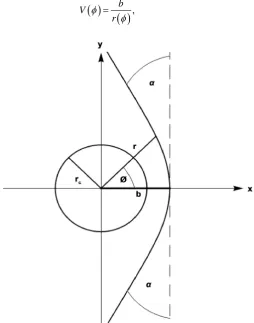
+ = (25)

[image:6.595.249.504.383.707.2]

Consider the trajectory of a photon outside the photon sphere showed in

Figure 1. The initial conditions are taken such that r_φ=0=b, and is called the impact parameter of the trajectory—the closest distance from the trajectory to the center of the black hole. We thus have,

0

d

0 d

r

φ

φ ₌ = and ₀

d

0 d

U

φ

φ ₌ = . The

photon experiences a total angular deflection of 2α. The smallest value of the r-coordinate in the trajectory, r=b, is taken such that the photon escapes the black hole, b>rc. We will rewrite Equation (25) in terms of 1

c

r b = <

 , which

we will use as a non-dimensional small number for our following perturbative expansions. Note that by multiplying both sides of Equation (25) by b, and defining the non-dimensional trajectory parameter

( ) ( )

b , V

r

φ

φ

= ₍₂₆₎

DOI: 10.4236/ijaa.2018.81009 127 International Journal of Astronomy and Astrophysics Equation (25), with the inclusion of the term rc

b =

 , then becomes a

differential equation in V

( )

φ : 2 2 2 d d V V V

φ

+ = (27)

where 0 rc 1

b

< = < , and with initial conditions given by

(

)

d

(

)

0 1; 0 0.

d

V

V φ φ

φ

= = = = (28)

Under these conditions, V

( )

φ is bounded such that

( )

1.

V φ ≤ (29)

5. First-Order Solution for

V

( )

φ

A first idea to obtain a solution of Equation (27) is to consider a V

( )

φ as a power series in :

( )

( )

( )

2

( )

0 1 2

;

V

φ

 =V

φ

+V

φ

+V

φ

+ (30) Plugging the expansion (30) into Equation (27) results in the following:

(

)

(

)

2 2 2

2 2

0 1 2

0 1 2

2 2 2

2 2

0 1 2

d d d

d d d

.

V V V

V V V

V V V

φ φ φ

  + + + + + + +     = + + +           (31)

We can group the powers of  in Equation (31): 2 0 0 0 2 d : 0 d V V

φ

+ =

 (32)

2

1 1 2

1 0 2 d : d V V V

φ

+ =

 (33)

2

2 2

2 0 1 2

d

: 2

d V

V V V

φ

+ =

 (34)

( )

2

2

3 3

3 1 0 2

2 d

: 2

d V

V V V V

φ

+ = +

 (35)



Note that the initial conditions of V

( )

φ , applied to the asymptotic expansion in Equation (30), imply the following, by grouping powers of :

( )

( )

0 0

0

d

: 0 1; 0 0

d

V V

φ

= =

 (36)

( )

d

( )

: 0 0; 0 0; 1.

d k k k V V k φ = = ≥

 (37)

From these differential equations and initial conditions, we can readily obtain

0

V and V1 iteratively (it is convenient to write the Vk

( )

φ in terms of

DOI: 10.4236/ijaa.2018.81009 128 International Journal of Astronomy and Astrophysics

( )

( )

0 cos

V φ = φ (38)

( )

( )

2

( )

1

2 1 1

cos cos .

3 3 3

V φ = − φ − φ (39)

Thus, we obtain an equation for V

( )

φ , per Equation (30):

( )

_cos

( )

2 1_cos

( )

1_cos2

( )

( )

2 _.

3 3 3

V φ = φ + _ − φ − φ _+O

 

  (40)

According to the coordinate system shown in Figure 1, the photon goes through a total angular deflection of 2α. This corresponds to setting V

( )

φ =0 for both φ=π 2+α _and φ= −π 2−α _{. From both of these conditions}

considering that α is very small, to first order in  we get: 2

3 _. 1

3

α

=

 ₋ 

 

 



 (41)

The total deviation of the photon is then

2

4

4 4

2 .

3 3

c

r GM

b bc

α

Ω = ≈ = = ₍₄₂₎

For a light ray grazing the Sun’s limb b=RΘ=695510 km [21] and we get the very well known value

2

4

2 GM 1.752 arcseconds

R c

α Θ

Θ

Ω = ≈ = ₍₄₃₎

where 30

1.9885 10 kg

MΘ= × is the Sun’s Mass, and

[ ]

6 2.99792458 10 m s

c= × is the value of the speed of light in vacuum [21].

6. Towards a Second-Order Solution for

Ω

( )

_

We will now see how to obtain higher-order solutions for Ω_{. The differential} equation in (34) has the following solution:

( )

( )

2

( )

3

( )

( )

2

4 41 2 1 5

cos cos cos sin .

9 36 9 12 12

V φ = − + φ + φ + φ + φ φ (44)

However, the term in Equation (44) that goes as φsin

( )

φ grows without bound, and occurs because the right-handed side of Equation (34) contains terms proportional to the homogeneous solution of Equation (34):

( )

( )

cos sin

a φ +b φ . When this happens, the solution contains terms that grow without bound, such as φsin

( )

φ , called secular terms [22]. Thus, if we naively include Equation (44) in V

( )

φ , our solution is no longer bounded. Thus, we have to eliminate any and all secular term that arises to arrive at a well-behaved solution for V

( )

φ .

One method to do this, due to Lindstedt and Poincaré, is by solving the differential equation in the following strained coordinate [22]:

(

2

)

1 2

1 .

DOI: 10.4236/ijaa.2018.81009 129 International Journal of Astronomy and Astrophysics where the ωk are constants to be determined. In terms of this new strained

coordinate φ_{, Equation (27) becomes}

(

)

2

( )

( )

2

2 2

1 2 2

d

1 .

d V

V V

ω

ω

φ

ε

φ

φ

+ +  +_{ } +  =  (46) We proceed in the previous way, and assume an asymptotic expansion on

( )

V φ :

( )

( )

( )

2

( )

0 1 2

;

V φ  =V φ +V φ +V φ + (47) Plugging the expansion(47) in Equation (46), we obtain:

(

)

(

) (

)

2 2 2

2

2 0 1 2 2

1 2 2 2 2

2

2 2

0 1 2 0 1 2

d d d

1

d d d

.

V V V

V V V V V V

ω ω

φ φ φ

  + + +  + + +    + + + + = + + +  _{  }             (48)

We can group the powers of  in Equation (48): 2 0 0 0 2 d : 0 d V V

φ

 + =

 (49)

2 2

1 1 2 0

1 0 1

2 2 d d : 2 d d V V

V V

ω

φ

 + = −

φ



 (50)

(

)

2

2 2

2 2 2 0 1

2 0 1 1 2 1

2 2 2

d

d d

: 2 2 2

d d d

V

V V

V V V

ω

ω

ω

φ

 + = − +

φ

 −

φ



 (51)

(

)

(

)

2 2

3 3 2 0

3 1 0 2 1 2 3

2 2

2 2

2 1 2

1 2 2 1 2

d d

: 2 2 2

d d

d d

2 2 .

d d

V V

V V V V

V V

ω ω ω

φ φ

ω ω ω

φ φ + = + − + − + −      (52)



With some care due to the definitions of the scaled variable and its derivative, we arrive at initial conditions for the Vk

( )

φ from the initial conditions of

( )

V φ :

(

)

( )

0 0

0

d

: 0 1; 0 0

d V V φ φ = = =  

 (53)

(

)

d

( )

: 0 0; 0 0; 1

d

k k

k

V

V φ k

φ

= = = ≥





 (54)

Solving the differential Equation (49) with initial conditions (53), we arrive at the zeroth-order contribution to V

( )

φ :

( )

( )

0 cos

V φ = φ (55) Similarly, we can obtain V1

( )

φ from Equation (50) subject to initial conditions (54):

( )

( )

2

( )

( )

1 1

2 1 1

cos cos sin .

3 3 3

DOI: 10.4236/ijaa.2018.81009 130 International Journal of Astronomy and Astrophysics freedom in the definition of ω1 to eliminate this secular term by setting

1 0

ω = (57) so that the final form of V1

( )

φ is:

( )

( )

2

( )

1

2 1 1

cos cos .

3 3 3

V φ = − φ − φ (58) Similarly we obtain for V2

( )

φ :

( )

( )

( )

( )

(

)

( )

2 2 3 2

4 5 2

cos cos

9 36 9

1 1

cos 144 60 sin .

12 144

V φ φ φ

φ ω φ φ

= − + +

+ + +

  

   (59)

To eliminate the secular term in V2

( )

φ , we set

2 5 12

ω

= − ₍₆₀₎

and obtain the well-behaved second-order term

( )

( )

2

( )

3

( )

2

4 5 2 1

cos cos cos .

9 36 9 12

V φ = − + φ + φ + φ (61)

From all the solutions obtained so far, we can obtain the second-order correction to Ω

( )

 . Note that V

( )

φ is given by:

( )

( )

( )

( )

( )

( )

( )

( )

2

2 2 3 3

2 1 1

cos cos cos

3 3 3

4 5 2 1

cos cos cos .

9 36 9 12

V

O

φ φ φ φ

φ φ φ

  = + _ − − _     + _− + + + _+             (62)

We set up φ=π 2+α in Equation (62), such that V

(

π 2+α

)

=0 and obtain:

( )

( )

( )

( )

( )

( )

( )

2

2 2 3 3

2 1 1

sin sin sin

3 3 3

4 5 2 1

sin sin sin 0.

9 36 9 12 O

α α α

α α α

  − + _ + − _     + _− − + − _+ =            (63)

We could truncate this Equation and solve the resultant cubic polynomial in

( )

sin α . However, this method would not be easy to generalize, because we do not have a general formula for the roots of fifth-order polynomials and above, according to Galois theory [23]. Also, an n-th order polynomial results in n different complex solutions, one of which we expect to have a leading term of order , to obtain a better approximation of Ω, and we would need to check all the n different solutions for this. Additionally, we have to remember that so far this is an asymptotic expansion in , and the truncation of the higher-order terms does not allow us to clearly see what the order of our estimate for Ω

( )



is. All of these problems are solved by assuming that sin

( )

α has the following expansion in , with a leading term of order 1

 :

( )

2 3

1 2 3

DOI: 10.4236/ijaa.2018.81009 131 International Journal of Astronomy and Astrophysics where the χk are constants to be determined. Inserting this new expansion into

Equation (63) leads to the following algebraic Equation:

( )

2 3 1 1 2 2 4 0.

3 9 3 O

χ

χ  χ 

 ₋  _{+ − + − + =}

   

     (65)

Then, we have to equal to zero the different powers of  in the last equation. Equating to zero the terms with _1 we arrive at:

1

2 3

χ = (66) and equating to zero the terms with _2 we arrive at:

2

2 . 9

χ = − ₍₆₇₎ Thus, sin

( )

α is given by:

( )

2 2 2

( )

3

sin .

3 9 O

α = −  +  (68) To obtain α, we employ the Taylor series of arcsin

( )

x around

x

=

0

:

( )

3

( )

5

arcsin

6

x

x = +x +O x (69)

and obtain

( )

2 3

2 2

.

3 9 O

α= −  +  (70) However, what we actually want is α. From the definition of the strained coordinate φ in (45), it is clear that:

( )

2 3 1 2 π π ₂ .

2 1 O

α α ω ω + + = + + + 

   (71)

From the last equation, an using the Taylor expansion of

( )

0 1 1 1 n n n x x ∞ = = −

+

∑

around

x

=

0

, we obtain:

( )

2 3

2 5π 2

3 24 9 O

α= +_ − _ +

 

   (72)

From which we can obtain the total deflection angle,

Ω =

2α

( )

2 3

2 3

2 2 2

4 5π 4

3 12 9

4 15π

4 .

4

O

GM GM GM

O

bc bc bc

 

Ω = +_ − _ +

         = +_ − _{ } + _{ }     _  _    (73)

This result is in agreement with other work [12][13][14][15].

7. Higher Order Solutions for

Ω

( )

_

DOI: 10.4236/ijaa.2018.81009 132 International Journal of Astronomy and Astrophysics Ω_{. Notably, all the solutions for the} V_k

( )

φ are in the forms of

(

k+1

)

-order polynomials of cos

( )

φ , and a secular term that is eliminated by choosing a

suitable ωk. The use of the expansion of sin

( )

α in powers of  guarantees

both the form of sin

( )

α with a leading term of order , and leads to algebraic equations for the χk that are exceedingly easy to solve. Notably,

getting a higher-order solution conserves the lower-order terms. Consider the formal Taylor expansion of Ω _around



=

0

:

1 2 3

1 2 3

κ κ κ

Ω =  +  +  +_ (74) A table of the coefficients κn of the series of Ω in (74) can be found in

Table 1. These κn were found using the method of the previous sections, and

obtaining the solutions up to V20

( )

φ .

Clearly, as



→

1

, Ω

( )

 → ∞, because the photon starts going around the

black hole as it starts closing in the photon sphere (b→rc). This means that

( )

Ω  has a singularity at =1. The Taylor expansion of Ω

( )

 around



=

0

that we found at Equation (74) does not return an estimate for the position of this singularity, because a polynomial does not have a singularity. However, we can obtain Padé approximants for Ω _around



=

0

, and these will return an

estimate for the position of this singularity.

As a small refresher on Padé approximants, we note their definition. A Padé approximant of a function f x

( )

is a rational function f[L M| ]

( )

x of the form:

[| ]

_{( )}

0 1 2 2

2

1 2

1

L

L M L

M M

a a x a x a x

f x

b x b x b x

+ + + +

=

+ + + +



 (75)

where f x

( )

and [ | ] ( )

L M

f x are equal in their first L+M+1 derivatives

around

x

=

0

[24] [25]. A diagonal Padé approximant [ ]N

( )

f x is a Padé approximant in which

N

= =

L

M

. We can obtain the diagonal Padé approximants for up to N = 10 with the Taylor series expansion for Ω

( )

 . For example, the _Ω[ ]1

( )

 Padé approximant is given by:

[ ]

_{( )}

(

)

(

)

2 1 48π 64 16π 15π

. 96 32 30π

+ + −

Ω =

+ −

 

 (76)

The exact formulas for the Padé approximants of Ω

( )

 are rather complicated because of the powers of π involved. Due to this, our work with Padé approximants will be purely numeric. All the Padé approximants _Ω[ ]N

( )

 have a singularity of order 1 at a position around =1. The position of this

singularity, s, is tabulated for the 10 Padé approximants in Table 2.

8. Numerical Tests for

Ω

(

λ

) and Its Padé Approximants

All the coefficients for the Taylor expansion of Ω

( )

 were obtained around

0

=



. We can test the correctness of the methods thus far used to obtain this function by comparing it to the results of numerical solutions of Equation (22). This is done with both truncated n-th order Taylor polynomials from Ω

( )



[image:13.595.207.540.104.631.2]

DOI: 10.4236/ijaa.2018.81009 133 International Journal of Astronomy and Astrophysics

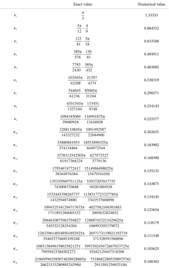
Table 1. Coefficients κn of the series of Ω in (74). For these coefficients, we report both the exact values and the numerical values with 6 significant figures.

Exact value Numerical value

1

κ 4

3 1.33333 2

κ 5π 4

12−9 0.864552 3

κ 122 5π

81−18 0.633508 4

κ 385π 130

576 − 81 0.494911 5

κ 7783 385π

2430− 432 0.403082 6

κ 103565π 21397

62208 − 4374 0.338319

7

κ 544045 85085π

61236 −31104 0.290571

8

κ 6551545π 133451

1327104 − 8748 0.254143

9

κ 1094345069 116991875π

39680928 − 13436928 0.225577

10

κ 2268110845π 1091492587

143327232 − 22044960 0.202655

11

κ 33880841953 18553890355π

374134464 − 644972544 0.183902

12

κ 3278312542505π 627972527

61917364224 − 3779136 0.168300

13

κ 17954674772417 1514986498025π

58364976384 − 15479341056 0.155132

14

κ 135335969751125π 53937207017735

743008370688 − 94281884928 0.143875

15

κ 1532445398265737 1138317723327785π

1432594874880 − 3343537668096 0.134145

16

κ 1094325341294717675π 4027582104301883

1711891286065152 − 2005632824832 0.125654

17

κ 2064610875963794827 128887453213429625π

545532128354304 − 106993205379072 0.118179

18

κ 1263396148548501892925π 2657173119021192719

554652776685109248 − 371328591568896 0.111548 19

κ 1085138496158025821251 399330245672667033725π

79959423384502272 − 92442129447518208 0.105625 20

κ 218695963585074038928865π 75186822805298075761

26623333280885243904 − 2913501256925184 0.100303

[image:14.595.207.538.92.508.2]

DOI: 10.4236/ijaa.2018.81009 134 International Journal of Astronomy and Astrophysics

Table 2. The position of the singularity near =1 for the Padé approximants, Ω[ ]N

( )

 .

N s

1 1.54222

2 1.21736

3 1.11036

4 1.06664

5 1.04532

6 1.03238

7 1.0245

8 1.01915

9 1.01537

10 1.01264

Figure 2. Numerical points obtained for Ω

( )

 compared to the truncated n-th order Taylor polynomials of Ω

( )

 , up to 20-th order. With increasing value of n, the polynomials take larger values.

that have singularities [25]. Once we know that the Ω

( )

 behave correctly, we can use the Ω

( )

 to simulate the bending of light around a black hole. A simple first-order ray tracing algorithm that does this for the different approximations of Ω

( )

 we have found is shown in the next section.

9. Ray tracing Using

Ω

( )



[image:15.595.210.535.64.288.2]

DOI: 10.4236/ijaa.2018.81009 135 International Journal of Astronomy and Astrophysics

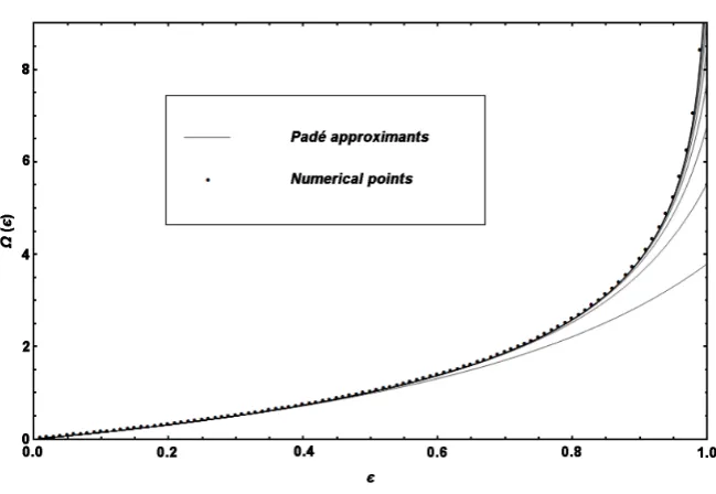
Figure 3. Numerical points obtained for Ω

( )

 compared to the truncated N-th diagonal Padé approximants of Ω

( )

 , up to N=10. With increasing value of N, the

Padé approximants take larger values. For =0.99, the N=10 Padé approximant is

within 3% of the numerical value of Ω

( )

 .

( )

,

A

I θ φ , in spherical coordinates. Now, imagine another point in space, B, far enough from the observer A such that the intensity of light that comes from every point in the sky, according to an observer in point B, is also given by the distribution found by observer A: IB

( )

θ φ, =IA

( )

θ φ, . If we place a black hole at point B, then light coming from the faraway sources will bend around the black hole such that the original observer will see a different distribution of light around the black hole. In this condition, the observer will be able to note that the black hole effectively subtends a solid angle in the sky—region in the sky devoid of any light due to the black hole. One half of the angle subtended by the black hole will effectively give the “angular radius” of the black hole, as seen by the observer, rBH.

If we consider that the black region of the sky due to the black hole is due to the radius of the photon sphere, rc, instead of the the Schwarzschild radius, rs,

and if we choose the coordinate system such that the black hole is at the positive x-axis, θ =π 2 _and φ=0, then, by definition of r_BH, the new distribution of light measured by the observer will obey (for small enough rBH):

(

)

(

)

2 2

( )

2

, 0; π 2 _BH .

I θ φ = θ− +φ ≤ r (77) For other values of

( )

θ φ, , the observer sees light distribution shifted by the

( )

Ω _{ , where  is given for} θ ≈π 2 by:

(

)

2 2

. π 2

c BH

r r

b _{θ φ}

= =

− +

 (78)

DOI: 10.4236/ijaa.2018.81009 136 International Journal of Astronomy and Astrophysics that grazes the black hole at a distance given by r=b. This trajectory of this light is bended by the black hole for b>rc. However, if b<rc, the light will not

escape and effectively no light coming from faraway objects will seem to originate from r<rc, which becomes an effective radius for the black hole,

according to observer A in these conditions. In the case that mass enters the black hole, and emits light from an r that obeys rs< <r rc, the light can escape

the black hole, and is severely red-shifted. However, we are here considering a black hole with no light sources between rs < <r rc.

We can use a further simplification of Equation (78), and use the coordinates

(

θ θx, y

)

defined by θx=φ,

θ

y = −

θ

π 2. For small values of θx and

θ

y, say,

in the order of milliradians, we can write:

(

)

2 2

( )

2

, 0;

x y x y BH

I

θ θ

=

θ

+

θ

≤ r (79) and

2 2

BH

x y

r

θ

θ

= +

 (80)

where the analogue with Cartesian coordinates is evident. This coordinate system is shown in Figure 4 for a black hole that subtends _{4π 10×} −6 _steradians, such that rBH =2 mrad.

This coordinate choice allows one to define the distribution of intensities that observer A sees to be (disregarding some attenuation factors):

(

)

( )

( )

2 2 2 2

, x , y ;

x y A x y

x y x y

I θ θ I θ θ θ θ

θ θ θ θ

 

 

= − Ω − Ω

 _{+ +} 

 

  (81)

where 2 2

( )

2

x y rBH

θ +θ ≤ and we have used I_A

(

θ θ_x, _y

)

, the angular distribution

of intensities seen by observer A without the black hole present, and using the coordinates

(

θ θ_x, _y

)

. We can see the effect of applying Equation (81) by using

the I_A

(

θ θ_x, _y

)

defined from Figure 5.

To model the deflection of light with the distribution in Figure 5, we use Equation (81) with Ω

( )

 approximated as a truncated first-degree Taylor polynomial, and as diagonal Padé approximants with N =2 and N=10. The resulting images can be found in Figures 6-8. We use a black hole with

10

BH

r = mrads.

The most notable difference between Figure 6 and Figure 7 is the position of the white ring around the black hole, corresponding to the gravitational lensing of the big, white star at the black hole position

θ

_y=0. When using a better approximation of Ω

( )

 , this ring has greater inner and outer radii, and is thinner. In Figure 8, there are 8 white pixels around 2 2

10

x y

θ

+

θ

= millirads, corresponding to a second ring of light due to the big, white star.

10. Conclusions and Suggestions

[image:17.595.209.538.70.369.2] [image:17.595.269.475.416.614.2]

DOI: 10.4236/ijaa.2018.81009 137 International Journal of Astronomy and Astrophysics

Figure 4. A black hole with rBH=2 mrad in the center of the

(

θ θx, y

)

coordinate

system.

Figure 5. 600 600× image corresponding to the

intensity due to background light sources, I_A

(

θ θ_x, _y

)

,

without a black hole present. Each pixel corresponds to 1 mrad. The big star, in white, has a radius of 50 mrad. The small stars, in gray, have a radius of 3 mrad. The star is at the center of the coordinate system,

[image:18.595.251.495.70.324.2]

DOI: 10.4236/ijaa.2018.81009 138 International Journal of Astronomy and Astrophysics

Figure 6. Background of Figure 5 warped by a black hole at (a)

300

y

θ = mrad, (b) θ_y=200 mrad, (c) θ_y =100 mrad, and

(d) θy=0 mrad. We make use of the truncated first-order Taylor

polynomial of Ω

( )

 .

Figure 7. Background of Figure 5 warped by a black hole at (a)

300

y

θ = mrad, (b) θ_y =200 mrad, (c) θ_y =100 mrad, and (d) 0

y

[image:18.595.249.500.406.662.2]

[image:19.595.248.499.76.349.2]

DOI: 10.4236/ijaa.2018.81009 139 International Journal of Astronomy and Astrophysics approximant of Ω

( )

 .

Figure 8. Background of Figure 5 warped by a black hole at (a)

300

y

θ = mrad, (b) θ_y =200 mrad, (c) θ_y =100 mrad, and (d) 0

y

θ = mrad. We make use of the diagonal N=10 Padé

approximant of Ω

( )

 .

or even a galaxy (in this case it can generate a gravitational lens). In this paper using the Schwarzschild metric we have obtained higher order corrections for the gravitational deflection of light around said objects using the Lindstedt- Poincaré method to solve the equation of motion of a photon around the stellar body. We have successfully obtained an expression for Ω

( )

 , the angular deflection experienced by a photon traveling around the massive object. We have assumed that the parameter  was small, and we were able to obtain the coefficients κn of the series of Ω

( )

 up to V20

( )

φ (the non-dimensional trajectory parameter, see equation (26)). The results are given in Table 1. Additionally, we have obtained diagonal Padé approximants from the perturbation expansion, and we have shown how these are a better fit for the numerical data. The best approximation for Ω

( )

_{ we obtained was consistent with the}

numerical data even for an ≈0.99. In this case, the N =10 diagonal Padé approximant is within 3% of the corresponding numerical value. We were able to use this estimate for Ω

( )

 in ray-tracing algorithms to model the bending of light around the massive object.

Acknowledgements

DOI: 10.4236/ijaa.2018.81009 140 International Journal of Astronomy and Astrophysics was funded by the Universidad San Francisco de Quito USFQ Research Publica-tion Fund.

References

[1] Einstein, A. (1915) Die feldgleichungen der gravitation, Sitzungsberichte der König-lich Preussischen Akademie der Wissenschaften zu Berlin.

[2] Einstein, A. (1916) Die grundlage der allgemeinen relativitätstheorie. Annalen der Physik, 354, 769-822.https://doi.org/10.1002/andp.19163540702

[3] Ohanian, H.C. (1976) Gravitation and Spacetime. W. W. Norton & Company, Inc., New York.

[4] Weinberg, S. (1972) Gravitation and Cosmology. Wiley & Sons, Inc., New York. [5] Weinberg, S. (1989) The Cosmological Constant Problem. Reviews of Modern

Physics, 61, 1-23. https://doi.org/10.1103/RevModPhys.61.1

[6] Weinberg, S. (2008) Cosmology. Oxford University Press, Oxford, 43-44.

[7] Hobson, M.P., Efstathiou, G. and Lasenby, A.N. (2006) General Relativity. An In-troduction for Physicists. Cambridge University Press, Cambridge.

https://doi.org/10.1017/CBO9780511790904

[8] Wald, R.M. (1984) General Relativity. University of Chicago Press, London, 453-456. https://doi.org/10.7208/chicago/9780226870373.001.0001

[9] Carroll, S.M. (2004) An Introduction to General Relativity. Addison Wesley, Bos-ton, 162-172.

[10] Hawking, S.W. (1988) A Brief History of Time. From the Big Bang to Black Holes. Bantam Dell Publishing Group, New York.

[11] Lebach, D.E., et al. (1995) Measurement of the Solar Gravitational Deflection of Ra-dio Waves using Very-Long-Baseline Interferometry. Physical Review Letters, 75, 1439-1442.https://doi.org/10.1103/PhysRevLett.75.1439

[12] Bodenner, J. and Will, C. (2003) Deflection of Light to Second Order: A Tool for Il-lustrating Principles of General Relativity. American Journal of Physics, 71, 770-773.https://doi.org/10.1119/1.1570416

[13] Fischback, E. and Freeman, B.S. (1980) Second Order Contribution to the Gravita-tional Deflection of Light. Physical Review D, 22, 2950-2952.

https://doi.org/10.1103/PhysRevD.22.2950

[14] Richter, G.W. and Matzner, R.A. (1982) Second Order Contributions to Gravita-tional Deflection of Light in the Parametrized Post-Newtonian Formalism. Physical Review D, 26, 1219-1224. https://doi.org/10.1103/PhysRevD.26.1219

[15] Epstein, R. and Shapiro, I. (1980) Post-Post-Newtonian Deflection of Light by the Sun. Physical Review D, 22, 1219-1224. https://doi.org/10.1103/PhysRevD.22.2947

[16] Shchigolev, V. and Bezbatko, D. (2016) Studying Gravitational Deflection of Light by Kiselev Black Hole via Homotopy Perturbation Method.

[17] Claudel, C., Virbhadra, K.S. and Ellis, G.F.R. (2001) The Geometry of Photon Sur-faces. Journal of Mathematical Physics, 42, 818-838.

https://doi.org/10.1063/1.1308507

[18] Misner, C., Thorne, K. and Wheeler, J. (1973) Gravitation. W. H. Freeman & Com-pany, New York, 607.

DOI: 10.4236/ijaa.2018.81009 141 International Journal of Astronomy and Astrophysics 128-130. https://doi.org/10.1007/978-1-4020-4523-3

[21] Olive, K.A. (2014) Particle Physics Booklet. Particle Data Group, Chin. Phys. C., 38, No. 9.

[22] Bush, A. (1992) Perturbation Methods for Engineers and Scientists. CRC Press, Bo-ca Raton.

[23] Tignol, J. (2002) Galoi’s Theory of Algebraic Equations. World Scientific, Singa-pore.

[24] Saff, E. and Varga, R. (1977) Padé and Rational Approximation. Academic Press, Cambridge.