warwick.ac.uk/lib-publications
Manuscript version: Author’s Accepted Manuscript
The version presented in WRAP is the author’s accepted manuscript and may differ from the
published version or Version of Record.
Persistent WRAP URL:
http://wrap.warwick.ac.uk/126413
How to cite:
Please refer to published version for the most recent bibliographic citation information.
If a published version is known of, the repository item page linked to above, will contain
details on accessing it.
Copyright and reuse:
The Warwick Research Archive Portal (WRAP) makes this work by researchers of the
University of Warwick available open access under the following conditions.
Copyright © and all moral rights to the version of the paper presented here belong to the
individual author(s) and/or other copyright owners. To the extent reasonable and
practicable the material made available in WRAP has been checked for eligibility before
being made available.
Copies of full items can be used for personal research or study, educational, or not-for-profit
purposes without prior permission or charge. Provided that the authors, title and full
bibliographic details are credited, a hyperlink and/or URL is given for the original metadata
page and the content is not changed in any way.
Publisher’s statement:
Please refer to the repository item page, publisher’s statement section, for further
information.
Polylogarithmic Guarantees for
Generalized Reordering Buffer Management
Matthias Englert
DIMAP and Department of Computer Science University of Warwick
Coventry, UK [email protected]
Harald R¨acke Department of Informatics Technical University of Munich
Munich, Germany [email protected]
Richard Stotz Department of Informatics Technical University of Munich
Munich, Germany [email protected]
Abstract— In the Generalized Reordering Buffer Manage-ment Problem (GRBM) a sequence of items located in a metric space arrives online, and has to be processed by a set of k
servers moving within the space. In a single step the first b
still unprocessed items from the sequence are accessible, and a scheduling strategy has to select an item and a server. Then the chosen item is processed by moving the chosen server to its location. The goal is to process all items while minimizing the total distance travelled by the servers.
This problem was introduced in [Chan, Megow, Sitters, van Stee TCS 12] and has been subsequently studied in an online setting by [Azar, Englert, Gamzu, Kidron STACS 14]. The problem is a natural generalization of two very well-studied problems: thek-server problem forb= 1and the Reordering Buffer Management Problem (RBM) fork= 1. In this paper we consider the GRBM problem on a uniform metric in the online version. We show how to obtain a competitive ratio of O(logk(logk+ log logb)) for this problem. Our result is a drastic improvement in the dependency on b compared to the previous best bound ofO(√blogk), and is asymptotically optimal for constantk, becauseΩ(logk+log logb)is a lower bound for GRBM on uniform metrics.
I. INTRODUCTION
In the Generalized Reordering Buffer Management Prob-lem (GRBM) a sequence of items located in a metric space arrive online, and have to be processed by a set ofkservers moving within the space. In a single step the first b still unprocessed items from the sequence are accessible, and a scheduling strategy has to select an item and a server. Then the chosen item is processed by moving the chosen server to its location. The goal is to process all items while minimizing the total distance travelled by the servers.
This problem was introduced by Chan et al. [18] and has subsequently been studied in an online setting by Azar et al. [10]. It is a natural generalization of two very well-studied problems: thek-server problem forb= 1[32] and the Reordering Buffer Management Problem (RBM) fork= 1 [33]. RBM and GRBM can be used for modeling context switching cost that occur in applications in many different areas ranging from production engineering through computer graphics to information retrieval (see e.g. [8], [10], [14], [30]). In this paper we consider the GRBM problem on a
uniform metric in the online version in which the scheduling strategy does not know future items in the input stream but has to make its decisions only depending on the sequence of items it has seen so far.
Since the RBM problem is just the GRBM problem with
k= 1a lower bound ofΩ(log logb)on the competitive ratio of RBM in uniform metrics (see [2]) applies also to GRBM. Another lower bound ofΩ(logk)stems from the fact that for
b= 1 the GRBM problem is just the well knownk-server problem which, for uniform metrics (the paging problem), has a well-known lower bound ofΩ(logk)[23].
The best upper bound on the competitive ratio for uniform metrics is due to Azar et al. [10] who gave a guarantee of O(√blogk). In this paper we drastically reduce the dependency onbin the upper bound and present an algorithm that obtains a competitive ratio ofO(logk(logk+ log logb)).
One potential approach for obtaining an algorithm for GRBM would be to extend an algorithm for RBM (e.g. the optimal algorithm for RBM by Avigdor-Elgrabli and Rabani [8]) to several servers. However, due to the complexity of this algorithm this approach seems challenging. Hence, we proceed differently. A major building block of our algorithm is a buffer management strategy for block-devices as introduced in [3]. The block device model is closely related to RBM on a uniform metric and can be described as follows. The metric space is formed by a (uniform) star and the items appear at the leaf vertices of this star, while the server is located at the center. In a single step the server may visit a leaf vertex v, process all items located at v, and then return to the center. Such a step is called a block operation (on vertexv) and induces a cost of1. The difference between both models is that in RBM the server could stay at
v and also process subsequent items that appear there. This seemingly subtle difference between the models means that the optimum cost for serving a request sequence may differ widely between the block-device model and RBM. An input consisting of a sequence of` requests for a single vertex for example could be served with cost 1 in the RBM model, but would result in cost of `/bin the block-device model.
-competitive algorithm for scheduling block-devices. In con-trast to the RBM problem, the block-device version of the problem can be easily formulated as a covering linear program, which allows a fairly straightforward application of the standard online primal-dual framework by Buchbinder and Naor [17].
The rough idea behind our approach is to allow the algorithm to perform block operations in addition to using thekservers. Note that in a uniform metric, we can simulate a block operation with constant cost (pick any of the k
servers, move it to the desired vertex to process all items there, and immediately move it back to its original position) and therefore this addition does not really change the model. We then perform block operations according to the algorithm given in [3].
This actually means that we only apply the online primal-dual scheme to a part of the LP (some of the variables and some of the constraints). We then complement this with a second procedure which handles the remaining parts. This procedure solves the sub-problem of placing thek servers and will be a variant of the paging problem.
In other words, we solve our problem by splitting it into the part that is amenable to be dealt with by an online primal-dual scheme and the remaining part which is then tackled by other means. This way we are able to solve a problem which otherwise seems out of reach for the online primal-dual framework.
This split into two parts turns out to be useful for another reason as well. For one part we can utilize prior insights from paging and for the other part we can rely on prior insights from block-device scheduling. However, note that in particular the paging related sub-problem is still significantly more challenging than a standard paging problem (see e.g. [23], [34]) and requires new techniques. We briefly discuss this as part of Section III-B1.
Finally, we note that, as a special case (with k = 1), we obtain a newoptimalalgorithm for RBM which is very different from the one by Avigdor-Elgrabli and Rabani [8] further contributing to our understanding of this well-studied problem. Indeed, if we were only interested to obtain this result fork= 1, our algorithm and proof could be simplified significantly. For example, Section V is not needed at all for this case.
Further Related Work
There is a vast literature on the k-server and RBM problems, see for example [1], [12], [16], [29], [31] and [4], [13], [19], [20], [22], [24], [25], [26], [27], [28] respectively. We limit our discussion to the results most closely related to ours. The RBM problem for uniform metrics was introduced by R¨acke et al. [33] who gave a deterministic algorithm with competitive ratio O(log2b). This was subsequently improved by Englert and Westermann [21] to O(logb), by Avigdor-Elgrabli and Rabani [9] toO(logb/log logb)and by
Adamaszek et al. [2] toO(√logb). The latter result is close to optimal due to a lower bound ofΩ(plogb/log logb)for deterministic algorithms shown in the same paper.
For the randomized case Avigdor-Elgrabli and Rabani [8] developed an online algorithm with optimum competitive ratioO(log logb). Avigdor-Elgrabli et al. [6] extended this to the case of a star-metric space, i.e., where the points in the metric space are leaves of a star with arbitrary edge-length. For this scenario they obtain a competitive ratio of O((log log(b∆))2), where∆ is the ratio between the length
of the longest and shortest edge.
For the offline variant Asahiro et al. [5] and Chan et al. [18] independently established the NP-hardness of the problem on uniform metrics. Avigdor-Elgrabli and Rabani [7] designed a constant factor approximation algorithm for this offline setting.
A related problem is the Online Service with Delay problem (OSD-problem) introduced by Azar et al. [11]. In this problem items appear in a metric space but there is no upper bound on the number of unprocessed items at any given time (like the buffer-sizebin GRBM). Instead the items come with delay penalty functions that ensure that eventually items have to be processed as otherwise the accumulated delay penalty would become too large. The goal is to minimize the total distance traveled by the servers plus the total delay penalty. For infinite delay penalties this problem reduces to paging (for a uniform metric) and to k-server (general metric), respectively.
Azar et al. give a competitive ratio of O(kpolylogn)
for arbitrary metrics and show that for uniform metrics the problem is the paging problem, which gives a competitive ratio ofO(logk).
II. MODEL
In this section we give the precise definition of our model. As is common in the RBM problem we refer to the individual locations within the uniform metric space as colors. For notational convenience we assume that at any point in time the buffer can storeb+ 1items (the difference between b
andb+ 1does not affect our asymptotic results). At the start of a step, a new item appears and is brought into the buffer. If this item has a color that currently has a server assigned to it we directly remove the item again and proceed to the next step. Otherwise, it might happen that now the buffer containsb+ 1items. Then we cannot proceed to the next time step but we first have to remove at least one item from the buffer. We can do this by selecting a colorcand either perform a block operation for c or re-assign one of the k
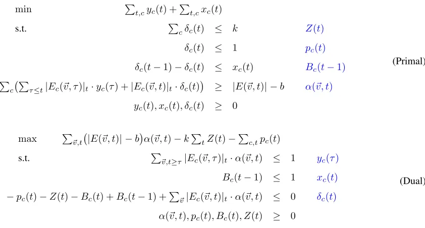
servers toc. In both cases all items of colorc are removed from the buffer. The goal is to minimize the total number of operations. Our LP formulation is Primal as shown in Figure 1 withδc(0) = 0 for all colorsc.
We introduce variables δc(t), andyc(t)for every color c
min P
t,cyc(t) +Pt,cxc(t)
s.t. P
cδc(t) ≤ k Z(t)
δc(t) ≤ 1 pc(t)
δc(t−1)−δc(t) ≤ xc(t) Bc(t−1)
P
c
P
τ≤t|Ec(~v, τ)|t·yc(τ) +|Ec(~v, t)|t·δc(t)
≥ |E(~v, t)| −b α(~v, t)
yc(t), xc(t), δc(t) ≥ 0
(Primal)
max P
~v,t |E(~v, t)| −b
α(~v, t)−kP
tZ(t)−
P
c,tpc(t)
s.t. P
~v,t≥τ|Ec(~v, τ)|t·α(~v, t) ≤ 1 yc(τ)
Bc(t−1) ≤ 1 xc(t)
−pc(t)−Z(t)−Bc(t) +Bc(t−1) +P
~v|Ec(~v, t)|t·α(~v, t) ≤ 0 δc(t) α(~v, t), pc(t), Bc(t), Z(t) ≥ 0
[image:4.612.136.557.75.301.2](Dual)
Figure 1. Primal and dual linear program used by our algorithm.
is a server at color c at the end of step t and yc(t) = 1
means that we perform a block operation forc in stept. The
Z(t)-constraints ensures that we use at most kservers while thepc(t)-constraint ensures that we do not move more than one server to any location. If we want to move a server away from a colorc, i.e., if δc(t−1)−δc(t) = 1, theBc(t−1) -constraint ensures that we have to pay for this move by settingxc(t) = 1. Note that in our uniform model we do not pay the distance that a server travels, but we simply pay 1 for every server move.
It remains to model the buffer constraint. For this we introduce the following notation. For two vectors~u, ~vof time steps (one entry for every color) we useEc(~u, ~v) to denote the items of colorcthat arrived in time-interval(uc, vc] (we also allowuc= 0in the vector so that also the first item can be in such a set). We define E(~u, ~v) :=S
cEc(~u, ~v). We
extend this notation to the case where the second parameter is a scalar with the meaning that all entries of the corresponding vector are equal to this scalar: Ec(~u, t) :=Ec(~u, ~v) with
vc=t for allc(similarly forE(~u, t)).
LP Primal is not a faithful representation of the problem as an integral solution does not necessarily satisfy all constraints. However, we can modify any solution in such a way that the cost increases by a factor of at most 2 and the modified solution does satisfy the LP. Specifically, take any solution and whenever one of thekservers is moved away from color
c (i.e.δc(t−1) = 1 and δc(t) = 0), we perform a block operation for colorc(i.e.,yc(t) = 1). Note that this increases the cost by a factor of at most 2. Concretely, it may increase P
t,cyc(t)in the objective function, but it increases it by at
mostP
t,cxc(t).
A solution modified in this way, now satisfies α(~v, t)
constraints. Consider the items in a setE(~v, t). How many of these items are we removing by timet? Clearly, a block operation for colorc at timeτ removes at most |Ec(~v, τ)| of these items. A server that leaves at timeτ < talso can remove at most|Ec(~v, τ)| of these items. However, since a leave event is co-located with a block operation we actually do not need to count the items that are removed by servers that left before timet as these are counted via the corresponding block operation. In case a server is located atcat timetthis server can remove at most|Ec(~v, t)| items. Hence,
X
c
X
τ≤t
|Ec(~v, τ)| ·yc(τ) +|Ec(~v, t)| ·δc(t)
≥ |E(~v, t)| −b
is a valid constraint as the left hand side is an upper bound on the number of items that we removed and the right hand side is a lower bound on the number of items from
E(~v, t)that we need to remove in order to fulfill the buffer constraint at timet. Theα(~v, t)constraint in the primal linear program is a strengthening of this constraint where we define |Ec(~v, τ)|t := max{0,min{|Ec(~v, τ)|,|E(~v, t)| −b}}. For
dual problem is Dual shown in Figure 1.
A. Modifying the Linear Program
A crucial ingredient for the analysis of the block-device scenario [3] and the RBM setting [8] is that a slight change in the buffer size only changes the competitive ratio by a constant factor. An analogous property holds for the GRBM problem and is proven in the appendix.
Theorem 1. For any input sequence, the costOPTb0 of an
optimal offline solution utilizing a buffer of sizeb0= (1−ε)·b
is at most a factor of (2 +εlnb0)/(1−ε)larger than the costOPTb of an optimal offline solution utilizing a buffer
of size b.
This theorem allows us to change b into b0 = (1 −
1/logb)·b, in LP Primal while only increasing the op-timum solution value by a constant factor. In the new LP the capping is done w.r.t. b0, i.e., |Ec(~v, τ)|t :=
max{0,min{|Ec(~v, τ)|,|E(~v, t)| −b0}}.
We then remove allα(~v, t)-constraints for pairs(~v, t)with |E(~v, t)| ≤b, which cannot increase the optimum solution value. This means that now we have|E(~v, t)| −b0≥b/logb
for everyα(~v, t)-constraint.
Corollary 2. The value of the modified LP is at most a constant factor larger than the cost OPTb of an optimal
offline algorithm using a buffer of size b.
B. Introducing Dummy Steps
Purely to simplify the presentation of our algorithm and our proofs we introduce dummy time steps. These are time steps in which no new item arrives. We assume that between any two real time steps (in which an item arrives) there are an arbitrarily large number of dummy time steps. In fact, for ease of presentation, we allow the algorithm to make infinitesimal changes to variables during a time step. Alternatively, this can be thought of as sufficiently small discrete steps.
Our algorithm has to ensure that at the start of each real time step, there are at most b items stored in the buffer, so that the new item arriving in the real time step can be accommodated.
III. THEALGORITHM
Our algorithm consists of two main parts. The first part is thebase procedureand only performs block operations. The base procedure can run on its own and produce a feasible solution to the problem. However, because it does not utilize thek servers and exclusively performs block operations, the cost of such a solution may be too large.
The second part of our algorithm is thecost control proce-dure. This procedure schedules additional block operations and, crucially, determines the placement of thek servers in such a way that the base procedure can produce a feasible
solution with fewer block operations. The goal is to do this in such a way that, overall, our cost is greatly reduced.
The base procedure will (fractionally) increasey-variables in the primal in conjunction with producing assignments for the dual α-variables. It also has a randomized rounding procedure for the y-variables which produces the final schedule of block operations that ensure the buffer constraint (i.e. ensure that at the start of each real time stept no more thanb items are stored in the buffer).
The cost control procedure integrally sets primal y -variables to 1 at certain points in time (in other words, performs a block operation) and assigns integer values to theδ- andx-variables (in other words, places thek servers). While the cost control procedure only sets variables in the LP integrally, and therefore does not require a rounding routine, the procedure itself is randomized and vaguely inspired by the well known randomized marking algorithm for paging.
The base procedure largely follows [3]. The only material difference is that we have to take theδ-variables of the LP into account. In [3], the last time step at which a block operation to a color occurred, played a special role because we know that all items of that color arriving before that operation are not stored in the buffer anymore. Now, we need to change this to say “last time step at which either a block operation to colorcoccurred, or a server was located atc”.1 This is reflected in the inclusion ofδ-variables in the definition of aproper constraintin the following section.
Our main contribution is the cost control procedure as well as the insight that the problem can be nicely separated into these two parts which, arguably, simplifies the algorithm design and analysis.
A. The Base Procedure
We now start by discussing the base procedure. Before we describe the procedure in more detail, we introduce the notion of aproperconstraint. This uses a constant scaling factorβ := 40.
Definition 3. For a given variable assignment, an α(~z, t)
constraint in the primal is called proper if the following holds for every colorc:
(i) P
zc≤τ≤t(yc(τ) +δc(τ))≥1/β, (ii) P
zc<τ≤t(yc(τ) +δc(τ))<2/β, and
(iii) yc(τ) +δc(τ)<1/β for all τ∈ {zc+ 1, . . . , t}.
Note that in particular, because of (iii), if δc(τ) = 1 or
yc(τ) = 1, then for a proper constraintα(~z, t)we must have
zc ≥τ.
The base procedure maintains a vector ~z such that the primalα(~z, t)constraint is proper for the current time step
t. If the current α(~z, t)constraint is violated, the procedure increasesy-variables of the primal using the standard online
1This is only an intuition, because we actually have to deal with fractional
primal-dual approach by Buchbinder and Naor [17]. This continues until the constraint is not proper anymore (in which case~zis updated) or until the constraint is satisfied (in which case the procedure progresses to the next real time step and receives the next item from the input). More precisely, if at any time,α(~z, t)is not proper (due to previous increases of
δ- ory-variables), we recompute~z by setting, for each color
cfor which one of the conditions is violated,zcto the largest possible value (less or equal tot) such thatP
zc≤τ≤t(yc(τ)+
δc(τ))≥1/β. While not exactly true, intuitively,zc can be thought of as (roughly) the largest time such that every item of colorcwhich arrived before that time has been completely removed from the buffer.
The base procedure also maintains a second vector~s. The default is thatsc =zc for every colorc. However, at certain points, the cost control procedure in our algorithm can decide to setsc< zc for some specific color and then “freeze” that value ofsc. That means that later updates ofzc are ignored forscandscremains fixed until we “unfreeze” it. To describe this state or event we say that color cis or becomes active. Once we unfreeze a color,sc is set to be equal to zc again.
We then say that the color isdeactivated. When we decide to make a color active, the precise value of sc is chosen
such that|Ec(~s, ~z)|=dfmaxe, withfmax:= (b−b0)/2k= b/(2klogb). The precise way in which colors are activated and deactivated is described later.
After the base procedure updates values of the (fractional)
y-variables, it uses an (online) randomized rounding proce-dure to determine which block operations to execute. For this, the procedure updates a probabilistic distributionµover deterministic block operation schedules.
A complete summary of the base procedure for a time step
tis shown in Procedure 1. Note that the procedure maintains two sets of the dual α-variables: α1 and α2. However it only usesα1. The variablesα2 are only generated so they can be used in the cost control procedure to be described later. Accordingly, the base procedure maintains vector~sin addition to~z, but again, this is only needed to setα2-variables and is only used in the cost control procedure.
The rounding routine of the base procedure and its analysis are described in more detail in Sections B1 and B2. This is mostly identical to [3], but is included for completeness. Note that the rounding procedure only requires that the vector
z increase monotonically and that before the next real time step theα(~z, t)-constraint is not violated. In particular there is no need to satisfy all primal constraints in order for the rounding procedure to be successful.
B. The Cost Control Procedure
The cost control procedure reacts when items arrive or when dual α-variables are increased in Line 4 of the base procedure (Procedure 1).
The cost control procedure generates a sequence of what we call explicit requestsfor colors. An explicit request for a
Procedure 1base procedure for a time stept
1: ifprimal constraint α(~z, t)is not properthen 2: recompute~z and~s
3: ifprimal constraint α(~z, t)is violatedthen
4: Increaseα1(~z, t)andα2(~s, t)by the same infinites-imal amountdα
5: foreach variableyc(τ),zc< τ ≤tdo 6: ∆(τ, c) := 0
7: ifP
~v,t0≥τ|Ec(~v, τ)|t0·α1(~v, t0) == 1 then
8: // dual constraintyc(τ)is tight
9: if(Pτ≤i≤tyc(i)< log13b)then
10: yˆc(t) := log13b
11: ifP~v,t0≥τ|Ec(~v, τ)|t0·α1(~v, t0)>1 then
12: // dual constraintyc(τ)is violated
13: ∆(τ, c) :=P
τ≤i≤tyc(i)· |Ec(~z, τ)|t·dα
14: ∀c: dyc(t) := ˆyc(t) + maxτ:zc<τ≤t∆(τ, c) 15: ∀c:yc(t) :=yc(t) + dyc(t)
16: adjust distributionµto reflect newy-values 17: else// proper primal constraint α(~z, t)is satisfied 18: // rounding guarantees≤b items stored in buffer 19: proceed to the next real time step
colorc may be handled in one of two ways: either the cost control procedure ensures that one of thekservers is located at colorc or the procedure performs a block operation for colorc.
Explicit requests are generated according to the following rules. We callEc(~z, t)the set of live itemsof colorc. The rounding part of the base procedure ensures that all elements outside this set have been removed from the buffer. The set
Ec(~s, ~z) is called the set of extra items of color c (recall
that~s≤~z).
• If a colorc is not active we issue an explicit request if at leastfmax items of colorc arrived since the last explicit request for colorc.
This rule guarantees that for inactive colors the number |Ec(~z, t)| of live items of that color is at most fmax. Otherwise, an explicit request would be issued which means either δc(t) or yc(t) is set to 1 to serve the request. In order for the α(~z, t)-constraint to remain properzc is then increased to tgiving|Ec(~z, t)|= 0. • Suppose a colorcis active, and lett0denote the time step
at which the last explicit request forc was issued. Note thatzc ≥t0 because when the request appears,zc is set
tot0in order for theα(z, t0)-constraint to remain proper. We issue a new request if|Ec(~s, t)| ≥(1+γ)·|Ec(~s, t0)|.
This means that since the most recent explicit request dγ· |Ec(~s, t0)|enew items of colorc appeared. Here,
Once a color received D := dlog1+γ((2b +
2)/(γfmax))e+1 = Θ(logk+log logb)requests within
the current activity period, we do not issue further requests to this color.
The following claim shows that by defining the request generation as above we are guaranteed that for active colors
c nearly all items in the setEc(~s, t)are extra items.
Claim 4. For active colors, the number |Ec(~z, t)| of live items of color c is at most a γ-fraction of the number of extra items|Ec(~s, ~z)|.
Proof: Suppose the color has not yet seen D re-quests within its current activity period. Then |Ec(~z, t)| ¿ γ|Ec(~s, ~z)| implies |Ec(~s, t)| = |Ec(~s, ~z)|+|Ec(~z, t)| >
(1+γ)|Ec(~s, ~z)| ≥(1+γ)|Ec(~s, t0)|, which triggers a request
and restores the property.
Right after the i-th request we have |Ec(~s, t)| =
|Ec(~s, ~z)| ≥ (1 +γ)i−1fmax. For i = D, this means at least(2b+ 2)/γ elements. Therefore in order to violate the claim we would require|Ec(~z, t)| ≥2b+ 2. Now consider
theα(~z, t)-constraint in LP Primal:
X
c
X
τ≤t
|Ec(~z, τ)|t·yc(τ) +|Ec(~z, t)|t·δc(t)
≥ |E(~z, t)| −b .
This constraint may at most be violated by an additive1, because it is the proper constraint used by the base procedure. Using|Ec(~z, τ)|t≤ |Ec(~z, t)| gives
|E(~z, t)| −b−1≤X
c
|Ec(~z, t)| ·
Xt
τ=zc+1
yc(τ) +δc(t)
≤ 2
β|E(~z, t)| ,
where the last step follows from the second condition for proper constraints. This gives|E(~z, t)| ≤ β
β−2(b+ 1), which
gives a contradiction asβ >4.
To complete the description of our algorithm, we have to specify when colors are activated and deactivated and how exactly explicit requests are handled. We postpone the exact details to later sections and only give an overview here.
The algorithm is loosely inspired by the randomized marking algorithm for the paging problem [23]. It is based on partitioning the sequence of explicit requests, which it generates according to the above rules, intophases during which colors are marked. Each phase starts with all colors being unmarked and it ends once thek-th color has been marked. Then a new phase starts.
The marking of colors is guided by the activa-tion/deactivation routine. At the start of the algorithm all colors are inactive. A request to an unmarked inactive color activates the color. When the color is deactivated later the color becomes markedif activation and deactivation lie in
the same phase (a phase could start with a color in an active state).
1) Sketch of the analysis: The rough intuition behind the request generation and the process of activating and deactivating colors is as follows. First suppose that no requests are generated during the runtime of the algorithm. This means that thekservers are not used at all but all the work is done by the base procedure.
Intuitively this is fine because it means |Ec(~z, t)| ≤fmax
always holds (otherwise a request is generated) and therefore it is not possible that more than fmax items of the same color accumulate in the buffer at any time. Then using thek
servers is not of much help anyway as they can only reduce the number of items bykfmax, which is fairly small.
Now, suppose a request to a colorc is issued. Thedfmaxe items that caused this request will be removed at a cost of1 by either performing a block operation or moving a server toc. We activate the color (settingsc=zc− dfmaxe).
Because of this, the following increases ofα2(~s, t)give more
dual profit (for colorc) than the corresponding increases of
α1(~z, t). We will use thisextra profitto help pay for serving
the explicit request that madec active (or indeed all explicit requests forc that appear within the same activity period).
While on the one hand freezing sc increases the dual profit it also increases the violation of the dual LP. The exact rule for deactivating colors is postponed to later sections but essentially a color is deactivated once this additional violation reaches a certain threshold.
If there is only one server, serving the explicit requests is straightforward. Otherwise, we have a paging problem as we have to decide which server to move in case we do not perform a block operation. For a phase, we call the marked colors that were unmarked in the previous phasenewcolors. Colors (regardless whether marked or not) that were marked in the previous phase are calledstale colors. Note that while our marking scheme is motivated by the analysis for marking algorithms in paging, there are slight differences, e.g., there could be phases with no new colors.
In Section V, we give an algorithm for placing the servers that always assigns a server to a marked color and analyze the performance of this algorithm. We essentially show that the algorithm has a cost ofO(DlogkP
ini), where ni is
the number of new colors that appear in the i-th phase. This will then lead to a competitive ratio ofO(Dlogk) =
O(logk(logk+ log logb)) for our problem. The analysis draws insights from the analysis of paging algorithms but there is one crucial difference: the request sequence that we generate partially depends on the placement of servers. This means we have to carefully analyze this dependency, and design our algorithm accordingly. If it were not for this dependency we could adapt the paging algorithm by Blum et al. [15] to guarantee a cost of O((D+ logk)P
ini),
O(D+ logk) =O(logk+ log logb).
Another important ingredient for our analysis is to show a lower bound on the optimum cost of (very roughly)
Ω(P
ni+ costbase/Wbase), where costbase is the cost of
the base procedure, andWbase is the violation of theyc(τ) -constraints in the dual solution usingα1(~z, t)-variables. This violation is onlyO(log logb)due to the analysis of the block-device problem in [3]. For completeness, the proof of this is also included as Lemma 28 in the appendix. We show that the violation generated by theα2(~s, t)-variables is not much
larger and then we show how to extend the assignment of
α2(~s, t)-variables to assignments to all variables in the dual such that the resulting dual profit is large. This is challenging as the online primal dual framework is mostly applied to packing or covering LPs and obtaining results for other LPs usually requires a very intricate analysis.
IV. ANALYSIS
We view the base procedure as working in infinitesimal steps, where each step increases the sum ofα1-variables (and
also the sum ofα2-variables) bydα. We useαto denote the
sum of all α1-variables for a particular point in time. Since
the base procedure only increases a singleα1-variable and a single α2-variable at a time we can view~s,~z, and t as functions inα, i.e., we can say that in stepαthe algorithm increases dual variablesα1(~z(α), t(α))andα2(~s(α), t(α)), or we can write that the total profit of the dual solution, when using α2, is Rαmax
0 (|E(~s(α), t(α)| −b
0)dα−kP
tZ(t)−
P
c,tpc(t), whereαmaxis the sum of allα2-variables in the
end. However, in order to avoid notational clutter we just write|E(~s, t)| instead of|E(~s(α), t(α)|)if the dependency onαis clear.
The crucial part of the analysis is to come up with a lower bound on the cost of an optimum solution. For this we construct a (nearly feasible) assignment to LP Dual with a large profit. The profit of the dual solution when usingα2 -variables isRαmax
0 (|E(~s, t)| −b
0)dα−P
c,tpc(t)−k
P
tZ(t).
Since our algorithm consists of two parts it is natural to also split this profit into two parts:
base budget: 1
2
Z αmax
0
|E(~z, t)| −b0dα
cost control budget: Z αmax
0
|E(~s, ~z)|dα−X
c,t pc(t)
−kX t
Z(t) +kfmax·αmax
Recall that |E(~z, t)| −b0 ≥b/logb for an α(~z, t)-variable (See Section II-A). Therefore, we have kfmaxαmax ≤
1 2
Rαmax
0 (|E(~z, t)| −b
0)dα, which shows that the two budgets sum up to at most the dual profit.
The total expected cost of our algorithm is proportional to the final objective value of the primal, i.e.,O(P
t,cyc(t) +
P
t,cxc(t)). The reason is that xc(t) are set integrally
and exactly express the cost for moving the k servers. Theyc(t)may be fractional, but our randomized rounding
routine ensures that the expected cost for block operations isO(P
t,cyc(t)). See Section B1.
The base procedure (Procedure 1) increasesy-variables by a total ofP
c,tdyc(t)(see Lines 14 and 15). In Section B2
in the appendix we analyze this quantity and show that P
c,tdyc(t)≤ 2P~v,t |E(~v, t)| −b
0
α1(~v, t) (Lemma 33).
This means, up to a factor of 4, it is bounded by the base budget defined above. This analysis follows [3].
In the following the main focus is to show that the cost of the scheduling algorithm which deals with explicit requests (and which we have not completely defined yet) can be bounded by the optimal cost. It is therefore crucial to obtain a good lower bound on the dual profit. For this, obtaining a lower bound on the cost control budget is critical. We have to show how to assign values topc(t)’s,Z(t)’s and Bc(t)’s such that all dual constraints are fulfilled (or only violated by a small factor) and such that the budget becomes large. In particular, it is important that we assign values to dual variables such that the cost control budget is non-negative.
A. The Lower Bound
In this section, we develop our general lower bound technique that will allow us to show that our online algorithm is close to optimal. We first introduce some notation. Let for a subset I ⊆ {1, . . . , T} of (consecutive) time-steps
α–(I) := inf{α|t(α)∈I} and α+(I) := sup{α|t(α)∈
I}. The profit collected for the cost control budget during some time-intervalI is
Z α+(I)
α–(I)
|E(~s, ~z)|dα−X
t∈I
X
c pc(t)
−kX t∈I
Z(t) +k(α+(I)−α–(I))fmax .
We use actc(I) and actc(I) to denote the subset of the
interval [α–(I), α+(I)] during which color c is active and inactive, respectively. We define theextra volumecollected during a time intervalI⊆ {1, . . . , T}for color c by
volEc (I) =
Z α+(I)
α–(I)
|Ec(~s, ~z)|dα=
Z
actc(I)
|Ec(~s, ~z)|dα .
The equality follows becausesc andzc are equal wheneverc
is not active. We define thetotal volumeof a colorccollected during intervalI by
volTc(I) =
Z
actc(I)
|Ec(~s, t)|dα .
We also define the gap ∆c(I) between total volume and
extra volume for a time-intervalI:
∆c(I) := volTc(I)−vol E
c(I)≤γvol
E
The inequality follows because the definition of the algorithm ensures that an active color has|Ec(~s, t)| ≤(1+γ)|Ec(~s, ~z)|
(Claim 4). We extend the above definitions to individual time steps, i.e., we define volTc(τ) := volTc({τ}). This allows us to rewrite the cost control budget for a time interval as
X
t∈I
X
c
volEc(t)−X
t∈I
X
c pc(t)
−kX t∈I
Z(t) +k(α+(I)−α–(I))fmax .
(2)
We use Xc(t) := P~v|Ec(~v, t)|tα(~v, t), which is the term
that appears in theδc(t)-constraint of the dual. We have
Xc(t) =
Z α+(t)
α–(t)
|Ec(~s, t)|tdα
≤
Z α+(t)
α–(t)
|Ec(~s, t)|dα
=
Z
actc(t)
|Ec(~s, t)|dα+
Z
actc(t)
|Ec(~s, t)|dα
≤volTc(t) + (α+(t)−α–(t))fmax .
(3)
Now we are ready to present the lower bound approach. Suppose we are given a partial solution to LP Dual that only specifies values for α-variables but that ensures that theyc(τ)-constraints are violated by at most a factor ofW.
We describe how to extend this LP-solution in order to get a dual solution with a large profit, and, hence, a large lower bound for the problem.
Our lower bound is based on partitioning the sequence of time-steps into phases with the following properties.
For i ∈ N>0 the i-th phase consists of time-steps Ii :=
{τi, . . . , τi+1−1}withτ1= 1. Each phase contains exactly
k marked colors. We useMi to denote the set of marked colors in a phase andUi to denote the set of the remaining (unmarked) colors. Each marked colorc collects volume at least V during the phase, i.e.,
volTc(Ii) =
Z
actc(Ii)
|Ec(~s, t)|dα≥V , (Cond. I)
where V is a parameter to be defined later. Typically an unmarked color will collect rather small volume but for our analysis we only require an upper bound for the volume collected by an unmarked colorc, i.e.,
volTc(Ii) =
Z
actc(Ii)
|Ec(~s, t)|dα≤6V , (Cond. II)
holds for an unmarked colorc.
We call a marked color new if it was unmarked in the previous phase. Let ni denote the number of new colors in
thei-th phase. The following constraint means that the gap between total volume and extra volume is small for marked colors:
X
c∈Mi
∆c(Ii) =
X
c∈Mi
volTc(Ii)−volEc (Ii)
≤10γniV .
(Cond. III)
Lemma 5. Suppose we are given an assignment to α -variables that violatesyc(τ)-constraints by at most a factor
ofW ≥V, together with a partitioning of time-steps into phases according to the above constraints. Then there exists a constantξ >0 such that the cost of an optimum solution is at least
ξ W
X
i
niV +X
i
X
c∈Ui
volTc(Ii)
!
+ 1 2W
Z αmax
0
|E(~z, t)| −b0dα .
Proof: Fix a pair of consecutive phases i and i+ 1, and letI:={τi, . . . , τi+2−1} denote the time-steps within these phases. Observe that|Mi∪Mi+1|=k+ni+1. In the following we define values for the LP variables apart from
α(~s, t)in order to obtain a dual solution.
In a first step we use the pc(t)-variables to normalize the volume. We definevolNc (t) := volTc(t)−pc(t), and call
volNc (t)thenormalizedvolume of colorcat stept. Rewriting Equation 2 we see that the cost control budget for intervalI
is
X
t∈I
X
c
volEc(t)−pc(t)
−kX t∈I
Z(t) +k(α+(I)−α–(I))fmax
=X
t∈I
X
c
volNc (t)−∆c(t)
−kX t∈I
Z(t) +k(α+(I)−α–(I))fmax .
(4)
We setpc(t)’s to ensure thatvolNc (I) =V for marked colors (colors inMi∪Mi+1), and thatvolNc (I) = min{volTc(I), V} for the remaining colors. Since this means we only have to “reduce” volume we can achieve this with non-negativepc(t) -values.
Rewriting the δc(τ)-constraint in the dual gives that we
have to fulfillXc(τ)−pc(τ)≤Z(τ) +Bc(τ)−Bc(τ−1),
for allτ∈I. Equation 3 implies that it is sufficient to fulfill
(α+(τ)−α–(τ))fmax+volNc (τ) !
≤Z(τ)+Bc(τ)−Bc(τ−1)
instead. We will do this while ensuringBc(τ)≤V for allτ,
i.e.,xc(τ)-constraints are violated by at most a factor ofV.
We setZ(τi) =V + (α+(τi)−α–(τi))fmax and Bc(τi) =
volNc (τi). Then the above constraint is fulfilled for τ = τi as B(τi −1) ≤ V. For the other time-steps in I we fulfill the constraint by settingZ(τ) = (α+(τ)−α–(τ))fmax and by increasing the Bc-value by volNc (τ), i.e., setting
Bc(τ) = Bc(τ −1) + volNc (τ). Since, volNc (I) ≤ V we can do this throughout the interval without the Bc-value increasing beyondV. We get that the cost control budget for intervalI is
control-budget(I) =X
τ∈I
X
c
volNc (τ)−∆c(τ)
A color that is unmarked in both phases (i.e., a color not in Mi ∪ Mi+1) has volTc(I) ≤ 12V, and, hence,
volNc (I)≥ 1 12vol
T
c(I). Its gap is at mostγvol T
c(I), as the
gap of any color can at most be a γ-fraction of the total volume (Equation 1).
A color inMi∪Mi+1 hasvolNc (I) =V. Exactly2ni+1
of these colors are unmarked in one of the phases, and in this case may have a gap of at most6γV because the volume of an unmarked color is at most 6V. The gap generated by all marked colors throughout both phases is at most
10γ(ni+ni+1)V because of the precondition that the gap
on marked colors is small.
Plugging in these observations gives a cost control budget of at least
control-budget(I)≥
ni+1·V +X
c∈R
(121 −γ)volTc(I)−10γniV −22γni+1V
(5)
whereRdenotes the colors not inMi∪Mi+1. LetUidenote
the set of colors that are unmarked in thei-th phase. Then
X
c∈Ui−R
(121 −γ)volTc(Ii)≤1
2ni+1V ,
because|Ui−R| ≤ni+1 as each of these colors is new in
phasei+ 1. Plugging this into Equation 5 gives
control-budget(I)≥
1
2ni+1V +
X
c∈Ui
(121 −γ)volTc(I)−10γniV −22γni+1V ,
where we used
X
c∈R
volTc(I)
= X
c∈Ui
volTc(Ii)−X
c∈Ui−R
volTc(Ii)
+X
c∈Ui
volTc(Ii+1)−X
c∈Ui−R
volTc(Ii+1)
≥ X
c∈Ui
volTc(Ii)−X
c∈Ui−R
volTc(Ii) .
If we now generate a lower bound by grouping phases as
(1,2),(3,4),(5,6), . . . and another lower bound by grouping as (2,3),(4,5),(6,7), . . . and then take the average we obtain a lower bound for the overall cost control budget:
control-budget≥
X
i ni
8V +
X
i
X
c∈Ui
1 48vol
T
c(Ii)−n41V −
X
c∈U`
1 48vol
T c(I`) .
Note that Phase1 does not appear as a second phase in a group and Phase` (the last phase) does not appear as first phase in a group. Therefore, the corresponding contributions of these phases is subtracted in the above sum.
In order to obtain a lower bound, we divide the dual profit (i.e., cost control budget plus base budget) by the violation
W. The terms depending on n1 and U` are removed by
exploiting the additional lower boundOPT≥ 1
2(n1+|U`|),
which holds as every color needs to be accessed at least once. Averaging the two lower bounds and usingV < W gives the first term of the sum in the lemma for a sufficiently small constantξ >0. The second term is simply the base budget.
We will apply the above lower bound with W = Θ(V). The second part of this lower bound pays for the cost of the base procedure. The first sum gives a lower bound of
Θ(P
ini), which will pay for the cost that the scheduling
algorithm for the servers experiences on new and stale colors. The double sum pays for requests within activity periods of unmarked colors. The scheduling algorithm is presented in Section IV-C and Section V.
B. Deactivating Colors
The analysis of the base procedure in Section B2 in the appendix (Lemma 28) shows that the yc(τ)-constraints in
the dual solution are only violated by a factor Wbase =
O(log logb)when usingα1(~z, τ)-variables. In the following we analyze the increase in violation that is caused by using
α2(~s, τ)-variables. The difference stems from the fact that colors may be active (sc< zc), which means that increasing
α1(~z, t)and α2(~s, t)by dαincreases the left-hand side of the yc(t)-constraint by different amounts. The following constraint that guides the deactivation process guarantees that the increased violation is not too large.
deactivation constraint:
The volume collected by a color during a single activity period lies betweenV and3V. Formally, suppose that a color is active during interval[αstart, αend]. Then
V ≤
Z αend
αstart
|Ec(~s, t)|dα≤3V .
The reason that we do not simply deactivate a color once the collected volume reached the thresholdV is as follows. Deactivation usually incurs a cost because the corresponding color becomes marked and a server is moved to this color. If however a server is already located at the color the deactivation is for free. Therefore, we sometimes delay deactivating a colorcin the hope that a server is moved to
c. Then deactivation is for free. The above constraint says that we do not delay the deactivation for too long, i.e., if the color collected volume3V we deactivate it even if no server is located there.
Lemma 6. Theyc(τ)-constraints in our dual solution (using
α2(~s, t)-variables) are violated by at most a factor of W = Wbase+ 6V =O(Wbase+V).
Proof: Fix a color c and a time-step τ. The color c
can become active at different time-steps. However, only for two activity periods can the additional violation that is generated affect the constraint forτ. To see this assume for contradiction that the color is activated att1< t2< t3 and
all three activity periods influence the constraint forτ. Let
s1, s2, and s3 denote the sc-values that correspond to the
activity intervals started at t1, t2 and t3, respectively. For τ to be affected by the first activity period we must have
s1< τ ≤tfor a time stept within the first activity period. Clearly,t≤t2. Similarly, we gets3< τ ≤t0 (for somet0), and, hence,s3< τ ≤t2. However, between two consecutive activation points of a color at least fmax elements of color
c arrive, i.e., fmax elements between t2 and t3. However, when we activate the color at time t3 we setsc (=s3) such that |Ec(~s, t3)| =dfmaxe. But this means t2 ≤s3, which gives a contradiction.
Now, we analyze the contribution to the LHS of ayc(τ) -constraint during one activity period that ranges fromαstart
toαend. The contribution is
Z αend
α–(τ)
|Ec(~s, τ)|tdα≤
Z αend
αstart
|Ec(~s, t)|dα≤3V .
In order to get the total contribution to the LHS of ayc(τ) -constraint we also have to take into account the time when the color is inactive. The contribution for inactive periods is at most
Z
actc
|Ec(~s, τ)|tdα=
Z
actc
|Ec(~s, τ)|dα
=
Z
actc
|Ec(~z, τ)|dα
=
Z
actc
|Ec(~z, τ)|tdα≤Wbase .
The equalities follow because when the color is inactive we have |Ec(~s, τ)| = |Ec(~z, τ)| ≤ fmax ≤ |Ec(~z, t)| −
b0 ≤ |Ec(~s, t)| −b0, i.e., capping does not have any effect. Combining the results for active and inactive periods the total violation is at most Wbase+ 6V as desired.
C. Constructing Phases
In the following we describe how to generate phases that fulfill the preconditions of Lemma 5.
Upon a request we may decide to make a color active. For an active colorc,|Ec(~s, ~z)|>0holds which means that the extra volume increases. This extra volume increases the dual profit and can therefore help to pay for server moves. A phase starts with all colors being unmarked and all colors that were marked in the previous phase (i.e., stale colorsfor the new phase) beinginactive. If there is a request
to an unmarked color in an inactive state we activate the color. Non-stale colors are deactivated once they collected volume V during their current activity period. Stale colors are deactivated by a more complicated scheme described later.
When a color is deactivated we mark the color if the corresponding activity period lies completely within the phase. After we markedkcolors a new phase starts. Note that while this marking scheme is motivated by the analysis for marking algorithms [23] in paging, there are slight differences, e.g., there could be a phase with no new colors.
Claim 7. Marked colors collect at least total volume V
during a phase. This gives Cond. I.
Proof:A marked color has an activity period completely inside the phase. During this period it collects a volume of
V due to the deactivation constraint.
Claim 8. Any color collects at most volume6V during the phase. This gives Cond. II.
Proof:A color can be activated at most once in a phase, because after deactivation within the same phase it will become marked. Hence, there can exist at most two activity periods that have a (partial) overlap with the phase. In each period the color can collect a volume of at most3V due to the deactivation constraint. This gives that the total collected volume is at most6V.
The proof that Cond. III holds, is split into two parts: The volume gap on new colors and the volume gap on stale colors. We first show the former.
Claim 9. The volume gap on new colors is at most P
c∈Ni∆c(I)≤6γniV, whereI denotes the time interval of the phase,Ni denotes the set of new colors in the phase,
andni=|Ni|.
Proof: This follows directly from Claim 8 and the fact that the gap is at most a γ-fraction of the total volume (Equation 1).
The missing precondition for applying Lemma 5 is a bound on the volume-gap for stale colors. We will prove such a bound in Section V. Now, we first analyze the cost generated by the scheduling algorithm for new and unmarked colors.
D. Cost Analysis
1) Paying for non-stale colors: Non-stale colors are either newcolors, i.e., colors marked in this phase but not in the previous phase, or colors that are unmarked in both phases. We derive a bound on their cost by the following simple rule for moving servers.
scheduling constraint:
• a marked color is always assigned a server.
• the remaining servers are only distributed among stale colors.
From this rule it follows that non-stale colors are served by block operations while they are unmarked, and after this they do not incur any cost because they have a server.
Claim 10. The total movement cost on non-stale colors during a phase is ni, whereni is the number of new colors in the phase.
Proof: We only incur a movement cost if we mark a color. Non-stale colors that become marked are new colors.
2) Paying for stale colors: In Section V, we present a scheduling algorithm for the stale colors with the following properties.
Lemma 11. ForV ≥D there is a randomized scheduling algorithm for stale colors that obeys the scheduling and deactivation constraint and guarantees that the volume gap on stale colors in Phasei is at most 3γ(1 +γ)niV . The expected cost on stale colors generated by this algorithm is onlyO(V logkE[Pini]).
3) Combining the results: The bound on the volume gap from Lemma 11 (at most 3γ(1 +γ)niV on stale colors) and Claim 9 (at most6γniV on new colors) directly imply (Cond. III). (Cond. I) and (Cond. II) follow from Claim 7 and Claim 8, respectively. Hence, we can use the lower bound on the optimum cost provided by Lemma 5:
ξ W
X
i
niV +X
i
X
c∈Ui
volTc(Ii)
!
+ 1 2W
Z αmax
0
|E(~z, t)| −b0dα .
(6)
Now we choose V = D, then, due to Lemma 6, W =
Wbase+ 6V = Θ(log logb+D) = Θ(D). In the following
we argue that different cost components of our algorithm are bounded by (6) up to a factor ofO(Dlogk).
• The fractional cost of the base procedure (see Lemma 33) is at most2Rαmax
0 |E(~z, t)| −b
0
dα, and can be amortized against the lower bound at a loss of a factor of O(W) =O(D).
• The expected cost of the cost control procedure for stale colors isO(logkE[P
ini]V)due to Lemma 11. As the
lower bound Equation 6 holds for every partitioning of the request sequence into phases generated by our algorithm, it implies a lower bound ofE[Pini]. The
cost can therefore be amortized against the lower bound at a loss of a factor ofO(V logk) =O(Dlogk). • The movement cost of cost control procedure for
non-stale colors is P
ini due to Claim 10, and can be
amortized against the lower bound at a loss of a factor ofO(1).
• The hit cost of the cost control procedure for non-stale colors are at mostDP
cac, whereac denotes the
number of non-stale activity periods for color c, i.e., activity periods for whichc is a non-stale color at the point of activation. This is because a single activity period contains at mostD requests. Now we show that this is larger than Equation 6 by at most a factor of O(D).
Indeed, we claim that Equation (6) is inΩ(P
cac). Fix
a non-stale activity periodP for color c and assume thatQ is the activity period following P. If P or Q
finishes with a marking operation on colorcthen the first of these marking operation makesc into a new color for the respective phase. This new color contributes
Ω(V /W) = Ω(1) to the lower bound. Otherwise, c
will be unmarked in all phases that contain parts ofP. Hence, the total volume (which is at leastV) collected during periodP contributes to the lower bound and we again get a contribution ofΩ(V /W) = Ω(1). Since, we get a contribution ofΩ(1) from any two consecutive activity periods the claim follows.
The randomized rounding procedure used to round the fractionalyc(t)-values has expected cost O(Pc,tyc(t))(see
Section B1).
Theorem 12. There is an algorithm with competitive ratio
O(Dlogk) =O(logk(logk+ log logb))for the generalized reordering buffer management problem on uniform metrics.
V. SERVINGSTALECOLORS
In this section we prove Lemma 11. For this, we describe how the algorithm schedules the servers among stale colors.
Note that for k = 1 the phase ends after the first color has been marked, hence the (single) stale color always has a server assigned to it. The expected service cost is therefore
ni (which is either 0 or 1), and the volume gap generated on stale colors is 0. This reproves the result for the Reordering Buffer Management problem due to Avigdor-Elgrabli and Rabani [8].
procedure depend on|E(~z, t)|, which, in turn, depends on the distribution of servers. This means that the actions of the scheduling algorithm, responsible for the server distribution, may influence the increase inαand also the request sequence itself. This makes the analysis of the randomized scheduling algorithm much more challenging and it requires a careful modeling of the adversary.
For the remainder of the section, consider a fixed adversary whose power will be defined precisely in Section V-A. A configurationC of the algorithm consists of a time stept
along with the algorithm’s decisions up to time t. At any point in time, our algorithm chooses a new configuration based on its current configuration, the adversary’s actions and some random bits. Given that the adversary is fixed, the algorithm can therefore be viewed as a tree of possible choices with rootC0, the initial configuration. The vertices
of this tree are all possible configurations. There is a directed edge between configurationsCandC0if the algorithm, when in configurationC, decides with non-zero probability to have
C0 as its next configuration. Let p(C→C0) denote this transition probability.
Given a fixed adversary, the tree is a Markov chain. This gives that we can extend the notationp(C→C0)to arbitrary configurations: p(C→C0) is 0 if no path from C to C0
in the tree exists; otherwise, it is the product of transition probabilities on that path.
We say thatC0 is reachablefrom C, writing C→C0, if and only ifp(C→C0)>0. As a simple corollary, we have
pt(C, X)·pt(X, C0) =p(C→C0) , (7)
for configurationsC, C0, andX withC→X and X→C0 (this meansX lies on the path fromC toC0 in the tree).
IfC→C0, letcost(C→C0)denote the cost incurred by the algorithm when transitioning from configuration C to configuration C0; otherwise cost(C→C0) = 0. Let n(C)
denote the number of new colors marked in the phase ofC
up to the time step ofC.
Our high-level strategy is to define a special setSofevent configurationsso that the algorithm encounters only few such configurations, yet the expected cost for transitioning to the next event configuration is small. For event configurations
C, C0 ∈S, we writeC 7→ C0 (say C0 issuccessor of C), if
C→C0 and there is noX ∈ S with C→X and X→C0. The precise definition of event configurations is deferred to Section V-B. For now, we only require them to fulfill the following properties.
(P1) The algorithm experiences at most O(Dlogk)event configurations per phase.
(P2) For any C∈ S, P
C0∈Sp(C7→C0) cost(C7→C0) =O(n(C)).
Using these properties, we show an upper bound on the algorithm’s expected cost on stale colors.
Lemma 13. The expected hit cost and movement cost on stale colors isO(Dlogk)E[P
ini], whereni is the number
of new colors in phasei.
Proof:We assume wlog. that each phase ends in an event configuration and letP denote those phase configurations that end a phase. Similarly to the event configurations, we sayC0∈ P isphase successorof phase configuration C if
C→C0 and there is noX ∈ PwithC→X,X →C0; we write C7−→p C0. Let p(C 7−→p C0) =p(C→C0)ifC7−→p C0
and0otherwise. Furthermore, letBdenote the configurations ending the algorithm.
The expected cost of the algorithm is, by definition, P
B∈Bp(C0→B) cost(C0→B). We first show this is at most O(Dlogk)P
P∈Pp(C0→P)n(P). We then prove thatP
P∈Pp(C0→P)n(P) =E[Pini].
Claim 14. P
B∈Bp(C0→B) cost(C0→B) is at most
O(Dlogk)P
P∈Pp(C0→P)n(P).
Proof: We rewrite the cost of transitioning fromC0 to
B ∈ B using all intermediate event configurations, which gives
cost(C0→B) = X
C∈S
C→B
X
C0∈S
cost(C07→C) .
Plugging this into the expected cost and changing the order of summation gives
X
B∈B
p(C0→B) X
C∈S
C→B
X
C0∈S
cost(C0 7→C)
= X
C0∈S
X
B∈B
X
C∈S
C→B
p(C0→B) cost(C0 7→C)
= X
C0∈S
p(C0→C0)X
B∈B
X
C∈S
C→B
p(C0→B) cost(C0 7→C)
= X
C0∈S
p(C0→C0)X
C∈S
cost(C07→C) X
B∈B
C→B
p(C0→B) .
The second equation used (7), the third equation changed the order of summation. AsCis reachable fromC0, applying (7) shows that P
B∈B,C→Bp(C0→B) = p(C0 7→ C). The
expected hit cost is therefore
X
C0∈S
p(C0→C0)X
C∈S
p(C0 7→ C) cost(C0 7→C)
≤d· X
C0∈S
p(C0→C0)n(C0) ,
by Property 2, wheredis some constant from theO-notation. In order to relate this to the phase configurations, we multiply each term with 1 = P
P∈Pp(C
p
gives
d·X
C∈S
p(C0→C)n(C)X
P∈P
p(C 7−→p P)
=d· X
P∈P
X
C∈S
p(C0→C)n(C)p(C p
7−→ P)
≤d· X
P∈P
n(P)X
C∈S
p(C0→C)p(C 7−→p P)
≤d·DlogkX
P∈P
n(P)p(C0→P) .
Here, the first inequality uses that the number of new colors only increases during a phase. The second inequality exploits Property 1, as at most Dlogk event configurations are encountered in any phase.
We now claim that P
c∈Pp(C0→P)n(P) =E[
P
ini].
Together with the above upper bound on the expected cost, this gives the lemma.
Fact 15. P
c∈Pp(C0→P)n(P) =E[Pini].
Proof:The expected number of new colors seen through-out the algorithm is
E[Pini] =
X
B∈B
p(C0→B) X
P∈P
P→B
n(P)
= X
B∈B
X
P∈P
p(C0→P)p(P→B)n(P) .
After changing the order of summation, this is
X
P∈P
n(P)p(C0→P)
X
B∈B
p(P →B)
=X
P∈P
n(P)p(C0→P)
The equality holds because any configuration reachable from
C0 must eventually reach the end of the algorithm.
A. Model of the Adversary
Before we define the event configurations and the algo-rithm’s strategy, this section gives a cleaner model for the adversary. We consider a single phase starting in a single state of the algorithm, i.e., the server positions and fractional
α-variables are fixed for the start of the phase. We re-number the time steps with t = 1 being the first time step of the phase. The request sequence and the increase in α both depend on the color sequence fed to the base procedure; it is convenient to model it as a specific type of adversary that we define next.
We assume that the adversary selects an order among the explicit server requests on the stale colors. Below, we show that any request outside of this sequence may be ignored. After choosing the sequence, the adversary can do one of the following operations in each step t:
• request: Issue the next request from the predefined sequence.
• volume increase: Increaseαbydα; this increases the volume gap on active colors that are not assigned a server.
In addition there are the following events that the adversary cannot influence directly but only indirectly by altering the volume collected by a color
• marking of a stale color: In this case one server has to be moved away from the stale colors to be assigned to the newly marked stale color.
• marking of a new color: Mark a non-stale colorc; in this case one server has to be moved away from the stale colors to be assigned to colorc for the remainder of the phase; this increases the number n(t) of new colors that appeared in the phase up to timet. For each of the above actions the adversaryknows the random choices of the algorithm up to Step t. The following claim shows that we can indeed assume that the adversary has to specify the order of requests at the start of the phase.
Claim 16. After the start of the phase the order of requests to unmarked stale colors during the phase is not influenced by actions of the scheduling algorithm.
Proof: As a reminder the rules for generating requests are as follows:
1) an inactive color gets a request if it has seen at leastfmax
requests since the most recent explicit server request 2) an active color gets a request if |Ec(~s, t)| ≥ (1 +
γ)|Ec(~s, t0)|, wheret0is the time step of the most recent explicit request to the color AND at mostD−1requests have been issued forcduring the current activity period. Recall that stale colors are inactive at the beginning of the phase. If at the start of the phase we know the number of items that arrived for every color since the most recent request, we can calculate how many items need to arrive in order for a request of Type 1 to be generated (which activates the color). As long as the color stays active further requests of Type 2 only depend on the number of items received for the respective color. When the color gets deactivated it becomes marked and, hence, further requests to this color are not of interest. This shows that requests to unmarked stale colors only depend on the number of items and, thus, their order cannot be influenced once the input sequence of items is fixed, which has to be done at the start of the algorithm.
property which shows that giving the adversary the additional power of freely issuing requests to marked colors does not change the model.
irrelevant request property:
Adding/removing requests to marked colors does not influence the scheduling decisions or the cost of the algorithm.
The above property is an immediate consequence of the fact that a marked color is always assigned a server. This means we do not have to move any servers if a marked color is requested and our algorithm will not do so.
In order to get a cleaner model we restrict the choice of the online algorithm in each step. We add (many) dummy time steps, where in each time step the adversary has the choice between a limited number of actions. More concretely we have the following types of steps:
• request time stepst∈ Tr
The adversary issues the next request in the predeter-mined sequence. The adversarycannotskip this step. • marking time stepst∈ Tn for new colors
The adversary increasesnor skips the action. • volume time steps t∈ Tv
The adversary either increases α by dα or skips the action.
The above model can be obtained by fixing the time steps that should be request time steps and by adding sufficiently many time steps of each type between any two consecutive request time steps.
B. Bounding the Cost per Phase
At any time step, let`r denote the number of unmarked stale colors with at mostrrequests, as seen by the algorithm. Letn be the number of new colors that have been marked so far. The current round r∗ is min{r |`r≥n}. Observe thatr∗ never decreases, as`r never increases andnnever decreases. Within roundr∗, a colorcisfreeif it fulfills three conditions: cmust have seen exactlyr∗ requests, it must be unmarked and there must be a server located at it.
The algorithm’s movement strategy is the following. The algorithm keeps the current server distribution unless
• a colorc without server obtains its(r∗+ 1)th request, or
• a new color cis marked, or
• a stale colorc without server is marked.
In these cases, the algorithm picks a free colorc0 uniformly at random and moves the server fromc0 toc.
Observation 17. Any stale color with more thanr∗requests is assigned a server. Any unmarked stale color with less than
r∗ requests is not assigned a server.
Proof:First, observe that whenever a color is marked, it obtains a server. As marked colors never become free, a marked color keeps that server until the end of the phase.
For any time stept, letr∗(t)denote the value ofr∗ and
r(c, t)the number of requests to color c up to timet. We show thatr(c, t)> r∗(t)implies that color c has a server. Lett0< tbe the last time step at whichr(c, t0) =r∗(t0). At time stept0+ 1, color c must have obtained a server. Color
cwas not a free color during the interval[t0+ 1, t]as it had more thanr∗requests. The server has therefore not left color
cduring[t0+ 1, t].
Finally, observe that right before r∗ increases, `r∗ =n.
We know that every color with at leastr∗+ 1 requests has a server, andnstale colors have no server. This means that right beforer∗ increases, no unmarked stale color with at mostr∗ requests has a server. As a color with less thanr∗
requests only obtains a server by obtaining more requests or becoming marked, unmarked stale colors with fewer thanr∗
requests cannot have a server.
In order to get a bound on the volume gap, we proceed as follows. Observe that a color that is assigned a server does not increase its volume gap as the increase in total volume matches the increase in extra volume. In the following, we keep track of the volume that is collected by a color while it is not assigned a server. We call this thevolume costof the color. The volume gap is then at most a γ-fraction of the volume cost due to Equation (1).
Claim 18. The volume cost on stale colors is at most3(1 +
γ)V ·n, wherenis the number of new colors of the phase.
Proof: Let ndenote the number of new colors in the phase given a specific set of random choices. Observe that forn= 0a stale color is always assigned a server. Therefore, in this case the volume cost on stale colors will be0.
Hence, assume n >0. In this case there do existnstale colors that are not marked in the phase. LetU denote this set of colors and observe that each of these colors collects at most volume 3V during the phase as otw. it would be deactivated and would directly become marked (unless the phase ends at this point). HenceP
c∈Uvolc(I)≤3nV. We
now show that in each infinitesimal step the volume cost increases roughly by the volume collected by colors inU
during the step.
Fix a time step and let M denote the set of active stale colors that are currently missing a server. The volume cost increases by
X
c∈M
|Ec(~s, t)|dα .
On the other hand the volume collected by colors in U
increases byP
c∈U|Ec(~s, t)|dα.
Fact 19. The assignment of servers guarantees that P
c∈M|Ec(~s, t)| ≤(1 +γ)
P