1 Type of the Paper (Article, Review, Communication, etc.)
Prediction of wave power generation using
Convolutional Neural Network with multiple
inputs
Chenhua Ni 1,2, Xiandong Ma 2
1 National Ocean Technology Center, Tianjin 300112, China
2 Engineering Department, Lancaster University, Bailrigg, Lancaster LA1 4YW, UK
Abstract: Successful development of a marine WEC strongly relies on development of the
power generation device, which needs to be efficient and cost-effective. An innovative multi-input approach based on the CNN is investigated to predict the power generation of a WEC system using a double-buoy OBD. The results from the experimental data show that the proposed multi-input CNN performs much better predicting results compared with the conventional artificial network and regression models. Through the power generation analysis of this double-buoy OBD, it shows that the power output has a positive correlation with the wave height when it is higher than 0.2 m, which becomes even stronger if the wave height is higher than 0.6 m. Furthermore, the proposed approach associated with the CNN algorithm in this study can potentially detect the changes that could be due to presence of anomalies and therefore be used for condition monitoring and fault diagnosis of the marine energy converters. The results are also able to facilitate controlling of the electricity balance among energy conversion, wave power produced and storage.
Key Words: Wave Energy Converter; Power Prediction; Ocean Energy; Artificial Neural
Network; Deep Learning; Convolutional Neural Network
Abbreviations and Notations
WEC wave energy converter RNN recurrent neural network
OBD oscillating body device 1D 1-dimension
CNN Convolutional Neural Network 2D 2-dimension
MCNN Multi-input Convolutional Neural
Network
AM autoregressive models
AI artificial intelligence LDS Linear Dynamical Systems
TRL technology readiness level HMM Hidden Markov Model
OWC oscillating water column ReLU Rectified Linear Unit
PTO power take-off BP back propagation
SCADA supervisory control and data
acquisition
SGD stochastic gradient descent
ML machine learning RMSE root mean square error
ECMWF European Centre for Medium-Range Weather Forecast
MAE mean absolute error
GDAS Global Data Assimilation Scheme R2 coefficient of determination
ANN artificial neural network LR Linear Regression
PV photovoltaic RT regression tree
LS least-square RLR Robust Linear Regression
2
NN neural network BT boosted tree
LSTM long short term memory WT wavelet transform
DBN Deep Brief Net
1. Introduction
Increases in energy demand and recent concerns regarding climate change necessitate developing reliable and alternative energy technologies in order to make a sustainable development of the society. Wave energy, as an enormous potential and inexhaustible source of energy, has still remained widely untapped [1]. Until now, a variety of wave energy devices have bloomed based on different types of technologies. Most of them absorb energy from the wave height and the water depth. The location for a WEC system typically include shoreline, near-shore and offshore [2]. With the contribution from the improved technological support, various types of concepts/prototypes to extract wave energy from ocean have been emerged in recent years. However, the technical level is still in an immature stage [3]. In other words, despite the high TRL (level eight) achieved by some devices [4], their commercial readiness still needs to be proven. Following the pace of offshore wind energy, it is a priority to understand the operation and performance of the WECs in order to demonstrate progressively these devices under ocean conditions and increase electricity generation. The performance was considered as not only for redesign, but also for operation and maintenance.
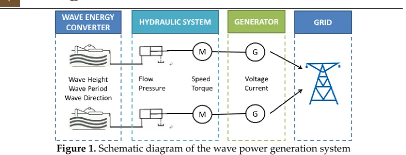
So far, more than 1,000 WECs have been patented worldwide, which can be classified into three categories [5]: OWC devices [6], oscillating body systems [7], and overtopping converters [8]. Among them, a mechanical interface is required to convert the intermittent multi-direction motion into a continuous one-direction motion and the hydraulic motors represent one of the most frequently equipped transmissions in the oscillating body systems [10]. The schematic diagram of a typical hydraulic oscillating body system is shown in Figure 1. A WEC is typically formed by three stages when converting wave energy to electrical energy. This includes (a) a front interface, the portion of a device that directly interacts with the incident waves, (b) a PTO system used to transform the front-end energy into other forms of energy, like mechanical energy, and (c) an electrical energy generation system that takes the responsibility to do the final conversion [3]. In the wind energy industry, the SCADA system, which records hundreds of variables related to operational parameters, is installed in most modern wind farms [11]. Compared with wind turbines, the data available from WECs are not as abundant in quantity because of the presently immature ocean wave technologies. However, it is worth mentioning that acquiring data from the operating WECs is more difficult than the wind turbines because of not only the harsh ocean conditions but also the high cost.
3
Figure 1. Schematic diagram of the wave power generation system
Traditionally, wave height and direction can be forecasted by both statistical techniques or physics-based models [13], [14]. There are many examples of the wave forecast system based on physical models. For example, the ECMWF and the WAVEWATCH-III organizations have performed predictions using wind data from the GDAS, Ocean weather and Gulf of Mexico [15]. The statistical approaches such as neural networks and regression-based techniques have also made great progresses [16][17]. By contrast, the physics-based wave forecasting models are widely used due to the mature technology and adequate historical data. The wave prediction can take advantage of opportunities from rapid development in recent years in the wind power prediction. Many algorithms, approaches and methods have been developed in the domain of statistical models in the renewable energy prediction, such as wind power and solar power prediction. So far, ANN methodology has been applied to predict short–mid-term solar power for a 750 W solar PV panel [20]. A LS SVM based model was applied for short-term forecasting of the atmospheric transmissivity, thus determining the magnitude of solar power [21]. The very short-term wind power predictions problems were addressed in the wind power industry by developing the NN model and the SVM, boosting tree, random forest, k-nearest neighbour algorithms [18], [19]. The data-based models with wind speed, wind generator speed, voltage and current in all phases as inputs could achieve an accurate prediction of the wind power output [22]. For medium-term and long-term wind power prediction, ANN models, adaptive fuzzy logistic and multilayer perceptrons are the most popular kinds of methods [23]-[25]. Moreover, as the deep learning algorithms bloom, the CNN, LSTM, DBN and RNN modelling have become popular in some renewable energy predictions. A deep RNN was modelled to forecast the short-term electricity load at different levels of the power systems. Deep multi-layered neural model has been reported to evaluate the electricity generation output from a wind farm 1 day in advance. A novel hybrid deep-learning network associated with an empirical wavelet transformation and two kinds of RNN was employed to make the accurate prediction of the wind speed and wind energy [26]- [28].
The primary intention of this work is to illustrate the power prediction and performance of a hydraulic WEC operating in the open sea condition for more than two months based on statistical analysis and physical modelling technologies. A multi-input approach based on CNN is presented to predict the power output at a particular coastal area. The CNN network reaches considerable achievement in terms of image and video recognition as well as language processing. One of the novelties is that the algorithms capable of converting the multi-input time series data into 2D images play a unique role in the construction of CNN model. The performance turns out to be remarkably better than other models, indicating its strong feasibility and suitability for power prediction. In addition, the connection between converter, hydraulic system, generator, and the grid will be clarified through analysing the wave, hydraulic motor pressure, and electrical data.
4
Section 3 describes the methodology of CNN algorithm in details. In Section 4, performance and results of the proposed model are presented. Finally, Section 5 summarizes the conclusions from the study.
2. Operation and performance analysis
2.1 Data acquisition
Normally, there are three conversion stages to extract wave energy from the ocean. This includes (a) capture of the kinetic energy by the power capture system of WEC, (b) conversions to the mechanical energy by PTO and then to the electrical power by generators, such as direct-drive linear generators; (c) storing of the electricity into batteries or transport to grid Error!
Reference source not found.. The data used in this study were acquired from a demonstrating
WEC deployed in open sea condition in a near-shore area. The principle of this WEC contains a double-buoy hydraulic OBD with ten kW level capacity with a time duration from February to April 2017. As shown in Figure 2, the WEC contains an oscillating buoy system and comprises of four main parts, i.e., power capture, hydraulic motor, generator and power transmission. The oscillating buoy captures kinetic energy through its up-and-down motions of the ocean waves. The hydraulic motor and generator take the responsibility to convert the kinetic energy into electricity and transfer to land through sea cable. In the first conversion, the wave energy is captured by two oscillating buoys while a hydraulic pressure system is deployed in the second conversion. The power capture system uses hydraulic rams installed inside of the two oscillating buoys. This 10 kW WEC prototype was invented by a research institution in 2016 and made the first sea testing at a testing station in SanYa, Hainan Province, China in 2017. The two oscillating buoys were installed on the edge of a dock side by side that were fixed together and moved up and down simultaneously along with the wave climate. The wave condition in this area changes significantly during seasons. The simulating data from numerical model show that the mean wave height reaches 0.7 m in summer with major south direction. The wave height in winter is much higher than summer, with 2.0 m maximum height and northeast direction [29]. The real wave heights are observed by an optical wave meter and recorded every 4 hours from 8:00 to 18:00 daily from February to April 2017. The real data show the maximum wave height is approximately 1.1 m during the observation period.
Figure 2. Schematic diagram of the hydraulic oscillating body system
5
is inactive. These occasions may be caused by the periods of low wave energy and harsh condition; some abnormal values within the data caused by disturbing signals and power failure also need to remove. Figure 3 shows the measurement data of these four variables after pre-processing.
Figure 3. Examples of pre-processed data measured from the WEC
2.2 Power curves
The extraction energy efficiency of wave energy varies wildly with different WECs because of the individual extents of technologies. Typically, the extraction energy efficiency between wave resource and hydraulic system can be calculated by dividing wave resource with powers achieved by the hydraulic system, which depends on the level of maturity of devices. The wave resource can be calculated by the equation below:
𝑃𝑟𝑒𝑠 =
1
8𝜌𝑔𝐻
2𝐶
𝑔 (1)
where 𝑃𝑟𝑒𝑠 stands for the power input from wave power, 𝜌 stands for the density of sea
water, 𝑔 stands for theacceleration of gravity, 𝐻 stands for the wave height and 𝐶𝑔 stands
for the group velocity. The group velocity can be calculated by the equation below:
𝐶𝑔=
1
2(1 +
2𝑘ℎ
𝑠𝑖𝑛ℎ (2𝑘ℎ))
𝐿
𝑇 (2)
where h stands for the waver height, L stands for the wave length, 𝑇 stands for the wave period and 𝑘 = 2𝜋/𝐿 stands for numbers of wave [30].
The input and output power of the hydraulic system can be calculated by the equation 3 and 4 respectively:
𝑃𝑡= 𝑝𝑟𝑒 × 𝑄 (3)
where 𝑃𝑡 stands for the input power of the hydraulic system; 𝑝𝑟𝑒 stands for pressure
and 𝑄 stands for the flow.
𝑃 =𝑀 × 𝑛
9550 (4)
where 𝑃 stands for the power output of the hydraulic system; 𝑀 stands for torque and 𝑛 stands for speed.
[image:5.595.157.424.132.356.2]6
height and active power output from the hydraulic system, as illustrated in Figure 4. These green dots denote the input power while the blue dots represent the power output. It can be observed that both power input and output tend to keep a positive correlation with the wave height when it is higher than 0.2 m. The positive correlation diverges from each other when the wave height is higher than 0.6 m. In general, these trends coincide with calculations from the equation of wave energy ([31]) that varies with the square of wave height. It can also be seen that the device is kept inactive when the wave height is below approximately 0.25 m, indicating the start wave height of this device is 0.25 m. When compared between these two power curves, it is found that the efficiency from wave energy to hydraulic power output have the little difference between 0.2 m and 0.6 m. Nevertheless, it increases smoothly with increasing of the wave height when higher than 0.6 m; this could reveal the mechanism of input and output power efficiency of this particular device.
Figure 4. Comparison of the input and output power of the hydraulic system
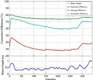
2.3 Energy conversion efficiency
The efficiency of a PTO system is vital to determine the stability and reliability of the device. Of the current WEC concepts developed so far, 42% use hydraulic systems to increase the overall efficiency of the converters and the electric performance [32]. For this WEC, the efficiencies from three parts, i.e., hydraulic system, electrical generator and electricity storage, were evaluated using historical data. The data were averaged every 4 hours for an entire day of 24 hours (6 groups’ data each day). The average efficiency of the hydraulic system Ef is
calculated by P P⁄ t. Here, P represents the average conversion efficiency from the power input
while Pt represents the average conversion efficiency from the power generation.
[image:6.595.145.477.242.479.2]7
direction also causes variation of the energy efficiency because the geographic terrain and conditions can amplify the wave height and concentrate wave energy on a particular position [33]. The curves also give the information that the generating conversion has the greatest potential for improvement.
Figure 5. The comparison of different conversion efficiencies from the hydraulic system,
electrical generator and electricity storage
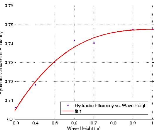
[image:7.595.136.443.138.402.2]8
Figure 6. The wave height –hydraulic conversion efficiency curve of this WEC
3. Methodology
3.1 Convolutional Neural Networks
Due to the 1D time series data from WEC may ignore vital information between time intervals, we applied a novel CNN algorithm, which convert 1D input data into 2D images. Traditionally, AM, LDS, and the popular HMM represent the classic approaches for modelling sequential time series data. The parameters to be predicted are used as perceptual judgements and features to do the classification [34]. However, deep learning, which is derives from ML is able to learn high-level abstractions in data by utilizing hierarchical architectures [35]. As one of the deep learning algorithms, CNN method has been considered one of the most appropriate methods to address the predicting problems. It has addressed plenty of problems in terms of sequential learning and shown its great potential in recent years [36]. The input and output data of the network observed in this paper is considered as a multiple data source, showing the connections between different parts of the device. The wave represents the original driver of the whole generation system, which could not be predicted accurately. This novel CNN approach shows advantages on prediction of the physical variables and makes considerable improvements in terms of the standard deviation and mean absolute values of the prediction performance. It also outperforms ML by a significant forecasting stability and accuracy.
[image:8.595.170.438.86.308.2]9 3.2 Network Architecture
[image:9.595.109.508.286.533.2]This network structure is formed by four hidden layers and the relevant hyper-parameters are shown in Figure 7. The values of the hyper-parameters used in the network are listed in Table 1. The input layer is four time series of observations collected from the hydraulic system of a WEC. The 1D to 2D conversion layer is used to rearrange one image set by the four series of observations mentioned in Section 2.1. The size of input layer is set to 28 × 28 pixels because 28 pixels are the default value of digital image in traditional CNN. The convolution layer performs convolution operations with the kernel size of 5×5 to acquire feature maps of the image. The dimension of the first convolution layer is set as 24 × 24 × 25, which convolutes an input image size from 28 × 28 pixels (25 layers set by experience). All the convolution layers are connected to the ReLU activation functions instead of sigmoid function because ReLU is faster and can reduce likelihood of vanishing gradient [41]. We use the max-pooling layer 2 × 2 and second convolution layers (5×5 kernel size and 25 layers as well). Finally, the dimension of the fully connected layer is set as 40, followed by a predict layer as required.
[image:9.595.185.411.579.687.2]Figure 7 The fundamental structure of the CNN
Table 1. List of the values of hyper-parameters used in this network
Hyper Parameters Values
Input variables 4
CNN Layers 25
Fully Connected Layer 40
Predict Layer 1
Batch size 20
Number of Epochs 100
The activation function of the predict layer is a linear function (identity function, i.e., y = x) because the values are unbounded in terms of regression.
The CNN is trained using the least absolute deviations (L1) as the loss function to minimize the absolute differences between the jth target value 𝑑
0 (𝑗)
10
𝑆 = ∑ |𝑑0(𝑗)− 𝑑𝑡(𝑗)|
𝑛
𝑗=0
(5)
where n denotes the size of the dataset.
Convolution Layer:
The convolution layer is comprised from a two-layer feed-forward NN. The NN uses a convolution algorithm to extract the feature maps from original image [42]. As mentioned above, the neurons in the same layer have no connections. But the neurons in different layers are deployed in order to simplify the feed forward process, as well as back propagation. Noticeably, the weights and feature map are convolved in the previous layer. An activation function is used to generate the current layer and output feature maps. The convolution layer is calculated as follows,
𝑎𝑖,𝑗 = 𝑓 ( ∑ ∑ 𝑤𝑚,𝑛𝑥𝑖+𝑚,𝑗+𝑛+ 𝑤𝑏
2
𝑛=0 2
𝑚=0
) (6)
where xi,j denotes a specific element in the input image, wm,n denotes the weight in mth row nth column, wb represents bias of the filter, ai,j is the element of the feature map. Notice that the ReLU function is chosen as the output activation function f.
Pooling Layers:
Pooling layers are typically used immediately after convolution layers to simplify the information. Traditionally, convolution layers associate with pooling layers for the sake of constructing stable structures and preserving characteristics. Another advantage of applying pooling layers is that it is able to save modelling time remarkably. There are many pooling methods available such as max pooling and average pooling. We thus focus on average pooling, which in fact allows us to see the connection with multi-resolution analysis. Given an input x = (x0, x1, … , xn-1)∈Rn, average pooling outputs a vector of a fewer components y =(y0, y1, … , y m-1)∈Rm as
𝑦𝑗=
1
𝑝∑ 𝑥𝑝,𝑗+𝑘
𝑝−1
𝑘=0
(7)
where p defines the support of pooling and m = n/ p. For example, p = 2 means that we reduce the number of outputs to a half of the inputs by taking pair-wise averages.
Fully connected Layers:
Usually the fully connected layer is located at the last hidden layer of the CNN. It is a linear function and is able to concentrate all representations at the highest order into a single vector.
Specifically, it is easy to change the highest order representations, P ∈ ℝ𝐾ℎ×𝑑×𝑝for,
𝑃1ℎ, … , 𝑃𝐾ℎ
ℎ (𝑎𝑠𝑠𝑢𝑚𝑖𝑛𝑔 𝑃
𝑘ℎ ∈ ℝ𝑑×𝑝), into a vector, then convert it with a dense matrix H ∈
ℝ(𝐾ℎ×𝑑×𝑝)×𝑛and apply non-linear activation:
𝑥̂ = 𝛼(𝑝𝑇𝐻) (8)
where 𝑥̂ ∈ ℝ𝑛can be seen as the final extracted feature vector. The values in matrix H are
parameters optimized during training. The n denotes a hyper-parameter and the representation size of the model [43].
Predict Layers
Linear predict layers are used to forecast the final results after obtaining the feature vector 𝑥̂𝑖𝑟,
𝑦𝑖𝑟= [1, 𝑥̂𝑇] ∙ 𝑊 (9)
The values in vector w will be optimized during training.
Back propagation algorithm
11
The parameter weights and biases are often used in the CNN. The BP is able to minimize the residuals 𝐸𝑚 between the prediction and the target using following equation,
𝐸𝑚=
1
𝑚∑ ∑(ℎ𝑗
𝑖− 𝑦
𝑗𝑖) 2 𝑑 𝑗=1 𝑚 𝑖=1 (10)
where 𝐸𝑚 represents squared-error loss function. The weights W and different biases b, β, c can be undated using following rules,
𝑊 = 𝑊 − 𝜂 ∙ 𝜕𝐸𝑚/𝜕𝑊 (11)
𝑏 = 𝑏 − 𝜂 ∙ 𝜕𝐸𝑚/𝜕𝑏 (12)
𝛽 = 𝛽 − 𝜂 ∙ 𝜕𝐸𝑚/𝜕𝛽 (13)
𝑐 = 𝑐 − 𝜂 ∙ 𝜕𝐸𝑚/𝜕𝑐 (14)
here, ∂Em/ ∂W, ∂Em/ ∂b, ∂Em/ ∂β and ∂Em/ ∂c represent the partial derivatives of the
loss function in terms of W, b, β and c.
3.3 Model Performance Metrics
Three mainstream performance metrics are considered here to evaluate the accuracy of forecasting, which are RMSE, the MAE and the R2. For the RMSE, it is more sensitive to a large deviation between the forecasted values and the actual values. The MAE, on the other side, performs the absolute difference value between the forecasts and the actual values. The MAE also describes the magnitude of an error from the forecast on average. RMSE and MAE are calculated by Equation 15-17.
𝑅𝑀𝑆𝐸 = 1
√𝑁√∑(𝐼(𝑝𝑟𝑒𝑑,𝑖)− 𝐼𝑚𝑒𝑎𝑠,𝑖)
2 𝑁
𝑖=1
(15)
𝑀𝐴𝐸 =1
𝑁∑|𝐼(𝑝𝑟𝑒𝑑,𝑖)− 𝐼𝑚𝑒𝑎𝑠,𝑖|
𝑁
𝐼=1
(16)
Here the coefficient of determination is employed to optimize the appropriate model structure,calculated as follows,
𝑅𝑇2 = 1 −
𝜎𝑒2
𝜎𝑦2 (17)
where 𝜎𝑒2 denotes the variance of the residuals between model predict and the actual
output, also known as sample residuals and 𝜎𝑦2 denotes the variance of the actual output. It is
clear that the 𝑅𝑇2 becomes unity when the residuals turn into low values, meaning the network
presents a considerable performance of the actual output. By contrast, when the 𝑅𝑇2 tends to
zero, it means the variances become similar, thus elaborating an inappropriate fit [44].
4. Results and Discussions
4.1 Dataset
12
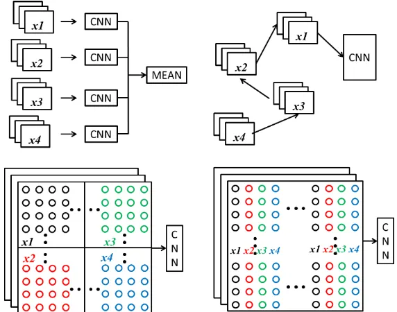
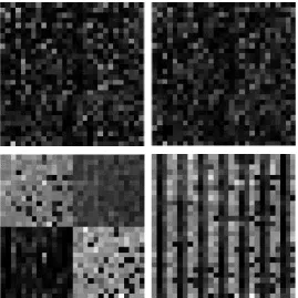
[image:12.595.158.444.232.457.2]The data used in the CNN include four sequential inputs and one output. Four parameters (hydraulic pressure, hydraulic flow, motor speed and motor torque) from the hydraulic system are taken as the inputs of the CNN and the power generation is the output of the network. Here, the total 100,352 samples acquired from February to April 2017 are sequentially separated into 80,281 as the training dataset (80%), 5,019 as the validation dataset (5%) and 15,052 as the test dataset (15%). Firstly, the four time series inputs should be rearranged to a 2D image before applying CNN for regression and prediction. Four different conversion methods are attempted to achieve a better training accuracy, including (a) results averaged by the individual CNN of the four inputs; (b) four inputs sequentially rearranged before training; (c) a single 2D image being divided into four sub-images formed by four inputs respectively; (d) an image rearranged by four inputs in sequence, as shown in Figure 8.
Figure 8 Dataset conversion methods, top left: four inputs applied to the model respectively,
top right: four inputs applied to the model sequentially, the bottom ones: four inputs rearranged to the image respectively and sequentially
4.2 Results
This section introduces the results of evaluation of the wave power generation prediction model. Different proposed patterns converted from inputs by various methods are compared firstly. Different input image sizes (28×28, 20×20, 14×14, 10×10 pixels) are deployed to discuss how image size could affect the forecasting results. Curve fitting plots from each conversion method are presented for the sake of revealing fitting details. In order to demonstrate the superiority of the methods, the CNN model is employed along with different mainstream supervised modelling approaches, such as ANN, SVM, LR and RT. Finally, the RMSE, MAE and R2 are used as the metrics to evaluate the prediction performance from multiple criteria perspectives.
13
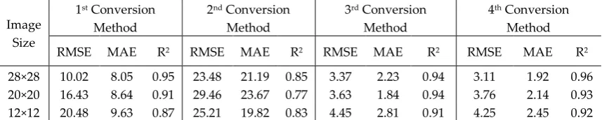
[image:13.595.84.513.144.230.2]4th conversion methods obtain lower RMSE and MAE values and a higher R2 value. The forecast from the 2nd method represents the poorest fit with these raw data.
Table 2.Prediction performance of the CNN model through different image sizes and
methods
Image Size
1st Conversion
Method
2nd Conversion
Method
3rd Conversion
Method
4th Conversion
Method
RMSE MAE R2 RMSE MAE R2 RMSE MAE R2 RMSE MAE R2
28×28 10.02 8.05 0.95 23.48 21.19 0.85 3.37 2.23 0.94 3.11 1.92 0.96
20×20 16.43 8.64 0.91 29.46 23.67 0.77 3.63 1.84 0.94 3.76 2.14 0.93
12×12 20.48 9.63 0.87 25.21 19.82 0.83 4.45 2.81 0.91 4.25 2.45 0.92
The four plots shown in Figure 9 demonstrate the result as well. The predicting curves fit the real output well in all the four plots except the top right one that represents the 2nd conversion method. In the top left subplot, the two curves fit much better in high power level than in low level. The bottom subplots perform both remarkable fitting results when forecasting these distinctive fluctuations. The results also illustrate that similar characteristics are extracted from images created by the different data arrange algorithms. Clearly, the top right subplot obtained with the 2nd conversion method, i.e., four inputs applied to the model respectively, exhibits poor fitting in both high and low power levels.
Figure 10 illustrates 2D images of the network input converted from time series 1D inputs.
14
Figure 9 The comparison of the prediction results from different conversion methods based
on 28×28 dimension image, with 1st to 4th conversion method being presented from top left to right bottom subplot
[image:14.595.166.436.473.743.2]15
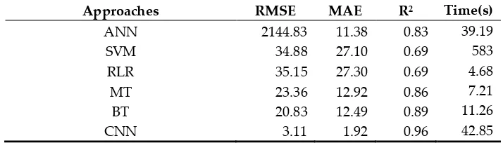
Table 3. The performance of CNN compared with different supervised modelling approaches
(28×28 dimension size)
Approaches RMSE MAE R2 Time(s)
ANN 2144.83 11.38 0.83 39.19
SVM 34.88 27.10 0.69 583
RLR 35.15 27.30 0.69 4.68
MT 23.36 12.92 0.86 7.21
BT 20.83 12.49 0.89 11.26
CNN 3.11 1.92 0.96 42.85
4.3 Discussions
In terms of validation and accuracy, different supervised modelling approaches are applied for comparison, and the results are shown in Table 3. This work was implemented based on a Xeon E3-1271 CPU with 3.6 GHz and 16 GB RAM workstation. The training time for the MCNN was compared with that taken for ML algorithms mentioned above. The SVM takes on an average of 583 s, which means the longest time among them. The CNN algorithm trains no more than 43 s if using the hyper-parameters in Table 1. The MT and BT got an average of 7.21 s and 11.26 s respectively, almost four times faster than the CNN. This indicates that the CNN model provides much higher accuracy even a little longer time consumed than the ML algorithms.
Table 3 also provides sufficient evidence that CNN made considerable achievement in wave power prediction among these ML algorithms. The indicators of the difference between actual and forecast values become quite small if the CNN model is used. SVM and RLR produce the worst performance as the MAE value is much higher (more than twice than others) among the five models, which mean these performance measures are much bigger and the error can be easily expected from the forecast. The R2 values of ANN, MT and BT show general fitting results. It is worth mentioning that the training of ANN and CNN take a little longer time (more than 43 s in this situation) and the time greatly depends on hidden layers, epochs and break time of the network.
It is known that the form of data modelled in CNN is widely applied in 2D image, which includes connection from neighbourhood [47]. The more features captured from the training images, the better performance provided by the model. The four patterns of image (data arrangement) trained in the different CNN models show the distinctive features contained in images. The large size of images contains more features than the small size ones. The prediction is affected by not only the current inputs but also the connections in the same input series and the adjacent input series in between. In other words, the current inputs combined with adjacent pixels could provide more information than a single input. Let’s take the 4th conversion method as an example, in time t, the 𝑥2𝑡 is affected by 𝑥2𝑡−1, 𝑥2𝑡+1 and 𝑥1𝑡, 𝑥3𝑡, as shown in Figure 11.
16
In addition, the number of the convolution layers and feature extractor layers also need to be discussed. It seems that increasing the number of feature maps and convolution layers could improve the accuracy of the model; but actually it works in many conditions. We attempted to increase the number of the convolution layer and pooling layer from 1 to 3 and the feature map from 10 to 100. The neurons for the fully connected layer also increased from 10 to 100, and the number of layers increased from 1 to 3. Eventually, the training model consumed much more time, though the anticipated results did not appear to be much improved compared with the initial architecture. Consequently, we consider the architecture used in this article is superior enough for training and predicting such a complex problem.
Furthermore, the residual between actual and practical values is supposed to be a function of the inputs. The result is able to perform an early warning to indicate the possible appearance of the anomalies if the residual exceeds a predefined threshold. Thus, this MCNN model could perform condition monitoring and fault diagnosis for the ocean energy systems.
5. Conclusions
In this paper, the power characteristics of a double-buoy oscillating body WEC is presented by analysing the open sea testing data. The wave-power curve and the efficiencies of the hydraulic system are investigated to elaborate the connection between wave height and instantaneous power output of the WEC. A convolutional neural network with multiple inputs has been developed for predicting the power output of the near-shore WEC. It uses four hydraulic system parameters as inputs, i.e., hydraulic pressure, hydraulic flow, motor speed and motor torque, and the power output as output. The proposed CNN applies 1D to 2D data conversion to convert time series data into image data..
This result shows that the MCNN performs much better predicting results compared with other mainstream supervised modelling approaches, such as ANN, SVM, LR and RT, with the highest R2 value being achieved 0.96. It can also be found that both the image size and the conversion method can affect the results. The intersectional methods for data conversion with a larger dataset size can capture more features from the training images, thus providing a better performance for the model fitting. The proposed MCNN is therefore feasible enough for training and predicting the power output from a complex system such as the WEC studied in this paper based on the experimental data.
Besides the time-domain analysis, time-frequency analysis using wavelet transform has also been attempted based on the same data [48], [49], the results were found to be widely divergent, and further work will be performed in the near future. Nevertheless, this work makes progress on managing the power generation, transformation and storage of a WEC system for ocean renewable energy systems.
Acknowledgments
This research is supported by CSC (Chinese Scholarship Council) and the Engineering Department at Lancaster University, UK.. Some of the work received support from SFMRE (Special Funds for Marine Renewable Energy) from SOA (Grant number GHME2017ZC01).
Reference
[1] Y. Saadat, Nelson Fernandez, Alexei Samimi, Mohammad Reza Alam, Mostafa Shakeri, Reza Ghorbani. Investigating of Helmholtz wave energy converter. Renewable Energy 87 (2016) 67-76 [2] Shangyan Zou, Ossama Abdelkhalik, Rush Robinett, Giorgio Bacelli, David Wilson. Optimal control
of wave energy converters. Renewable Energy 103 (2017) 217-225
17
front end conversion in ocean wave energy Converters. Front. Energy 2015, 9(3): 297–310
[4] Davide Magagna, Riccardo Monfardini, Andreas Uihlein. JRC Ocean Energy Status Report 2016 Edition. Luxembourg: Publications Office of the European Union, 2016
[5] A. F. de O. Falcao, Wave energy utilization: a review of the technologies. Renew and Sustainable Energy Review. 14 (3) (2010) 899-918
[6] M.-F. Hsieh, I.-H. Lin, D. Dorrell, M.-J. Hsieh, C.-C. Lin. Development of a wave energy converter using a two chamber oscillating water column. Sustain.Energy IEEE Trans. 3 (3) (2012) 482-497 [7] A. Sproul, N. Weise, Analysis of a wave front parallel WEC prototype, Sustain. Energy IEEE Trans.
6 (4) (2015) 1183-1189
[8] Contestabile P., Iuppa C., Di Lauro E., Cavallaro, L. Andersen T.L., Vicinanza D. Wave loadings acting on innovative rubble mound breakwater for overtopping wave energy conversion. Coastal
Engineering, Volume 122, April 2017, Pages 60-74, ISSN 0378-3839,
http://dx.doi.org/10.1016/j.coastaleng.2017.02.001.
[9] Buccino, M., Vicinanza, D., Salerno, D., Banfi, D., & Calabrese, M. Nature and magnitude of wave loadings at seawave slot-cone generators. Ocean Engineering, 95, 34-58.
[10] Anto´nio F. de O. Falca˜o. Wave energy utilization: A review of the technologies. Renewable and Sustainable Energy Reviews 14 (2010) 899–918
[11] Wenna Zhang, Xiandong Ma. Simultaneous Fault Detection and Sensor Selection for Condition Monitoring of Wind Turbines. Energies 2016, 9, 280
[12] Fuat Kara. Time domain prediction of power absorption from ocean waves with wave energy converter arrays. Renewable Energy 92 (2016) 30-46
[13] Reikard G, Pinson P, Bidlot J-R. Forecasting ocean wave energy: the ECMWF wave model and time series methods. Ocean Eng 2011; 38:1089–99. http://dx.doi.org/10.1016/j.oceaneng.2011.04.009. [14] Reikard G. Integrating wave energy into the power grid: simulation and forecasting. Ocean Eng
2013; 73: 168–78. http://dx.doi.org/10.1016/j.oceaneng.2013.08.005.
[15] Andreas Uihlein, Davide Magagna. Wave and tidal current energy- A review of the current state of research beyond technology. Renewable and Sustainable Energy Reviews 58 (2016)1070–1081 [16] Eikard G. Integrating wave energy into the power grid: simulation and forecasting. Ocean Eng 2013;
73:168–78. http://dx.doi.org/10.1016/j.oceaneng.2013.08.005.
[17] Malmberg A, Holst U, Holst J. Forecasting near-surface ocean winds with Kalman filter techniques. Ocean Eng 2005; 32:273–91. http://dx.doi.org/10.1016/j.oceaneng.2004.08.005.
[18] Peres, D. J., Iuppa, C., Cavallaro, L., Cancelliere, A., & Foti, E. (2015). Significant wave height record extension by neural networks and reanalysis wind data. Ocean Modelling, 94, 128-140. doi:10.1016/j.ocemod.2015.08.002
[19] James, S. C., Zhang, Y., & O'Donncha, F. (2018). A machine learning framework to forecast wave conditions. Coastal Engineering, 137, 1-10. doi:10.1016/j.coastaleng.2018.03.004
[20] Ercan Izgi, Ahmet Oztopal, Bihter Yerli. Short–mid-term solar power prediction by using artificial neural networks. Solar Energy 86 (2012) 725–733
[21] Jianwu Zeng, Wei Qiao. Short-term solar power prediction using a support vector machine. Renewable Energy 52 (2013) 118-127
[22] Vargas L, Paredes G, Bustos G. Data mining techniques for very short term prediction of wind power. IREP Symposium-Bulk Power System Dynamics and Control-VIII; 2010:1-7.
[23] Ilhami Colak, Seref Sagiroglu, Mehmet Yesilbudak. Data mining and wind power prediction: A literature review. Renewable Energy 46 (2012) 241-247
[24] Makarynskyy, et al. Filling gaps in wave records with artificial neural networks, Maritime Transportation and Exploitation of Ocean and Coastal Resources, Vols 1 and 2 Pages: 1085-1091, 2005.
[25] Ciortan, S., Rusu, E., Prediction of the wave power in the Black Sea based on wind speed using artificial neural networks, International Conference on advances in Clean Energy Research, ICACER 2018, Barcelona, Spain 6-8 April, 2018
[26] J. M. Torres, R. M. Aguilar, K. V. Zu niga-Meneses. Deep learning to predict the generation of a wind farm. JOURNAL OF RENEWABLE AND SUSTAINABLE ENERGY 10, 013305 (2018)
18
empirical wavelet transform, long short term memory neural network and Elman neural network. Energy Conversion and Management 156 (2018) 498–514
[28] Heng Shi, MingHao Xu, Qiuyang Ma, Chi Zhang. A Whole System Assessment of Novel Deep Learning Approach on Short-Term Load Forecasting. 9th International Conference on Applied
Energy, ICAE2017, 21-24 August 2017, Cardiff, UKWikipedia.
https://en.wikipedia.org/wiki/Expected_value#cite_note-Ross-1
[29] Yi Z. Wind and Wave Analysis of QingShui Bay Based on WRF and SWAN Model.
http://www.docin.com/p-1440602358.html
[30]C Ni, H Wu, R Zhang. The Technical Development and Demonstration of Marine Energy in China. 2018, Tianjin China. Tianjin Science and Technology Press.
[31] Jinjiang Wang, Yulin Ma, Laibin Zhang, Robert X. Gao, Dazhong Wu. Deep learning for smart manufacturing: Methods and applications. Journal of Manufacturing Systems xxx (2018) xxx– xxx(article in press)
[32] Ruud Kempener (IRENA), Frank Neumann (IMIEU). Wave Energy Technology Brief. International Renewable Energy Agency. 2014
[33] Zhipeng Zang, Qinghe Zhang, Yue Qi, Xiaoying Fu. Hydrodynamic responses and efficiency analyses of a heaving-buoy wave energy converter with PTO damping in regular and irregular waves. Renewable Energy 116 (2018) 527-542
[34] G.W. Taylor, Composable, distributed-state models for high-dimensional time series (Ph.D. thesis), Department of Computer Science, University of Toronto, 2009.
[35] YanmingGuo, YuLiu, ArdOerlemans, SongyangLao, SongWu, MichaelS.Lew. Deep learning for visual understanding: A review. Neurocomputing187(2016)27–48
[36] Graves, A., Supervised Sequence Labelling. Springer, 2012. pp. 5–13. Online:
http://link.springer.com/10.1007/978-3-642-24797-2_2
[37] Alberto Mozo, Bruno Ordozgoiti, Sandra GoÂmez-Canaval. Forecasting short-term data center
network traffic load with convolutional neural networks.
https://doi.org/10.1371/journal.pone.0191939. February 6, 2018
[38] Tomoyoshi Shimobaba, Takashi Kakue, Tomoyoshi Ito. Convolutional neural network-based regression for depth prediction in digital holography. https://arxiv.org/abs/1802.00664 . Feb 2018 [39] Dewi Suryani, Patrick Doetsch, Hermann Ney. On the Benefits of Convolutional Neural Network
Combinations in Offline Handwriting Recognition.
https://www-i6.informatik.rwth-aachen.de/publications/download/1021/Suryani-ICFHR-2016.pdf
[40] Wikipedia. Convolutional neural network.
https://en.wikipedia.org/wiki/Convolutional_neural_network#Distinguishing_features
[41] What are the advantages of ReLU over sigmoid function in deep neural networks. Stackexchange. https://stats.stackexchange.com/questions/126238/what-are-the-advantages-of-relu-over-sigmoid-function-in-deep-neural-networks
[42] Huai-zhi Wang, Gang-qiang Li, Gui-bin Wang. Deep learning based ensemble approach for probabilistic wind power forecasting. Applied Energy 188 (2017) 56–70
[43] Kui Zhao, Can Wang. Sales Forecast in E-commerce using Convolutional Neural Network. https://arxiv.org/abs/1708.07946
[44] Philip Cross, Xiandong Ma. Nonlinear system identification for model-based condition monitoring of wind turbines. Renewable Energy 71 (2014) 166-175
[45] Brian D. Ripley. Pattern Recognition and Neural Networks. Cambridge University Press; 1 edition (10 Jan. 2008)
[46] Stephen Johnson. Stephen Johnson on Digital Photography. O'Reilly. 0-596-52370-X,2006
[47] Anwen Zhu, Xiaohui Li, Zhiyong Mo, Huaren Wu. Wind Power Prediction Based on a Convolutional Neural Network. 2017 International Conference on Circuits, Devices and Systems [48] Shin Fujieda, Kohei Takayama, Toshiya Hachisuka. Wavelet Convolutional Neural Networks for
Texture Classification. arXiv:1707.07394v1 [cs.CV] 24 Jul 2017
[49] ROBI POLIKAR. THE WAVELET TUTORIAL SECOND EDITION PART I.