DOI: 10.1002/sim.8194
R E S E A R C H A R T I C L E
To add or not to add a new treatment arm to a multiarm
study: A decision-theoretic framework
Kim May Lee
1James Wason
1,2Nigel Stallard
31MRC Biostatistics Unit, University of
Cambridge, Cambridge, UK
2Institute of Health and Society, Newcastle
University, Newcastle upon Tyne, UK
3WMS - Statistics and Epidemiology,
University of Warwick, Coventry, UK
Correspondence
Kim May Lee, MRC Biostatistics Unit, University of Cambridge, Cambridge CB2 0SR, UK.
Email: [email protected]
Present Address
Kim May Lee, MRC Biostatistics Unit, School of Clinical Medicine, University of Cambridge, Cambridge CB2 0SR, UK.
Funding information
Medical Research Council, Grant/Award Number: MR/N028171/1 and
MC_UP_1302/4
Multiarm clinical trials, which compare several experimental treatments against control, are frequently recommended due to their efficiency gain. In practise, all potential treatments may not be ready to be tested in a phase II/III trial at the same time. It has become appealing to allow new treatment arms to be added into on-going clinical trials using a “platform” trial approach. To the best of our knowledge, many aspects of when to add arms to an existing trial have not been explored in the literature. Most works on adding arm(s) assume that a new arm is opened whenever a new treatment becomes available. This strat-egy may prolong the overall duration of a study or cause reduction in marginal power for each hypothesis if the adaptation is not well accommodated. Within a two-stage trial setting, we propose a decision-theoretic framework to investi-gate when to add or not to add a new treatment arm based on the observed stage one treatment responses. To account for different prospect of multiarm studies, we define utility in two different ways; one for a trial that aims to maximise the number of rejected hypotheses; the other for a trial that would declare a success when at least one hypothesis is rejected from the study. Our framework shows that it is not always optimal to add a new treatment arm to an existing trial. We illustrate a case study by considering a completed trial on knee osteoarthritis.
K E Y WO R D S
adding-arm, disjunctive power, multiarm, number of rejected hypotheses
1
I N T RO D U CT I O N
In recent years, a multiarm multistage design is becoming an attractive alternative to the classical randomised treatment-control design, especially in phase II and phase III trial settings. A multiarm multistage design has attractive features such as sharing a common control group in a study that investigates multiple treatment interventions concur-rently and allowing use of an adaptive design to drop arms for futility and efficacy at interim analyses. Another potential feature of a multiarm multistage design is to consider adding new treatment arm(s) to an on-going study, known as a plat-form trial. Apart from the benefit of sharing the concurrent control group, adding new treatment arm(s) provides extra treatment option(s) to future patients who are yet to be enrolled to the trial. This adaptive feature also enhances future patient benefit as the newly available agents could be tested immediately in the trial when they are available. Moreover, the overall cost of studying a new treatment intervention would be reduced as the cost of setting up an independent trial
. . . .
This is an open access article under the terms of the Creative Commons Attribution License, which permits use, distribution, and reproduction in any medium, provided the original work is properly cited.
© 2019 The Authors.Statistics in MedicinePublished by John Wiley & Sons Ltd.
can be avoided when the new agent can be tested in an on-going trial. Examples of on-going trials that consider the feature of adding new treatment arm(s) include STAMPEDE,1I-spy 2,2and Glioblastoma (GBM) AGILE.3
To date, limited statistical literature on methodology for adding arms is available. Cohen et al4provided a review of
papers discussing methodology and practical considerations for adding arms to an on-going clinical trial. With the deci-sion that a newly available treatment is always added to an on-going trial, Elm et al5compared three analysis approaches
based on the operating characteristics of the trial, which originally has a standard two-arm design. Restricting a fixed max-imum number of arms that can be added to a study, Ventz et al6illustrated the benefits of a rolling-arms design, which
is a specific platform design that adds new arms to a study when they become available. On other aspects, Ventz et al7
investigated three randomisation procedures for the design that adds new arms at different time points; Wason et al8
inves-tigated the impact of adding arms on family-wise error rate. We find that the exact time to open new arm(s) has not been well addressed by these authors. The strategy of always adding in the treatments once they become available may lead to having little power for each treatment or prolonging the overall duration of a study. On the contrary, being inflexible on including new treatments may result in missing the chance of identifying a truly effective treatment.
In the context of screening a large number of agents, Yuan et al9 proposed a platform trial design, whereby a new
treatment arm is opened once an experimental treatment graduates or is dropped. Focusing on futility monitoring, Hobbs et al10proposed a framework for designing a screening platform trial that could drop arms or add new agents using
Bayesian modelling. Here, we investigate the strategy of adding a new treatment to an existing study based on responses that are observed up to date. We focus on phase II/III setting where the objective of a trial is to study the efficacy of treat-ments. The situation we consider here is similar to those described in the works of Elm et al5and Ventz et al,6where a
new treatment becomes available after a trial on different interventions for the same disease has commenced but prior to the end of enrollment. Instead of following a stringent strategy, we investigate when would be best to add a new treatment arm to an on-going trial. To provide insight into how to decide whether to add a new treatment to an existing study, we consider a two-stage multiarm trial setting. We propose a decision-theoretic framework to provide guidance on when to add an arm to an on-going study based on the observed treatment responses to date.
A decision-theoretic approach explores the consequences of possible decisions and provides an optimal action that gives the highest gain on making a decision11-13; Hee et al14provided systematic review on decision-theoretic designs for clinical
trials. The notion of our framework is similar to the work of Berry and Ho,15who investigated stopping boundaries for
drug development programs. However, we consider a frequentist utility instead of a Bayesian one as the common practise of clinical studies emphasises the freqentist operating characteristic of the trial. For some common diseases, where many treatment options are available, a trial might be able to identify as many effective treatments as possible. In others, being able to identify one efficacious treatment from a study would be considered a success. To cover these different prospects, we consider two types of utility in this work: one depends on the number of rejected hypotheses, the other is a binary value that equals one when at least one hypothesis is rejected by the study. The expectation of the former corresponds to the expected number of rejected hypotheses, and of latter the disjunctive power when at least one of the rejected hypotheses are false under the null. They are examples of design criteria for designing a trial that has multiple clinical objectives.16
A utility function reflects the point of view of a decision marker. For ease of exposition, we do not include other trial aspects such as monetary values in our illustration. This may represent the interests of an academic trial sponsor who has limited budget for recruiting more patients but want to maximise the chance of declaring a trial success by adding a new treatment arm to an on-going trial. Other decision-makers such as trial sponsors and health regulators can incorporate the relevant aspects into the utility function and conduct the analysis described in this work.
The structure of this paper is as follows. In Section 2, we describe the background and key elements of our decision-theoretic framework. In Section 3, we illustrate the optimal decision that is made based on stage one responses for a case study of a trial in osteoarthritis,17and the impact of prior distribution on the optimal decision. In Section 4, we
illustrate the framework for an initial design that has (i) one treatment and a control arms, and (ii) two treatment and a control arms. In Section 5, we summarise our investigation, discuss the limitations of our work, and consider future work.
2
BAC KG RO U N D A N D D EC I S I O N-T H EO R ET I C F R A M E WO R K
first describe the trial setting and the distributions of the responses. We then present the analysis procedure to compute the probabilities of rejecting hypotheses based on a multivariate normal distribution prior to implementation of stage two of the trial. Following that, we specify the utility and describe the process of identifying the optimal decision, ie, to add or not to add a treatment arm to an on-going trial based on the observed stage one responses.
2.1
Distribution of data
Consider a two-stage multiarm trial that initially hasKtreatments and a control treatment, with a total sample size
N = N1 + N2, whereNsis stagessample size,s = 1,2. Denotek = 0 for a control treatment andk = 1,…,Kfor
experimental treatments. LetXkjbe the response of treatmentkon subjectj = 1,…,nks, wherenksis the sample size
of treatmentkfor stages,∑Kk=0nks = Nsandnk1 + nk2 = nk. Having observedN1 responses in stage one, we could
investigate the benefit of adding a new treatment arm, denoted byK+ 1, to the on-going study. A decision problem is to decide whether to add a new treatment and decide the value ofN2andnk2,k = 0,…,K+ 1 if armK+ 1 is added to the
trial. The value ofnK+ 1,2would depend on the randomisation procedure/scheme of the study; the value ofN2would affect
the power of making inference on treatmentK + 1. For ease of exposition, we restrictN2to be fixed in the illustration.
The case where additional patients are available if an arm is added is considered in the Discussion section. Following the decision to add an arm, we consider the use of an equal randomisation procedure such that each arm has stage two sample sizeN2∕(K+2). In other words, the decision of adding a new treatment arm would cause the initial arms to have a smaller stage-two sample size per arm.
Consider thatXkjare identically and independently normally distributed with mean𝜇k and variance𝜎k2, where𝜎k2is
a known value. Denote byX̄k.s =
∑nks
𝑗=1Xk𝑗 nks
the stagesmean response of treatmentk,X̄k = wk1X̄k.1+wk2X̄k.2as the mean
response of treatment k over both stages,wks = nnks k
. We haveX̄k.s iid
∼ N(𝜇k, 𝜎k2∕nks)andX̄k ∼ N(𝜇k, 𝜎k2∕nk). Without loss
of generality, consider a control treatmentk = 0 has𝜇0 = 0. Fork = 1,…,K,K + 1, let𝜇kfollow a normal prior
distribution with meanmk0and variancevk0. Prior to implementing the trial,X̄k.1has a prior predictive distribution that
follows a normal distribution with meanmk0 and variance 𝜎 2
k nk1
+vk0. Analogously, when treatmentK + 1 is added to
the trial at the end of stage one of the trial, the prior predictive distribution ofX̄K+1.2is a normal distribution with mean mK+ 1,0and variance 𝜎
2
K+1
nK+1,2
+vK+1,0.18
After observing stage one, the posterior distribution of𝜇khas mean
mk1= vk0
𝜎2
k nk1
+vk0 ̄ xk.1+
𝜎2
k nk1
𝜎2
k nk1
+vk0 mk0
and variance
vk1= (
1
vk0
+ nk1
𝜎2
k
)−1 ,
which become the prior moments for𝜇kof the next stage. The normal predictive distribution forX̄k.2has meanmk1and
variance𝜎
2
k nk2
+vk1.18Note thatmk1depends on stage one observation viax̄k.1. In what to follow, let𝑓̄xk.1(x̄k.1)and𝑓x̄k.2(x̄k.2|̄xk.1)
denote the (predictive) probability density function of stage one responses and of stage two responses. They are used in the computation of expectations.
2.2
Hypothesis testing
We now describe the analysis plan of the trial. Without loss of generality, positive values indicate that a treatment is more effective than a control treatment on the patients. Compare treatmentkwith the control treatmentk = 0, a hypothesis test considers
null hypothesis,H0k ∶ 𝜇k−𝜇0≤0,
At the end of the trial, we reject a hypothesisH0kwhen
(wk1X̄k.1+wk2X̄k.2) − (w01X0̄ .1+w02X0̄ .2) √
𝜎2
k nk1+nk2
+ 𝜎
2 0
n01+n02
>bk2.
When the null hypothesis is true, the left-hand side of the first expression is normally distributed with mean zero and variance one. To get a level𝛼test, we compare this test statistics to the rejection boundary,bk2 = Φ−1(1− 𝛼), whereΦ−1
denotes the cumulative density function of the standard normal distribution. In some trials withK > 1, it is desirable to control the family-wise type one error rate, ie, the probability of making at least one type one error is≤ 𝛼, or in the strong sense that this error rate is≤𝛼for any configuration of true and false null hypotheses. Methods such as Dunnett's test, Holm-Bonferroni method, and closed testing procedure are often used to control the error rate in multiarm multi-stage designs. Without loss of generality, we consider controlling the family-wise error rate in the strong sense. We use Bonferroni correction, ie, whenK > 1 hypotheses are tested by the study, we choosebk2 = Φ−1(1 − 𝛼∕K).
Since X̄k.s,k = 0,1,…,K, s = 1,2, are independent and normally distributed,wksX̄k.s are also independent and
normally distributed but with a variance scaled byw2
ks. It can be shown that the differences in mean response of treatments
for stage two given the stage one data follow a multivariate normal distribution, ie,
⎛ ⎜ ⎜ ⎜ ⎝
w12X̄1.2−w02X̄0.2 w22X̄2.2−w02X̄0.2
⋮
wK2X̄K.2−w02X0̄ .2 ⎞ ⎟ ⎟ ⎟ ⎠ ∼MVN ⎡ ⎢ ⎢ ⎢ ⎣ ⎛ ⎜ ⎜ ⎜ ⎝ m11 m21 ⋮ mK1
⎞ ⎟ ⎟ ⎟ ⎠ , diag ( w212
( 𝜎2
1 n12 +v11
)
,…,w2K2 (
𝜎2
K
nK2
+vK1 ))
+w202𝜎 2 0 n021K
⎤ ⎥ ⎥ ⎥ ⎦ ,
where1Kis a square matrix of ones with dimensionK. We can compute the probabilities of rejecting some hypotheses
by evaluating the cumulative density function of this distribution using some numerical software. For example, the probability of rejecting all hypotheses except hypothesisrand hypothesisuis
P(H0r andH0uare not rejected,H0l,l∈ {1,…,K}∖{r,u} are rejected)
=P[wr2X̄r.2−w02 X̄0.2≤Z(r,2), wu2X̄u.2−w02X̄0.2≤Z(u,2), wl2X̄l.2−w02X̄0.2 > Z(l,2),l∈ {1,…,K}∖{r,u}]
=∫ l1 ∫ l2 ∫ lK
f(x̄2)d(x̄2), (1)
wheref(x̄2)is the pdf of the multivariate normal distribution,Z(k,2) = bk2 √
𝜎2
k nk1+nk2 +
𝜎2 0
n01+n02 − (
wk1X̄k.1−w01X̄0.1),k =
1,…,K, andlkdenote the regions of the integrals;lk = [Z(k,2),∞)fork ∈ {1,…,K}∖{r,u}, andlk = ( −∞,Z(k,2)]
fork ∈ {r,u}. We consider thisK-dimensional joint distribution when we compute the expected utility of not adding an arm to an on-going trial.
Note that nonequalwks,k = 1,…,K, imply that the trial has different number of observations on different arms. This
could happen for example by design, ie, using unequal treatment allocation probabilities, or because of the presence of missing observations and/or delayed outcomes. With equal randomisation probability and fully observed responses that are available at the time of making a decision, we havewks = w0sfork = 1,…,K, ands = 1,2.
For the newly added arm, concurrent control responses are used in making inference and we rejectH0,K+ 1when
̄
XK+1.2−X0̄ .2>bK+1,2 √
𝜎2
K+1 nK+1,2
+ 𝜎
2 0 n02
.
To be consistent with the notation, we denoteZ(K + 1,2) = bK+1,2 √
𝜎2
K+1
nK+1,2
+ 𝜎02
n02
. Note that the joint distribution of
̄
thisK+1-dimensional multivariate normal distribution to compute the expected utility of adding an arm to an on-going trial, ie, ⎛ ⎜ ⎜ ⎜ ⎝
w12X̄1.2−w02X̄0.2 ⋮
wK2X̄K.2−w02X0̄ .2 ̄
XK+1,.2−X0̄ .2 ⎞ ⎟ ⎟ ⎟ ⎠ ∼MVN ⎡ ⎢ ⎢ ⎢ ⎣ ⎛ ⎜ ⎜ ⎜ ⎝ m11 ⋮ mK1 mK+1,0
⎞ ⎟ ⎟ ⎟ ⎠ , diag ( w212
( 𝜎2 1 n12 +v11 )
,…,w2K2 (
𝜎2
K
nK2
+vK1 )
, 𝜎 2
K+1 nK+1,2
+vK+1,0 ) +diag ( w2 02 𝜎2 0 n02,…,w
2 02 𝜎2 0 n02, 𝜎2 0 n02 ) ⎤ ⎥ ⎥ ⎥ ⎦ .
2.3
Elements of decision-theoretic framework
We now describe the elements of our decision-theoretic framework. Consider rejecting a null hypothesis,H0k, as a gain
and not rejecting the hypothesis as zero loss after implementing a trial. We define the utility in the following two different ways:
• Uc
D =kwhenkhypotheses are rejected,k = 0,1,…,K;
• Uo
D =1 when at least one hypothesis is rejected,UDo =0 otherwise.
The expectation ofUc
Dcorresponds to the expected number of rejected hypotheses, whereas the expectation ofUDo
corre-sponds to disjunctive power when at least one of the rejected hypotheses is false under the null. The former is an example of expectation criteria and the latter is an example of exceedance criteria that are often considered when designing a study that has multiple clinical objectives.16We can find the expected values of these utilities by evaluating the probability of
rejecting some number of hypotheses. For example, the probability of rejectingK − 2 hypothesis out ofKhypotheses is the sum of (1) over all choices ofrandu.
Within a two-stage setting, we consider that a decision needs to be made after observing stage one of the trial, ie, the decision,D ∈ {Da,DNa}, whereDais the decision that adds a new treatment arm to an on-going trial, andDNais the
decision that does not add a new treatment arm. The decision of adding the arm,Da, would reducenk2, ie, stage two
sample size of treatmentk, and require adjustment of the rejection boundaries to control the prespecified family-wise error rate. The decision of not adding the arm,DNa, corresponds to the initial design of the trial.
LetX̄sandx̄sbe the vectors(X̄0.s,…, ̄XK.s)′and(x̄0.s,…, ̄xK.s)′fors = 1,2, representing data from treatment arms 0 toK
in stages one and two. The general procedure of employing our framework is as follows. Firstly, we choose a utility, either
Uc DorU
o
D, according to the objective of a trial. Then, we compute and compare the expected utility of each decision to
identify whether it is worth adding in the new treatment arm.
To be more specific, given observed datax1̄ andx2̄ and, if we add an arm,x̄K+1.2, the utilityUDc
NaandU c
Dafrom taking
each action is given by
UDc
Na(x̄1, ̄x2) = K
∑
k=1
𝕀{wk2x̄k.2−w02̄x0.2>Z(k,2)}
and
UDc
a(x̄1, ̄x2, ̄xK+1.2) = K
∑
k=1
𝕀{wk2x̄k.2−w02x̄0.2>Z(k,2)}+𝕀{x̄K+1.2−x̄0.2>Z(K+1,2)},
which give the number of hypotheses rejected in each case. If the objective of a trial is to optimiseUo
D, the utility from
taking each decision is given by
UDo
Na(x̄1, ̄x2) =min
{
1,UDc
Na(x1̄ , ̄x2)
}
and
UDo
a(x̄1, ̄x2, ̄xK+1,2) =min
{
1,UDc
a(x̄1, ̄x2, ̄xK+1.2)
} ,
which equal to 1 if any hypothesis is rejected and 0 otherwise. The expected utilities are then given by
and
E(UDa|X̄1=x̄1) =∫ …∫ UDa(x̄1, ̄x2, ̄xK+1.2)𝑓̄x0.2(x̄0.2|x̄0.1) …𝑓x̄K.2(x̄K.2|x̄K.1)𝑓x̄K+1.2(x̄K+1.2)dx̄0.2…dx̄K+1.2
for eitherUcorUo. We identify the optimal decision such that we have
G1(X̄k.1) =max{E(UDNa|X̄1=x̄1),E(UDa|x̄1=x̄1)}.
Note the product of the predictive densities can be shown to follow the joint distribution described previously, whereby the means of the multivariate normal distribution depend on the observedx̄k.1,k = 0,…,K. We could compute theses
expected utilities usingpmvnorminRas they are the sums of multivariate tail areas. We use theKandK+1-dimensional multivariate normal distributions to compute the expected utility of not adding an arm and the expected utility of adding an arm respectively.
2.3.1
The application of decision-theoretic framework
We remind readers that, in principle, the interest of decision-makers can be incorporated into a decision-theoretic frame-work. The utilities presented earlier can be part of the utility function considered in practise. Different choices of utility function (eg, future patients' benefits), action space, and control of error rates can be formulated based on the perspec-tive of stakeholders. Trial aspects such as trial duration and trial resources (eg, number of patients, number of trial sites) can be accounted for accordingly. For example, the utility function of trial sponsors can be a function ofUc
Dand
mone-tary costs, with action space that includes decisionDNa, decisionDawith extra patients and longer duration, and another
option that a separate trial will be conducted for the new treatment. On the other hand,Uo
Dcan be considered as part of
the utility of public health regulators for trials in small populations such as rare diseases. By incorporating a prior distri-bution for the treatment effect parameters in the utility function, see, eg, the work of Berry and Ho,15our framework can
be extended for making an optimal decision with respect to maximising the expected profit and the number of correct rejection of hypotheses.
For ease of presentation, we illustrate the decision-theoretic framework withUDc,UDo and action spaceD ∈ {Da,DNa}
without extra patients when a new treatment arm is opened. We do not consider monetary values and which hypotheses are true or false. We illustrate the impact of prior distribution on the optimal decision givenx̄1in Section 3 and investigate
how the stage one responses influence the optimal decision in Section 4. Appendix B shows the results, which correspond to those in Section 4 but with extra patients.
3
A C A S E ST U DY
We first describe a completed study and illustrate how one might make the optimal decision after observing stage one of the trial. Then, we show the role of the prior distribution on the decision made.
A two-arm randomised control trial17was conducted to study the efficacy and safety/tolerability of cryoneurolysis for
reduction of pain and symptoms associated with mild to moderate knee osteoarthritis. The control treatment is sham. The study considered a randomisation ratio of 2:1 in favour of the intervention, and an adaptive design that allowed for early stopping for success or futility based on the interim analyses of the primary endpoint. The primary endpoint was the mean change from baseline to Day 30 in WOMAC pain subscale score, with the hypothesis being tested that treatment (cryoneurolysis) is superior to the control treatment (sham). The effect size for sample size calculation was not reported in this paper. A maximum total sample size of 180 was determined based on results of an unpublished trial. Interim analyses were conducted when 80 patients were enrolled and every 20 patients enrolled thereafter. In other words, the minimum sample size of the study could be 80. Nevertheless, the study continued until a total of 180 patients were enrolled, with
n1 = 121 andn0 = 59.
A one-sided t-test (lower-tailed) with 2.5% type one error declared that the cryoneurolysis had a statistically significant greater change from baseline to Day 30 than the standard treatment. The study also found that the magnitude of the sec-ondary outcomes far exceeded the established minimal clinically important improvement thresholds. Table II17shows
the mean change from baseline to Day 30 isx̄1= −16.65 with estimated𝜎12∕n1 =1.262for the treatment (cryoneurolysis),
andx0̄ = −9.54 with estimated𝜎20∕n0 = 1.632for the standard treatment (sham). To be coherent with the exposition,
indicate effective mean change. We consider a hypothetical situation that the study has only one interim analysis and we have the option to add a new treatment arm to the study. Assume at stage one, ie, the first interim analysis when 80 patients were enrolled (withn01 = 27 andn11 = 53), we observed 8 and 5 forX1̄ .1andX0̄ .1. These numbers are chosen for
illustra-tion to reflect the fact that the study did not stop for efficacy at the first interim analysis. Following the decision of adding an arm,Da, we consider equal randomisation probability, ie,{n02,n12,n22} = {33,33,34}and control for the family-wise
error rate. We compare this decision to the decision of not adding an arm,DNa, where{n02,n12,n22} = {32,68,0}and
the type one error rate is controlled.
3.1
Expected gain of not adding an arm given stage one data
Condition on stage one mean response of treatments, the expected gain followingDNais
E(UDNa|X̄0.1=5, ̄X1.1=8,nk2=N2∕2)
=0×P(H01 is not rejected|X̄0.1 =5, ̄X1.1=8,n02=32,n12=68)
+1×P(H01 is rejected|X̄0.1=5, ̄X1.1=8,n02 =32,n12=68)
=P(H01 is rejected|X̄0.1=5, ̄X1.1=8,n02 =32,n12=68)
=P(X̄1.2−X̄0.2>Z(1,2)|X̄0.1=5, ̄X1.1=8,n02=32,n12=68)
= ∞
∫
Z(1,2)
𝑓(x̄1.2−x̄0.2)d(x̄1.2−x̄0.2), (2)
where𝑓(x1̄ .2−x0̄ .2)is the pdf of
̄
X1.2−X̄0.2∼N (
m11, 𝜎2
1
n12 +v11+ 𝜎2
0 n02
)
, (3)
andZ(1,2) = b12 √
1.262+1.632 − (53 121 ×8 −
27
59 ×5)andb12 = 1.96. We note thatm11 andv11 are posterior mean
and variance that depend on stage one responses (see Section 2.1). In this simple case,UDo
Na andU c
DNa have expectation
equals to (2).
3.2
Expected gain of adding an arm,
E
(
U
Da)
, given stage one data
If the study aims to maximise the number of rejected hypotheses, the expected gain following Da given stage one
responses is
E (
Uc
Da|X̄0.1=5, ̄X1.1=8,nk2=N2∕3
)
=P(X̄1.2−X̄0.2>Z(1,2), ̄X2.2−X̄0.2≤Z(2,2)|X̄0.1=5, ̄X1.1 =8,n02=33,n12 =33,n22=34 )
+P(X̄1.2−X̄0.2≤Z(1,2), ̄X2.2−X̄0.2>Z(2,2)|X̄0.1=5, ̄X1.1=8,n02 =33,n12=33,n22=34 )
+2P(X1̄ .2−X0̄ .2>Z(1,2), ̄X2.2−X0̄ .2>Z(2,2)|X0̄ .1=5, ̄X1.1=8,n02 =33,n12=33,n22=34 )
. (4)
If the trial considers declaring a success when at least one hypothesis is rejected, the expected gain followingDais
E (
UDo
a|
̄
X0.1=5, ̄X1.1 =8,nk2 =N2∕3 )
=P(X1̄ .2−X0̄ .2>Z(1,2), ̄X2.2−X0̄ .2≤Z(2,2)|X0̄ .1=5, ̄X1.1=8,n02=33,n12=33,n22=34 )
+P(X1̄ .2−X0̄ .2≤Z(1,2), ̄X2.2−X0̄ .2>Z(2,2)|X0̄ .1=5, ̄X1.1=8,n02=33,n12=33,n22 =34 )
+P(X̄1.2−X̄0.2>Z(1,2), ̄X2.2−X̄0.2>Z(2,2)|X̄0.1=5, ̄X1.1=8,n02=33,n12=33,n22 =34 )
.
These conditional probabilities can be computed by considering the joint distribution
( ̄
X1.2−X0̄ .2 ̄
X2.2−X0̄ .2 ) ∼MVN ⎡ ⎢ ⎢ ⎣ ( m11 m20 ) ,⎛⎜⎜ ⎝ 𝜎2 1 n12
+v11+ 𝜎
2 0 n02 𝜎2 0 n02 𝜎2 0 n02 𝜎2 2 n22
We note thatm11 andv11 are the same under both decisions but the marginal distribution of(X1̄ .2 −X0̄ .2)from this
bivariate normal distribution is different to (3) in terms ofn12andn02. Moreover,Z(1,2)ofDahas a rejection boundary
b12 = 2.24, andZ(2,2) =2.24
√
𝜎2 2
n22
+ 𝜎02
n02
.
3.3
The role of prior moments
We fix𝜎2 = 𝜎1and investigate the impact of prior moments on the optimal decision for this case study. For a choice of
{m10,m20,v10,v20}, we compute the expected utility for each decision and identify the optimal decision for this particular setting. For example, fix{m10,m20,v10,v20} = {0,5,10,10}, we getE(UDNa| X0̄ .1=5, ̄X1.1 =8,n02 =32,n12=68) =0.63.
If the trial objective is to maximise the number of rejected hypotheses, we getE(UDc
a|
̄
X0.1 =5, ̄X1.1 =8,n02 = 33,n12 =
33,n22 =34) =0.815, and henceDais the optimal decision as this decision would have(0.815∕0.63 − 1) ×100 = 29%
chance of rejecting an extra hypothesis. If the trial objective is to maximiseUo
D, not adding an arm is the optimal decision
for this choice of prior moments as we getE(Uo Da|
̄
X0.1 = 5, ̄X1.1 = 8,n02 = 33,n12 = 33,n22 = 34) = 0.618, which is
smaller than 0.63.
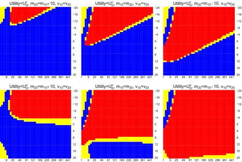
We repeat this process for different{m10,m20,v10,v20}and illustrate the optimal decisions on Figure 1. On each plot,
x-axis andy-axis correspond to the value ofv10andm10, blue and red indicate adding an arm and not adding an arm
are the optimal decision for a choice ofv10 andm10. The yellow region indicates 0 < |E(UDa|·) −E(UDNa|·)| < 0.01,
which could indicate indifference between the two decisions as the difference between the two expected utility is less than 0.01, orDNais better from monetary and logistics point of view. We include this region in the analysis to account for
the presence of Monte Carlo error when usingpmvnormonRto evaluate the probabilities. The first and the second row
1 9 25 49 81 121 169 225 289 361 441 20 16 12 8 4 0 −4 −8 −12 −16 −20 Utility=UDc, m
20=m10 10, v10=v20
1 9 25 49 81 121 169 225 289 361 441 20 16 12 8 4 0 −4 −8 −12 −16 −20 Utility=UDc, m
10=m20, v10=v20
1 9 25 49 81 121 169 225 289 361 441 20 16 12 8 4 0 −4 −8 −12 −16 −20 Utility=UDc, m
20=m10 10, v10=v20
1 9 25 49 81 121 169 225 289 361 441 20 16 12 8 4 0 −4 −8 −12 −16 −20 Utility=UDo, m
20=m10 10, v10=v20
1 9 25 49 81 121 169 225 289 361 441 20 16 12 8 4 0 −4 −8 −12 −16 −20 Utility=UDo, m
10=m20, v10=v20
1 9 25 49 81 121 169 225 289 361 441 20 16 12 8 4 0 −4 −8 −12 −16 −20 Utility=UDo, m
[image:8.595.49.549.351.685.2]20=m10 10, v10=v20
FIGURE 1 Optimal decisions: blue indicates adding an arm, red indicates do not add arm. The yellow region indicates 0<|E(UDa|·) −E(UDNa|·)|<0.01. First and second row correspond to usingU
c DandU
o
Din the framework,x-axis andy-axis correspond to the
of plots correspond to usingUDc andUDo, respectively, in the framework. Each column corresponds to the situation that
m10∕m20 < 1,m10∕m20 = 1, andm10∕m20 > 1.
We see that the choices of prior moments have some impact on the optimal decision. WhenUDc is considered in the decision-theoretic framework, choosing positive prior means and large prior variances would generally lead to adding an arm as the optimal decision. On the other hand, whenUDo is the objective of the study, it is better not to add the new treatment arm (whenm10 > m20), unless both the prior means and variances are very large. This analysis highlights the fact that it is more beneficial to add a new treatment arm to an on-going trial when the experimenters believe that the new treatment is considerably more efficacious than the control treatment and/or the initial treatment. Note that, when
m10 < <0,E(UDNa|X̄0.1 =5, ̄X1.1 = 8,nk2 = N2∕2)is very close to zero and henceDais the optimal decision on the top
left corner in the plots. In practise, consider prior means< < 0 for studies where positive magnitudes indicate that better treatment effect is not logical. This is because, if a treatment is believe to have negative treatment effect, it will not be chosen to be tested in a phase II or phase III clinical trial. We include this part in the illustration to remind users who might conduct such an analysis for studies that consider negative magnitudes as efficacious.
4
R E L AT I O N S H I P B ET W E E N STAG E O N E R E S P O N S E S A N D
O P T I M A L D EC I S I O N
We now explore how the optimal decision depends on the stage one data. Having chosen the utility and the values of
{m10,m20,v10,v20}, we can identify the optimal decisions for a range of stage one mean response of treatments. We assume
equal treatment randomisation probability for both stages, type one/family-wise error rate of 5%, and Bonferroni correc-tion when more than one experimental treatment is included in the trial. In what follows, we denote an optimal decision byD∗.
The first illustration considers an initial design that has one treatment arm and a control arm, whereas the second illus-tration has two treatment arms and a control arm. Without loss of generality, we depict the framework with a moderate and a large total sample size, respectively, in the examples.
4.1
Initial design: one treatment and a control arms
Consider a trial that has one treatment arm (k = 1) and a control arm (k = 0) initially, and stage-wise sample sizes
N1 = 400 andN2 = 300. After observing stage one responses wheren01 = n11 = 200, a decision must be made, to
either chooseDathat adds a new treatment arm (k = 2) to the concurrent trial, orDNathat do not add the new treatment
arm. FollowingDa, there will be three arms at stage two. Each arm will havenk2 = N2∕3 = 100, fork = 0,1,2 (two
treatments and a control). The family-wise error rate is controlled as two hypotheses will be tested at the end of the trial. We computeE(Uc
Da| X0̄ .1, ̄X1.1,nk2 = N2∕3)andE(U o
Da| X0̄ .1, ̄X1.1,nk2 = N2∕3)usingpmvnormonRas we did in
Section 3.2 but with different values ofx̄0.1, ̄x1.1and sample sizes. When the trial followsDNa, the two original arms will
haven02 = n12 = N2∕2 = 150, and the type one error rate is controlled for a treatment effect comparison between treatmentk = 1 and control treatmentk = 0. We can likewise computeE(UDNa| X̄k.1,k = 0,1,nk2 = N2∕2), and then
compare this value to the expected utility of adding an arm to identify the optimal decision for given values ofx0̄ .1, ̄x1.1.
In general, when the objective of a trial is to maximise the number of rejected hypotheses, we find that it is more beneficial to add a new treatment armk = 2 whenx1̄ .1−x0̄ .1is very large (indicating that treatmentk = 1 is considerably
better than the control treatment), or whenx̄1.1−x̄0.1is very small (indicating that treatmentk = 1 is considerably worse
than the control treatment). This could represent two extreme cases. (i) When we have enough power for testingH01, it is more beneficial to spend the remaining resources on testing the new treatmentk = 2. (ii) When we observe that the current treatment is not efficacious at all, we shall not spend all of the remaining resources on that treatment arm but open a new arm for studying another intervention in the on-going trial. On the other hand, for the trials that would consider a success when at least one hypothesis is rejected, the benefit of adding a new treatment arm to an on-going trial is substantial when the initial treatment is not effective. In the rare scenario where a promising finding is shown by stage one responses, adding a new treatment arm only results in negligible improvement to the utility of the trial. This is because the maximum ofUo
Dis one and rejecting one hypothesis with high probability is sufficient to declare a success.
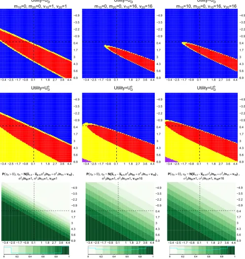
Figure 2 shows the optimal decisions for different pairs of mean response of treatments, wherex0̄.1is plotted on the x-axis, andx1̄.1on they-axis. Each column corresponds to using different values of{m10,m20,v10,v20}in the framework.
−3.4 −2.5 −1.7 −0.8 0.1 1 1.8 2.7 3.6 4.4 6.9 5.6 4.3 3 1.7 0.4 −0.9 −2.2 −3.5 −4.9
Utility=UDc
m10=0, m20=0, v10=1, v20=1
−3.4 −2.5 −1.7 −0.8 0.1 1 1.8 2.7 3.6 4.4 6.9 5.6 4.3 3 1.7 0.4 −0.9 −2.2 −3.5 −4.9
Utility=UDc
m10=0, m20=0, v10=16, v20=16
−3.4 −2.5 −1.7 −0.8 0.1 1 1.8 2.7 3.6 4.46.9 5.6 4.3 3 1.7 0.4 −0.9 −2.2 −3.5 −4.9
Utility=UDc
m10=10, m20=0, v10=16, v20=16
−3.4 −2.5 −1.7 −0.8 0.1 1 1.8 2.7 3.6 4.4 6.9 5.6 4.3 3 1.7 0.4 −0.9 −2.2 −3.5 −4.9
Utility=UDo
−3.4 −2.5 −1.7 −0.8 0.1 1 1.8 2.7 3.6 4.4 6.9 5.6 4.3 3 1.7 0.4 −0.9 −2.2 −3.5 −4.9
Utility=UDo
−3.4 −2.5 −1.7 −0.8 0.1 1 1.8 2.7 3.6 4.46.9 5.6 4.3 3 1.7 0.4 −0.9 −2.2 −3.5 −4.9
Utility=UDo
−3.4 −2.5 −1.7 −0.8 0.1 1 1.8 2.7 3.6 4.46.9 5.6 4.3 3 1.7 0.4 −0.9 −2.2 −3.5 −4.9
P 0, ~N(x x , /n /n v ) , /n =1, /n =1, v =1
−3.4 −2.5 −1.7 −0.8 0.1 1 1.8 2.7 3.6 4.46.9 5.6 4.3 3 1.7 0.4 −0.9 −2.2 −3.5 −4.9
P 0, ~N(x x , /n /n v ) , /n =1, /n =1, v =16
−3.4 −2.5 −1.7 −0.8 0.1 1 1.8 2.7 3.6 4.46.9 5.6 4.3 3 1.7 0.4 −0.9 −2.2 −3.5 −4.9
[image:10.595.49.547.53.579.2]P 0, N(x x , /n /n v ) , /n =1, /n =1, v =16
FIGURE 2 Optimal decisions whenUc
D(first row) andU o
D(second row) are considered in the framework. Last row shows the probabilities
thatx̄1.1−x̄0.1>0.x̄0.1is plotted onx-axis andx̄1.1ony-axis, dashed lines are plotted at approximately zero. Each column considers a choice
of{m10,m20,v10,v20}. Blue and red indicate adding an arm and not adding an arm are the optimal decision. Purple and yellow indicate that
both decisions have the same expected utility and 0<|E(UDa|·) −E(UDNa|·)|<0.01 [Colour figure can be viewed at wileyonlinelibrary.com]
same values ofx̄0.1and ofx̄1.1for different{m10,m20,v10,v20}in Figure 2. The interpretation of a plot on the first two rows
in Figure 2 is as follows. For a pair ofx0̄ .1 andx1̄ .1, the optimal decision is represented by a colour code: blue indicates Dahas a larger utility value given stage one data, red indicatesDNahas a larger utility value given stage one data. The
have the same expected utility. Both of this yellow and purple region could be interpreted as indifference between the two decisions as the gain is less than 0.01, orDNais better from monetary and logistics point of view.
The blue region on the second quadrant (top right) in all plots highlights thatDa is the optimal decision when the
initial treatment is not efficacious (as indicated by the light green region on the probability plots). We see that the region for whichDNais the optimal decision depend on the prior moments for𝜇k. Consider choosingUDc as the utility in the
decision-theoretic framework. As the prior variances,vk0increases, ie, when comparing (1,1) and (1,2) plots in Figure 2,
the red area (indicatesDNais the optimal decision) becomes smaller. This result is not surprising as the expected utility
gain of having two rejection of hypotheses is dominating, ie, givenZ(k,2), the relationship between variance parameters (that depend onvk0) and the last probability in (4) are monotonic increasing. Whenm10increases, ie, treatmentk = 1 is
believed to have a positive mean response, the red area is slightly enlarged and shifted to the left and upward when we compare (1,2) with (1,3) plots. This result is less intuitive and we conjecture that the larger sample size per treatment arm (of stage two) and the rejection boundary followingDNacontributes to the small increase in the area of the red region.
We find a similar pattern whenUo
Dis considered as the utility gain in the decision-theoretic framework. In addition to
that, there is a purple region where both decisionDaandDNagive the same utility value. Within these ranges ofx0̄ .1and ̄
x1.1, we only see the purple region in (2,2) and (2,3) plot in Figure 2. This occurs in the lower left quadrant (second row
of plots), where both the expected value ofUDo
Na and ofU o
Daare approximately equal to one, and the difference between
these values is trivial.
4.2
Initial design: two treatment and a control arm
We now illustrate the decision-theoretic framework for a two-stage trial that has two treatment arms,k = 1,2,and a control arm (k = 0) at stage one withnk1 = N1∕3 = 400, and stage-wise samplesN1 = 1200 andN2 = 1800. At the end
of stage one, we want to identify the best decision by considering the expected gains prior to implementation of stage two. With either decision, we control the family-wise error rate accordingly at 5%. The decision of not adding an arm would havenk2 = N2∕3 = 600 fork = 0,1,2. We can compute the expected utilities ofDNawith the probability as described in
Section 3.2 but conditioned onx̄k.1,k=0,1,2 and different sample sizes.
On the other hand, the decisionDawould involve adding in a third experimental arm, and thatnk2 = N2∕4 = 450,
fork = 0,1,2,3. To find the expected gain of adding a new treatment arm, we need to consider possible combinations of rejecting three hypotheses,H01,H02, andH03, which might be rejected at the end of the trial. In order words, for the trials that focus on maximising the number of rejected hypotheses, we evaluate
E (
Uc
Da|X̄k.1,k=0,1,2,nk2=N2∕4
)
=
3 ∑
v=1
v×P(reject exactlyvhypotheses out of three hypotheses);
for the other type of utility, we compute
E (
Uo
Da| X̄k.1,k=0,1,2,nk2=N2∕4
)
=
3 ∑
v=1
P(reject exactlyvhypotheses out of three hypotheses)
=1−P(not reject all three hypotheses),
which is equivalent to the disjunctive power when at least one of the rejected hypotheses is false under the null.
We can compute these probabilities usingpmvnormonR; with a bivariate normal distribution for the expected utility ofDNa, and a trivariate normal distribution for the expected utility ofDa. Note that the means and variances of both
multivariate normal distribution depend on the prior moments and stage one mean response of treatments. To be more specific, we have three mean response of treatments, ie,x̄0.1,x̄1.1, andx̄2.1, at the end of stage one of the trial. Given these
values and a choice of{m10,m20,m30,v10,v20,v30}, we can compute and compare the expected utility of each decision, with eitherUc
DorU o
Din the framework, to identify the optimal decision. We can repeat this procedure for differentx̄0.1,
̄
x1.1, andx2̄ .1for the investigation before seeing stage one of the trial.
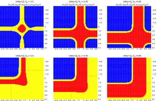
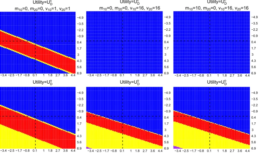
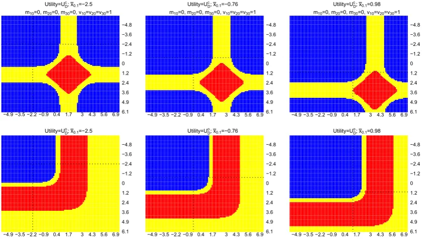
Figure 3 shows the results for this multiarm trial setting. Within each plot,x̄2.1is plotted on thex-axis andx̄1.1is plotted
on they-axis, dotted line corresponds to a value of the observedx0̄ .1. Each column corresponds to conditioning on a single ̄
x0.1; the first and second row of plots correspond to choosingUDc andUDo, respectively, in the framework. We see that there
−4.9 −3.5 −2.2 −0.9 0.4 1.7 3 4.3 5.6 6.9 6.1 4.9 3.6 2.4 1.2 0 −1.2 −2.4 −3.6 −4.8 Utility=U ; x =−2.5
m =0, m =0, m =0, v =v =v =1
−4.9 −3.5 −2.2 −0.9 0.4 1.7 3 4.3 5.6 6.9 6.1 4.9 3.6 2.4 1.2 0 −1.2 −2.4 −3.6 −4.8 Utility=U ; x =−0.76
m =0, m =0, m =0, v =v =v =1
−4.9 −3.5 −2.2 −0.9 0.4 1.7 3 4.3 5.6 6.9 6.1 4.9 3.6 2.4 1.2 0 −1.2 −2.4 −3.6 −4.8 Utility=U ; x =0.98
m =0, m =0, m =0, v =v =v =1
−4.9 −3.5 −2.2 −0.9 0.4 1.7 3 4.3 5.6 6.9 6.1 4.9 3.6 2.4 1.2 0 −1.2 −2.4 −3.6 −4.8 Utility=U ; x =−2.5
−4.9 −3.5 −2.2 −0.9 0.4 1.7 3 4.3 5.6 6.9 6.1 4.9 3.6 2.4 1.2 0 −1.2 −2.4 −3.6 −4.8 Utility=U ; x =−0.76
[image:12.595.48.552.46.371.2]−4.9 −3.5 −2.2 −0.9 0.4 1.7 3 4.3 5.6 6.9 6.1 4.9 3.6 2.4 1.2 0 −1.2 −2.4 −3.6 −4.8 Utility=U ; x =0.98
FIGURE 3 Optimal decisions whenUc
D(first row) andU o
D(second row) are considered in the framework.x̄2.1is plotted onx-axis andx̄1.1is
plotted ony-axis, dashed lines are plotted at approximately zero, and dotted lines correspond to the value of ax̄0.1. Each column considers a
value ofx̄0.1. Blue and red indicate that adding an arm and not adding an arm are the optimal decisions. Yellow indicates
0<|E(UDa|·) −E(UDNa|·)|<0.01 [Colour figure can be viewed at wileyonlinelibrary.com]
arm, and indifference between the decisions when 0<|E(UDa|·) −E(UDNa|·)|<0.01 (orDNais better from monetary and
logistics point of view).
The first quadrant (upper left quadrant that is divided by the dotted lines) on each plot corresponds to the situations that neither treatment k=1 nor treatment k=2 is better than the control treatment. The analysis shows that adding a new treatment k=3 to the existing trial is more beneficial than continuing the trial according to the initial design, when eitherUc
DorUDo is considered in the framework in this case.
When either (initial) treatment is better than the control arm (the second or the third quadrant), the framework with
Uc
D shows that the expected number of rejected hypotheses could be increased by adding a new treatment arm when
information for the initial arms is sufficient to claim the promising finding. On the other hand, the framework withUo D
would not add a new treatment arm in this case as the promising finding on any initial treatments would fulfil the trial objectives.
When both initial treatments are more efficacious than the control treatment, adding a new treatment arm could increase the expected number of rejected hypotheses provided that the initial treatments have sufficient information to claim the promising finding. This is reflected on the first row of plots, bottom right quadrant that is divided by the dotted lines. On the other hand, for a trial that focuses on declaring a success when at least one hypothesis is rejected, the bot-tom right quadrant in the second row of plots shows mainly red (DNais the optimal decision) and yellow (indifference or
DNais better from monetary and logistics point of view). This is because, if we have observed promising findings on both
initial treatment arms, the expected value ofUDo
Na is already close to one. Hence, the disjunctive power can no longer be
5
D I S C U S S I O N
The development of treatments for diseases is a long process. It is often the case that potential treatments are not available at the same time for conducting phase II/III studies. This work highlights the benefits of adding a new treatment arm to an existing study at an interim analysis. Instead of adding in a new treatment with certainty, we propose a decision-theoretic framework for studying when it is optimal to add an arm to an existing multiarm trial. We defined utility according to a design objective of a study, ie, (i) maximise the number of rejected hypotheses, and (ii) consider a success when at least one hypothesis is rejected. The expected value of these utilities is examples of expectation criteria and exceedance criteria, respectively. We consider a study design that initially hasKexperimental treatments and a control treatment. Having observed stage one of the trial, we identify the optimal decision by comparing the expected utility of using this initial design to the expected utility of using another design that hasK+2 arms at the second stage. Within the two-stage setting, we looked at the costs where adding in a new arm would reduce stage-two sample size per treatment arm and require adjustment to account for multiplicity. We acknowledge that multiplicity corrections might not be made in some multiarm trials. In this case, we only need to consider the cost of having smaller sample size per treatment arm and do the analysis of adding an arm analogously.
We presented how to investigate whether it is worth adding in a new treatment arm to an on-going multiarm trial based on the observed stage one mean response of treatments for a case study. We showed the impact of prior distributions on the optimal decisions. We also illustrated the analysis before the implementation of the trial. For the trial with more initial arms, the investigation can proceed analogously as described earlier. We find that, in a multiarm study, when none of the experimental treatments are more efficacious than the control treatment, adding in a new treatment arm to the on-going study is more beneficial than continuing the trial according to the initial design. This is because the newly added arm might demonstrate promising finding and hence increase the utility of the study. On the contrary, when the initial experimental treatments are considerably more efficacious than the control treatment, adding in a new treatment arm could potentially increase the expected number of rejected hypotheses. However, for multiarm studies that focus on disjunctive power, the decision to add a new treatment arm in this case is less substantial. This is because being able to claim any of the initial treatments as promising would have already fulfilled the study objective.
The aim of this manuscript is to present the notion of our decision-theoretic framework and the procedure of the investigation. We remind readers that the results of the illustrations presented in this paper are not comprehensive. For ease of exposition, we do not include the consideration of other aspects in the framework, eg, monetary cost of open-ing the new treatment arm. We also do not compare the utility of conductopen-ing a separate trial for the new arm when it was not added to the existing trial. Practitioners can formulate their utility and action spaces accordingly, as described in Section 2.3. Nevertheless, we have not considered choosingN2based on stage one observations in this work. A simple approach for optimisingN2at the same time could be specifying values for a cost per patient and reward for success.
Together with early stopping for futility and efficacy rules, future work could investigate how best to use the trial resources by constructing a different utility function. Without adding a prior distribution for the parameter of treatment effect, future work may also incorporate the probability of finding the treatment to be significant into the utility function. This could reflect that we are indirectly favouring treatments with higher effects without considering whether the null hypotheses are true or false.
We note that, as we consider a two-stage design whereby there is a possible change on total sample size per treatment arm, the type one error rate might be inflated. One could estimate the type one error rate, for example, by consider-ing a null distribution for the responses and assume a prior distribution for the decision markconsider-ing, then approximate the type one error. This investigation could show the magnitude of the inflation, and the experimenters could con-sider the significance of this inflation when making the decision for implementation. Alternatively, we could avoid this issue by replacing the aforementioned inference procedure with a combination test19and conduct the investigation on
adding arm adaptation in a similar fashion. Future work could consider using a recursive combination test20or a group
sequential approach to adjust the final test21,22in a decision-theoretic framework for trials that have multiarm multistage
settings.
that initially has two arms and which aims to maximise the number of rejected hypotheses,UDc, are exceptional cases. For these cases, ie, when prior means≥0 and prior variances are large (correspond to (1,2) and (1,3) plots in Figure B1), we find that adding the new treatment arm is the optimal decision given those observed stage one mean responses. This finding is not surprising as the initial trial resources are not affected by the decision and adding in the new arm increases the chance of rejecting an extra hypothesis.
Here, we have focused on a normal outcome. To our knowledge, many clinical trials in psychiatry and psychology stud-ies involve normally distributed outcomes. The systematic review by Wason et al23considered 59 multiarm trials, of which
22 (37%) have continuous primary outcome. We think it is possible to amend such a decision-theoretic framework for trials with a binary outcome. This can be done by changing the test statistics and making some assumptions about the variances of the response probabilities. For other types of outcome, the framework can be applied when the trial sample sizes are large. This is because the test statistics can be approximated by the normal distribution even if the individual out-come data is not normal. We acknowledge that most of the trials in practise have several secondary outout-comes that it may be important to consider, or involve subgroup analysis and follow-up measurements. Further investigation is required to account for these. Besides that, we have not facilitated the standard power and sample size calculation in the framework. Wason et al24investigated sample size for a multiarm multistage drop-the-losers design. Future work could consider the
impact of adding an arm on this design, different approaches and perspectives for the sample size calculation,25-32and also
account for the presence of missing responses. Some authors33,34have tackled the presence of missing responses from the
perspective of design of experiments, by having more subjects enrolled to the arm that is expected to have higher miss-ing response rate. Other future work could incorporate stage one control responses when makmiss-ing pair-wise comparison between the newly added treatment and the control treatment. A caveat on this aspect is that there might be population drift if the overall duration of a trial is long. One could also consider the impact of using different randomisation strate-gies such as a response adaptive randomisation procedure that is robust to time trend.35We note that we have not focused
on parameter estimation in this work. In seamless phase II/III clinical trials with early stopping for futility, methods have been proposed for unbiased estimation.36-38Stallard and Kimani39indicated that (conditionally) unbiased estimators for
the trial that adds arm(s) could be complicated to derive. This highlights the fact that more research on adding arm(s) to an on-going trial is required.
AC K N OW L E D G E M E N T S
This research has been funded by the Medical Research Council (grant codes MR/N028171/1 and MC_UP_1302/4). We acknowledge Dr. Siew Wan Hee for comments on this work. Data sharing is not applicable to this article as no new data were created or analyzed in this study.
O RC I D
Kim May Lee https://orcid.org/0000-0002-0553-973X
R E F E R E N C E S
1. Sydes MR, Parmar MK, Mason MD, et al. Flexible trial design in practice - stopping arms for lack-of-benefit and adding research arms mid-trial in STAMPEDE: a multi-arm multi-stage randomized controlled trial.Trials. 2012;13(1):168.
2. Park JW, Liu MC, Yee D, et al. Adaptive randomization of neratinib in early breast cancer.N Engl J Med. 2016;375(1):11-22.
3. Alexander BM, Ba S, Berger MS, et al. Adaptive global innovative learning environment for glioblastoma: GBM AGILE.Clin Cancer Res. 2018;24(4):737-743.
4. Cohen DR, Todd S, Gregory WM, Brown JM. Adding a treatment arm to an ongoing clinical trial: a review of methodology and practice.
Trials. 2015;16(1):179.
5. Elm JJ, Palesch YY, Koch GG, Hinson V, Ravina B, Zhao W. Flexible analytical methods for adding a treatment arm mid-study to an ongoing clinical trial.J Biopharm Stat. 2012;22(4):758-772.
6. Ventz S, Alexander BM, Parmigiani G, Gelber RD, Trippa L. Designing clinical trials that accept new arms: an example in metastatic breast cancer.J Clin Oncol. 2017;35(27):3160-3168.
7. Ventz S, Cellamare M, Parmigiani G, Trippa L. Adding experimental arms to platform clinical trials: randomization procedures and interim analyses.Biostatistics. 2018;19(2):199-215.
9. Yuan Y, Guo B, Munsell M, Lu K, Jazaeri A. MIDAS: a practical Bayesian design for platform trials with molecularly targeted agents.
Statist Med. 2016;35(22):3892-3906.
10. Hobbs BP, Chen N, Lee JJ. Controlled multi-arm platform design using predictive probability.Stat Methods Med Res. 2018;27(1):65-78. 11. Raïffa H, Schlaifer R.Applied Statistical Decision Theory. Cambridge, MA: MIT Press; 1961.
12. DeGroot MH.Optimal Statistical Decisions. Hoboken, NJ: Wiley; 1970.
13. Smith JQ.Decision Analysis: A Bayesian Approach. Boca Raton, FL: Chapman and Hall; 1988.
14. Hee SW, Hamborg T, Day S, et al. Decision-theoretic designs for small trials and pilot studies: a review.Stat Methods Med Res. 2015;25(3):1022-1038.
15. Berry DA, Ho C-H. One-sided sequential stopping boundaries for clinical trials: a decision-theoretic approach. Biometrics. 1988;44(1):219-227.
16. Dmitrienko A, Paux G, Brechenmacher T. Power calculations in clinical trials with complex clinical objectives.J Jpn Soc Comput Stat. 2015;28(1):15-50.
17. Radnovich R, Scott D, Patel AT, et al. Cryoneurolysis to treat the pain and symptoms of knee osteoarthritis: a multicenter, randomized, double-blind, sham-controlled trial.Osteoarthr Cartil. 2017;25(8):1247-1256.
18. Lee PM.Bayesian Statistics: An Introduction. London, UK: Arnold; 2004.
19. Bauer P, Köhne K. Evaluation of experiments with adaptive interim analyses.Biometrics. 1994;50(4):1029-1041. 20. Brannath W, Posch M, Bauer P. Recursive combination tests.J Am Stat Assoc. 2002;97(457):236-244.
21. Stallard N, Todd S. Sequential designs for phase III clinical trials incorporating treatment selection.Statist Med. 2003;22(5):689-703. 22. Stallard N, Friede T. A group-sequential design for clinical trials with treatment selection.Statist Med. 2008;27(29):6209-6227.
23. Wason JMS, Stecher L, Mander AP. Correcting for multiple-testing in multi-arm trials: is it necessary and is it done?Trials. 2014;15(1):364. 24. Wason J, Stallard N, Bowden J, Jennison C. A multi-stage drop-the-losers design for multi-arm clinical trials.Stat Methods Med Res.
2017;26(1):508-524.
25. Stallard N, Posch M, Friede T, Koenig F, Brannath W. Optimal choice of the number of treatments to be included in a clinical trial.Statist Med. 2009;28(9):1321-1338.
26. Wason JMS, Mander AP, Thompson SG. Optimal multistage designs for randomised clinical trials with continuous outcomes.Statist Med. 2012;31(4):301-312.
27. Stallard N. Optimal sample sizes for phase II clinical trials and pilot studies.Stat Med. 2012;31(11-12):1031-1042.
28. Bowden J, Wason J. Identifying combined design and analysis procedures in two-stage trials with a binary end point.Statist Med. 2012;31(29):3874-3884.
29. Wason JMS, Jaki T. Optimal design of multi-arm multi-stage trials.Statist Med. 2012;31(30):4269-4279.
30. Mander AP, Wason JMS, Sweeting MJ, Thompson SG. Admissible two-stage designs for phase II cancer clinical trials that incorporate the expected sample size under the alternative hypothesis.Pharmaceutical Statistics. 2012;11(2):91-96.
31. Wason JMS, Mander AP. Minimizing the maximum expected sample size in two-stage phase II clinical trials with continuous outcomes.
J Biopharm Stat. 2012;22(4):836-852.
32. Stallard N, Miller F, Day S, et al. Determination of the optimal sample size for a clinical trial accounting for the population size.Biometrical Journal. 2017;59(4):609-625.
33. Lee KM, Biedermann S, Mitra R. Optimal design for experiments with possibly incomplete observations. Statistica Sinica. 2018;28:1611-1632.
34. Lee K, Mitra R, Biedermann S. Optimal design when outcome values are not missing at random.Statistica Sinica. 2018;28(4):1821-1838. 35. Villar SS, Bowden J, Wason J. Response-adaptive designs for binary responses: how to offer patient benefit while being robust to time
trends?Pharmaceutical Statistics. 2018;17(2):182-197.
36. Stallard N, Todd S. Point estimates and confidence regions for sequential trials involving selection. J Stat Plan Inference. 2005;135(2):402-419.
37. Kimani PK, Todd S, Stallard N. Conditionally unbiased estimation in phase II/III clinical trials with early stopping for futility.Statist Med. 2013;32(17):2893-2910.
38. Kimani PK, Todd S, Stallard N. A comparison of methods for constructing confidence intervals after phase II/III clinical trials.Biometrical Journal. 2014;56(1):107-128.
39. Stallard N, Kimani PK. Uniformly minimum variance conditionally unbiased estimation in multi-arm multi-stage clinical trials.
Biometrika. 2018;105(2):495-501.