Autonomous real time object detection and identification

(1)

Autonomous Real-time Object Detection

and Identification

Gruffydd Morris

Supervisors:

Professor Plamen Angelov

Dr Graham Lovegrove

Dr Graeme Knight

School of Computing and Communications

Lancaster University

Thesis for the degree of

Doctor of Philosophy

(2)

(3)

Declaration

I hereby declare that except where specific reference is made to the work of others, the contents of this thesis are original and have not been submitted in whole or in part for consideration for any other degree or qualification in this, or any other university. This thesis is my own work and contains nothing which is the outcome of work done in collaboration with others, except as specified in the text and Acknowledgements.

(4)

iv

Live as if your were to die tomorrow. Learn as if you were to live forever. Mahatma Ghandi

I believe that failure comes from giving up. If you never choose to fail, if you never choose to give up, then you’re just in the process of making it happen.

(5)

Acknowledgements

(6)

Abstract

(7)

List of figures

1.1 The process of data analysis . . . 3

1.2 An example frame from which operators need to detect this small target . . 5

1.3 The progress of computing measured in cost per million standardized opera-tions per second (MSOPS) deflated by the consumer price index [104] . . . 8

2.1 One-dimensional edge profiles. [58] . . . 18

2.2 Roberts Operator. [58] . . . 19

2.3 Sobel Operator. [58] . . . 20

2.4 A comparison of Edge Detectors. a) Original image b) Filtered image, c) Simple gradient using 1 x x2 and 2 x 1 masks, d) Gradient using 2 x 2 masks, e) Robert cross operator, f) Sobel operator, g) Prewitt operator [58] . . . 21

2.5 Laplacian Operator, derived as the second order differential [58] . . . 22

3.1 Simple rotating rectangles . . . 44

3.2 Vehicle accident scene . . . 45

3.3 Busy people scene . . . 45

3.4 Z-axis perspective occlusion . . . 46

3.5 A comparison of RDE and Greyscale applied to rotating rectangles . . . 46

3.6 A comparison of RDE and Greyscale applied to a traffic accident . . . 47

3.7 A comparison of RDE and Greyscale applied to a busy walkway . . . 47

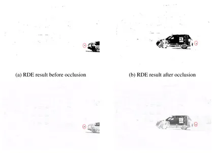
3.8 A comparison of RDE and Greyscale results before and after an occlusion event. The red circle indicates the detection of the person with a white jersey walking down the path, see figure 3.4 . . . 48

3.9 Windowed density estimation applied to the two counter-rotating rectangles 52 3.10 Windowed density estimation applied to the busy walkway. . . 52

3.11 Windowed density estimation applied to the road traffic accident scene. . . 52

(13)

List of figures xiii

3.13 Helicopter chase scene with a motorbike and car . . . 59

3.14 Panning motion of a street scene . . . 60

3.15 Different key point detection algorithms used for motion estimation on the Helicopter and Panning videos . . . 61

3.16 Different key point detection algorithms used for motion estimation on the Z-axis video . . . 62

3.17 Key point matching algorithms used for motion estimation on the Helicopter and Panning videos . . . 63

3.18 Filtering algorithms used for motion estimation on the Helicopter and Pan-ning videos . . . 64

3.19 Interpolation algorithms used for motion estimation on the Helicopter and Panning videos . . . 65

3.20 Computer Vision hierarchical model . . . 69

3.21 OSI network model . . . 69

3.22 Typical operating system kernel hierarchy . . . 69

3.23 Example hierarchy for game design . . . 70

3.24 V-Model for software development . . . 71

3.25 AGILE model for software development . . . 71

3.26 A cyclic framework proposed for computer vision . . . 72

4.1 Edge flow components, and in green, the output at each component stage . . 76

4.2 Greyscale RDE applied to moving camera to define object texture edges . . 77

4.3 WIDE applied to moving camera to define object texture edges . . . 77

4.4 X and Y Sobel filters . . . 78

4.5 Left, gradient values assigned for an x-plane Sobel filter. Right, gradient values assigned based on a y-plane Sobel filter . . . 78

4.6 Result of a Sobel filter in the y-plane applied to RDE image. The gradient values have been coloured for a better visual effect – blue indicates large gradient changes, whilst green is a smaller gradient value. Yellow indicates areas of no edge gradients (and therefore no edges – the texture of an object). 79 4.7 Pixels linked in an edge, and the area of influence of the edge. . . 81

4.8 (a) Contiguous clustering of gradients from Sobel stage (b) Result of optical flow applied to clusters . . . 82

(14)

List of figures xiv

4.10 Motion estimation result from scene (left) Edge flow result from scene (right). Red boxes are included on edge flow to highlight detections more clearly. 640 x 360 pixels . . . 85 4.11 A comparison of Edge Flow with Motion Estimation and Optical Flow on

the Helicopter video . . . 85 4.12 Second test video, dashboard mounted camera . . . 86 4.13 A comparison of Edge Flow with Motion Estimation and Optical Flow on

the dashboard video . . . 86 4.14 Video 3 scene - drone flying with multiple axis of motion . . . 88 4.15 A comparison of Edge Flow with Motion Estimation and Optical Flow on

the UAV video . . . 88 4.16 Conceptual framework for human object detection, [18] . . . 92 4.17 WISE components, and in green, the output at each component stage . . . . 95 4.18 An illustration on how the edge influence (and thus membership) propagates

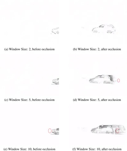
across the image . . . 96 4.19 This set of images shows the results of the WISE technique when applied

with different window sizes. (a) is with window size 2, (b) is a window size of 3, and (c) is a window size of 4. The Sobel filter has a consistent size of 7x7 for each image . . . 98 4.20 This set of images shows the results from changing the size of Sobel filter

from 3x3 (a), 5x5 (b) and 7x7 (c) with the WiDE window size set to 3. . . . 98 4.21 Here is a range of visualisations for the clustering results of WISE. The

first (a) is a view of the clustering, using a bounding rectangle to include the pixels that represent and individual texture. The bounding box image is included to highlight the extent of each cluster and reinforce that the clusters are separate distinguishable textures. Both the (b), and (c) images show the actual pixels of a cluster represented with a colour overlay. . . 100 4.22 Clustering results for WISE applied to the busy road intersection scene,

introducing a greater 3D differential for the algorithm to handle. Figure (a) shows the rectangular cluster representation. Figures (b) and (c) show the clusters pixel-wise using a colour overlay. One is just the cluster pixels (b), and the other is the cluster pixels overlayed onto the original image (c) . . . 100 4.23 Edge detection results for WISE (a), Edge Flow (b) and Canny Edge Detector

(15)

List of figures xv

4.24 Edge detection results for WISE (a), Edge Flow (b) and Canny Edge Detector (c) applied to the busy road intersection scene, introducing a greater 3D

differential for the algorithms to handle . . . 101

4.25 These images show the comparison of Grab Cut (a), Mean Shift (b), and WISE (c) on the helicopter scene . . . 102

4.26 These images show the comparison of Grab Cut (a), Mean Shift (b), and WISE (c) on the helicopter scene . . . 102

4.27 WISE applied to the helicopter scene. . . 104

4.28 WISE applied to the dashboard scene. . . 104

4.29 WISE applied to the UAV scene. . . 104

4.30 WISE components with optical flow addition . . . 108

4.31 WISE and Optical Flow applied to the helicopter video . . . 108

4.32 WISE and Optical Flow applied to the dashboard video . . . 109

4.33 WISE and Optical Flow applied to the UAV video . . . 109

4.34 Additional frame with greater UAV motion . . . 110

5.1 (a) Original Image (b) Fuzzy Edge Detector [65] (c) ACO edge detector [79] (d) Neural Network edge detector [13] (e) Genetic Algorithm edge detector [17] (f) Universal Gravity edge detector [139]. Images obtained from [1] . . 113

5.2 (a) WIDE with window 2, (b) WIDE with window 3, (c) WIDE with window 4, (d) WIDE with window 5 . . . 114

5.3 Edge detection results from [33] for fast edge detection using structured forests115 5.4 (a) WIDE on people with window of 4, (b) WIDE on barn picture with window of 4, (c) WIDE with window of 6 on coyote picture . . . 115

5.5 A selection of varying Image Segmentation techniques applied to the BSD database. (a) Ultrametric Contour Map [10], (b) Edison and IHS Image Segmentation methods [158], (c) Bottom Up Aggregation [3], SWA V1 [46], Normalised cuts [84], Mean-shift [27] . . . 119

5.6 WISE applied to the images used by other techniques. The leftmost image is the actual pixels of the detected texture patches overlaid on the original image. The rightmost image is the individual texture patch boundaries. (a) and (b) Giraffe, (c) and (d) Woman with a baby, (e) and (f) Surfer . . . 120

(16)

List of figures xvi

5.8 Results from different object detection by classifiers methods, applied to the YouTub-Objects database [113]. (a) Hough Forest Object Detection [45], (b) Fast object segmentation [109] . . . 124 5.9 WISE applied to the datasets used by the methods presented above. The

leftmost image is the actual pixels of the detected texture patches overlaid on the original image. The rightmost image is the individual texture patch boundaries. . . 125

6.1 WISE objects detected, with optical flow and object boundaries . . . 130 6.2 Clustering of the optical flow results using CEDAS. The x-axis shows angle

of motion (−π toπ), and y-axis shows magnitude of motion, normalised

between 0 and 1. . . 131 6.3 A series of consecutive frame analysis results from CEDAS, applied to the

scene with the person running in circles . . . 132 6.4 Helicopter police chase video . . . 136 6.5 UAV flight video . . . 136 6.6 Clustering of objects in the helicopter video, resulting in the characterisation

of different object types. . . 137 6.7 Clustering of objects in the UAV video based on motion features . . . 137

(17)

List of tables

4.1 Characteristics of some sample novelty detection algorithms . . . 83

4.2 Detection performance for video 1 . . . 85

4.5 Performance analysis of each algorithm across each test video stream . . . 89

5.1 The performance of different edge detection techniques on the BSD500 [10] data set obtained from [33] and compared with the WIDE technique over 3 different window sizes . . . 116

5.2 The performance of different image segmentation techniques on the BSD500 [10] data set obtained from [10] and compared with the WISE technique over 3 different window sizes . . . 122

5.3 Comparison of the results presented by [45] with WISE over 3 different window sizes . . . 126

(18)

Glossary

Term Description

Candidate objects Candidate objects are texture patches that represent objects of interest.

CEDAS Online clustering process defined in [57]

Computer Vision The field is interdisciplinary that deals with how computers or artificial devices can gain a high level of understanding from images or video streams

Edge clustering The same process as edge linking, the terms may be used interchangeably.

Edge linking The process of joining contiguous edge pixels together to form texture patches

F-measure Measures the average squared colour error of the segments, penalizing over-segmentation by weighting proportional to the square root of the number of segments. It requires no user-defined parameters and is independent of the contents and type of image.

Texture patch Used to describe the area of textured pixels linked together by the edge linking of WISE. They form candidate objects Unmanned Aerial Vehicle (UAV) An unmanned aircraft that is typically used by the military

and border protection services to gain advanced

reconnaissance. They usually have on-board cameras, and limited computational processing power.

(19)

Chapter 1 Introduction

This chapter introduces the scope of the research undertaken in this thesis. Firstly it considers the wider field of data analysis and data gathering through the use of optical devices, and then considers application specific problems. How computer vision as a whole is employed in a variety of ways to tackle these problems is introduced followed by scoping the particular problem area of this research and the questions associated with it. The scope of the work is condensed into the specific research conducted throughout the remainder of the thesis. Chapter 2 specifically deals with the research papers relevant to the field of research, and how existing research can contribute to resolving the questions proposed here.

1.1 Scope

(20)

[image:20.595.141.471.107.253.2]

1.1 Scope 3

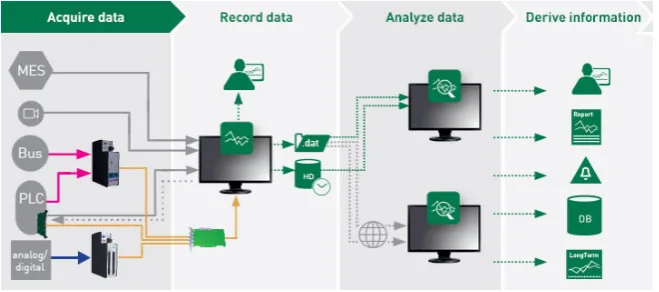
Fig. 1.1 The process of data analysis

(21)

1.2 Motivation 4

1.2 Motivation

In a world where sensors for data acquisition are used on an ever expanding scale, there is a requirement to efficiently process and interpret the data into meaningful information. There are millions of cameras; in the UK alone there are an estimated 5.9 million surveillance cameras in operation [142]. A much greater number of optical cameras are included on mobile phones, and are now estimated to outnumber the human population on the earth [20]. Additionally, cameras are gathering data from vehicles (such as aircraft, border patrol teams, satellites, unmanned aerial and ground vehicles, and amateur video recordings). The total volume of data gathered by these devices is astronomical, and far outweighs the time available to humans to review all of the gathered data. This all contributes to the mass volumes of video data being recorded and stored, some with useful information or important observations that, at present, require human observers to extract them. Considering just the CCTV context of the UK, over 141 million hours of video is recorded every day. That means everyone in the population would have to watch 2.2 hours of surveillance video each day to get through the entire recorded data. The number of hours each person would have to watch to cover all the gathered CCTV data is large and impractical. There are, in reality, many less operators to view all this information and many will need to review several cameras at once to try to identify problems, issues and incidents [63]. This is without taking into account the human factors such as attention span and sleep requirements of an operator [133]. The automation of surveillance camera systems would go a long way to ensuring that security requirements are met, such that useful information or important observations are not missed; as well as to reduce the load and pressure on operators. To this end, there is the goal of enabling computers to interpret visual data from these optical devices and process the data in a meaningful way to produce useful information as its outputs. The field of research into this technology is collectively known as computer vision.

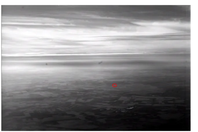
Cameras are regularly used as sensors on unmanned aerial vehicles (UAVs) as recon-naissance and intelligence gathering systems [49] [103] and used for support of front line troops on operations [31]. The cameras on these vehicles can be of the order of 1 – 2 gigapixels with frame rates of the order of 25 -100 frames per second, meaning the data is gathered at terapixels per second, that is 3 -5 terabytes of information per second [9]. As this reconnaissance data is gathered, operators on the ground have to sift through each frame looking for important objects or points of interest to support the operations [31]. Figure 1.2 shows an example of a frame from a UAV, and the small object of interest that each operator is expected to see.

(22)

[image:22.595.139.481.99.327.2]

1.3 Computer Vision Goals and Human Replication 5

Fig. 1.2 An example frame from which operators need to detect this small target

that promotes algorithm efficiency. The potential application is however not limited to the UAV environment, and would be suitable to any sensor application that would require detection and tracking of features of interest. The outline of the research is to:

Returning to the UAV application, using the cameras on board the UAV, :

• Develop systems to automatically detect and track dynamic objects or features of interest in a real time live video stream environment. The development would be highly computationally and memory efficient, lending itself to being used on platforms with limited computing power such as UAVs.

• Combine these highly computational efficient online, real-time information extraction algorithms with capable self-learning algorithms that can detect and track objects in a live sensor environment with dynamically changing scenery.

1.3 Computer Vision Goals and Human Replication

(23)

1.3 Computer Vision Goals and Human Replication 6

and signal transfer to the output display. Software in the modern era is sufficiently advanced to enable computers to take a set of inputs, process them and provide a set of intelligent results that gives the impression of autonomous behaviour. Research into computer vision has allowed computers to take or receive a visual input as stimuli (data), conduct some processing (compute) and provide intelligent results on its output (information). The visual stimuli for the purposes of this work are data from colour cameras; and is referred to as simply a camera from herein. The generated image from this camera is made up of red, green and blue picture elements (RGB pixels).

(24)

1.4 Real-time algorithms 7

of a vision system, and other techniques bring together many components to achieve an all round detection and identification system.

1.4 Real-time algorithms

In this research there is a consistent reference to real-time processing or real-time analysis. Real-time systems provide a constraint on the computer system in which the data must be analysed and the results outputted. This is also known as computational deadlines [108]. Being correct and real-time does not mean just outputting a correct calculation, it is also dependent on being within the time constraint [130]. The time constraint can be hard (safety critical systems for example), whereby missing any time deadlines constitutes a system failure, firm (network packets for example) where by missing some time deadlines are tolerable but the service or operational speed of the system may be degraded. The work packet is useless if the time deadline is missed (e.g. retransmission of network packet if arrival deadline is missed). Finally there are soft real-time systems, whereby the performance is degraded if the time deadline is missed, and the usefulness of the work packet is degraded if the time deadline is missed - e.g. system fault and condition data. It is important to identify that brute force processing does not necessarily yield a real-time system [136]. A computer may have high data and processing throughput (such as a Cray supercomputer [123]), however the results may still not be provided for several minutes (complex protein folding for example [147]). Conversely a low power system, with limited processing capacity may be considered as real-time, despite its limited capacity, if the result of the system is returned in sufficient time to immediately affect its environment e.g. temperature regulation of a green house -the windows and heaters are controlled in real-time to regulate -the internal temperature of the green house. Referring back to the brute force type processing, the computing power industry is consistently following Moore’s Law, and in some cases exceeding it [93]. In the graphic shown in figure 1.3, the cost per GFLOP [104] is decreasing at rapid rate, and is expected to continue in the immediate future. There is therefore scope for using parallelism on existing computer vision algorithms (such as optical flow, or image segmentation) using the brute force of this computational power to make them operate in real-time, [110]. There are some drawbacks to this approach.

(25)

[image:25.595.117.481.246.560.2]

(26)

• If the image resolution is sufficiently large, even with the huge processing capabilities, real-time capability will eventually be reduced or unattainable.

• Not all application areas will be able to utilise the high powered processing due to other system or environmental constraints (e.g. the power capacity of a UAV is limited, thus the processing power available will also be limited).

• Despite the cost per GFLOP reducing, using a brute force approach does not address the requirement of cost outlay for high powered computing systems that would be required to make some algorithms real-time capable

• The complexity of some algorithms are such that not all aspects are necessarily suitable for parallelism. Thus the gains are not necessarily directly proportional to the increase in processing power.

It is important to note that real-time is often confused with an on-line system, or at least the terminology is used independently. Whilst they are similar, and both relate to the time of the processing, they are also distinctly different. Online or offline processing refers to when the system begins processing the data. An online system is continuously processing data as it arrives into the system, and does not wait for a collection or data set to be gathered before processing the available data. Conversely an offline system waits for the entire dataset to be gathered, and then subsequently processes the data. An offline system can be real-time, provided that it yields the results of the processing in a timely manner after the data has begun being processed / analysed. Equally an on-line system does not have to be real-time, whilst the data processing is continuous and begins as soon as a data sample is received, the result may not have to be returned with some time constraint. An example of a system that is on-line yet not real time is the SETI program, whereby the data samples are processed as they are received from the Archiebo telescope, yet the results of the analysis of the particular data set are not outputted for several hours [99].

(27)

1.5 Autonomy or Intelligence 10

1.5 Autonomy or Intelligence

Humans could be considered either a very lazy species, or one that likes to optimise tasks such that other tasks can be accomplished simultaneously. There are clear examples of both in the technological world that we live in [44]. To that end, many of the electronic systems that we see in daily life can be considered, to a degree, autonomous. That is, the machines are given a task to do, and they will conduct the processing required until the task is complete and provide and output, without any intermediate intervention. If you consider the use of a washing machine, the user puts in clothes and the washing powder, selects a cycle, and presses go. This could be considered an initialisation of the autonomous system. During the wash cycle, provided no error occurs, the machine will autonomously (i.e by itself) wash the clothes and discard the dirty water. However, the automation is limited such that it cannot compensate for unknown or unforeseen scenarios [138] [11]. To address these scenarios, input from the user is required. Intelligent systems address this by having a flexible interpretation of the input and have ability to handle unexpected or unknown scenarios, autonomously without necessarily having human intervention [42]. Some of these can be supervised systems, such that there is an intelligent agent yet operators feed in additional information or parameters to support the decision making process [124]. Other, fully unsupervised techniques, do not require the input of parameters or intervention by users to learn about new and unknown scenarios [115]. The intelligence is often referred to as machine learning, whereby the system is interpreting its environment and creating new rules or constraints for autonomous operation based on different and changing inputs.

(28)

Chapter 2 Computer Vision and Existing Research

Computer Vision has grown exponentially over the last 30 years such that it is a large research field, with many approaches that are derived to solve a wide range of vision problems. Latterly, the human objective to employ autonomous agents such as driver-less cars and unmanned surveillance vehicles has fuelled more research and funding into the field of computer vision. This chapter looks through the wealth of computer vision techniques available and what benefits and drawbacks some of the techniques have.

2.1 The Field of Computer Vision

The field itself can broadly be broken down into a number of sub categories, each of which have their own objectives in terms of data analysis and output. That is:

• Image Enhancement - image denoising, brighness and Gamma corrections, histogram analysis

• Transformations - Homography, Affine transforms, Warping, Data space manipulation

• Filtering, Fourier transforms and Image Compression - Image analysis, optimisation and size reduction (compression)

• Colour Vision - Colour mapping, colour management, colour profile analysis

• Feature extraction - Edge Detection, Corner Detection, Key-point Detection

• Pose Estimation - visual geometry, orientation and angle estimation, projections and modelling

(29)

2.1 The Field of Computer Vision 12

• Visual Recognition - feature transforms (SURF, SIFT), object recognition, posture and gesture recognition, facial and finger print recognition

The sub-categories fit three main criteria of image and video processing:

• Image manipulation.In this criteria, the processing is focussed on filtering, denoising and optimising the image itself without any notion of "what" is in the image. The processing may augment or highlight certain objects, and de-emphasis others, but this is mainly a process where the augmentation and de-emphasis are tuned based on the objects the user wants to see more or less of. The categories that fit into this criteria are Image Enhancement, Filtering, and Colour Vision although there may be some crossover from Registration and Transformations

• Detection. This criteria primarily focussed on detecting features, key-points and candidate objects in the image. The detection phase is an essential part of image understanding such that computer systems can understand and interpret a scene. In some cases detection can be pixel feature extraction [50] [75] and detection of contours and edges [33] [23]. It can also be in the form of detecting important points in the image such as keypoint detection [78] [14] [2] and optical flow detection [81] [55] [157] [149] or detecting the pixels potential associated together (candidate objects) such as background subtraction [137] [37] [4]. The categories that fit this criteria are Feature Extraction, Registration, and Visual Recognition

• Image Understanding. Technically, this criterion could not exist without the existence of one or both of the previous criteria. It is to do with interpreting and analysing the image such that situational and environmental understanding of the scene or image can be achieved. The understanding can be achieved following some image manipulation; for example if the result of the manipulation yields two distinct image colours, a level of understanding (provided appropriate rules are present) of the image can be achieved. Similarly if there are a series of candidate objects present from the detection phase, an understanding of these objects can be achieved through further processing. Categories in this criteria are pose recognition, visual recognition and transformations. Whilst the latter two are also applicable to the previous criterion, aspects of them are directly applicable here (such as facial recognition; the keypoint detection extracts the appropriate detections, and then this phase applies the matching analysis to a database or reference image)

(30)

1. Novelty detection in a moving image plane

2. Object identification

3. Behaviour analysis – anomaly detection, trajectory analysis

4. Tracking of one or more detected objects in the image frame

5. Collaborative (swarm) of UAVs working together to achieve a common goal

6. Exploration of parallelisation in software agents

Each aspect contains different types of research, and over the next paragraphs the details of each area are explored.

2.1.1 Novelty Detection

Novelty detection is the first phase of computer vision image processing. The principle is to detect a foreground novelty from the clutter of the background. One of the most commonly used methods is background subtraction using KDE (Kernel Density Estimation). This relies on generating a statistical model of the background of an image that is representative and discriminates from new foreground novelties in the image [37]. The complexity required increases markedly when the background itself is not constant (as it would be with a moving camera). Here, two distinct problems exist and define the direction of the research:

1) The offline computational requirement of KDE is not suitable for UAV applications; the requirement is to have an online, real-time processing of the image data.

2) With the background no longer a constant, subtraction of the background using the traditional KDE will result in high noise, potentially leading to false detections.

(31)

These approaches, however, assume the objects are to be initialised manually. Research into merging or combining both recursive background subtraction and SIFT / SURF approaches is a possible progression which could yield a highly discriminatory novelty detection capability in a dynamic video stream which is both robust and computationally efficient [78] [14]. One particular development area of interest is to detect novelties in terms of a new patch / object even if it is not moving. For example, comparing with a previous days images and identifying that this new patch / object was not there previously (examples of such could be mobile SAM sites, military camp, hostages etc.).

2.1.2 Object Identification

Whilst detection of novelties in an image frame is an important first stage in image analysis, there is nothing at this stage to identify whether this is an object of interest or not – one could say that the information itself has not yet been extracted, just “potential” information areas. To identify foreground objects, some sort of clustering and/or classifier or labeller is needed to clearly distinguish objects. A common approach to identifying key areas is image segmentation using clustering and/or classification of the feature space. Image segmentation is a method to partition the feature space by labelling pixels that share similar visual features or properties, and connecting the pixels with the same labels in some meaningful way [102]. There are approaches such as region growing, watershed, clustering and fuzzy set techniques, which are either for a specific domain or image field, and require significant offline processing to work. In the work of Othman et al [107] it is proposed that an Evolving Fuzzy Inference System is used to classify objects within a static MRI. This approach is based on the eClass semi-supervised classifier [4]. An alternative is to consider supervised learning, with an expert user inputting feedback to indicate “correct” results during the training phase [40]. The classifier can evolve to incorporate the fed-back information, which in turn improves the classifier performance. Work has also been done using evolving clustering and classification to remove the supervised element of the object identification, and also to be “online” – analysis in real time [4] but this was not applied to video analytics. The difficulty with these approaches are that:

1) They consider ideal, static camera environments with little or no noise. One of the investigative areas will be to look at techniques that are robust at identifying and discrimi-nating individual objects when the background and platform is dynamic (the motion causes increased noise, novelty occlusion, interference from the proximity of other potential novelty detections, false detections).

(32)

3) In the case of the evolving clustering / classification, whilst objects are identified, because of the online nature there is no determination as to what importance the identified objects have. There is also no indication of whether the behaviour of the identified object is “correct” (see behaviour analysis later). Whilst the evolving, unsupervised model is desirable in an unknown environment from the point of view of identifying previously unseen objects, an element of domain “correctness” is required for the UAV application. As a result, we plan to investigate a semi-supervised / unsupervised model which would suit the application area better. This means that identification of the objects in the video stream is proposed to be conducted in an unsupervised manner, but with the proviso that the operator / analyst can review the identified objects and update the classifier with “correctness” measures in an ad hoc manner (i.e. not required to update the model for every data sample, but review it when it is convenient, reducing the demand on the operator compared with a fully supervised classifier, whilst increasing domain “correctness” of the model).

2.1.3 Behaviour Analysis

It follows that (as alluded to earlier) analysis and classification of the behaviour of novelties or identified objects in the video stream is also desirable (behaviours can be, but are not limited to, kinematic – motion in the video stream, or perhaps visual – dynamic brightness / hue / saturation / illumination changes). This is beneficial so that when two objects of very similar initial visual properties appear in the video stream, they can be classified separately according to their behaviour. Classifying the objects according to appearance in a video stream is the first part; classifying similar objects by discriminating behaviour over a series of images is an extension of this. The plan is to extend the detection and identification techniques developed early on to explore the potential of identifying and classifying of behaviours. By studying behaviours it will be possible to identify normal and abnormal behaviours of an object in a video stream (behaviour “correctness”). Equally, it is desirable to identify objects with certain behavioural patterns so that future predictions on the objects trajectory or visual variance can be inferred – further aiding the capability to detect, identify and discriminate specific objects in the video frame.

2.1.4 Tracking

(33)

2.2 Relevant Research 16

that are used are cumbersome or processor intensive tasks that are not well suited to the UAV application which is in a dynamically changing environment and is computationally limited. There is scope to advance and develop this area of research, working with methods such as SIFT (Scale invariant feature transform) [78] and SURF (Speeded up robust features) [14] which currently require manual initialisation of the objects of interest (BRISK [74] and FREAK [2] are also applicable). It holds that if the object can be autonomously identified through successive image frames, and the feature morphing or change of the object detected over these images, logically it will be possible to accurately track this object across the video stream.

2.1.5 Collaboration and Parallelisation

Further work is proposed in the area of both collaborative (swarm) operation of UAVs working together to achieve a common goal; augmentation of individual capabilities through information sharing, and the exploration of parallelisation in software agents; not just for the UAV application. Collaboration is a capability that has been attempted before using mobile robots for localization [43] (2006 patent). Sharing information and experience between UAV or sensor platforms could lead to augmented detection, identification and tracking capabilities beyond what is possible with a single sensor platform. In addition, specific to the UAV application, it could, potentially, allow the operator to be able to direct and control more than one UAV at the same time; each having a task within a global goal / objective. An extension of this would be to automatically identify tasks by the UAVs for a particular goal or objective with no operator input. In addition, approaches that utilise the concepts of image stitching [87] [72] could be developed to work across the collaborative platform suggested here. In the field of camera surveillance, such as road traffic cameras or CCTV monitoring cameras, the collaborative nature could lead to cross-camera coordination to track a vehicle or subject of interest across multiple cameras without the need for the operator to intervene. This would be an invaluable capability, considering that currently when a subject of interest moves out of the field of view the operator must manually identify which direction the subject of interest is moving in order to continue surveillance.

2.2 Relevant Research

(34)

and parallelisation, along with behaviour analysis. Some of this has been explored in terms of current research, however given the scope of the project the main focus of the research is into detection and identification of objects. In some cases, there are several components that make up the solution (e.g. Motion Estimation), and the relevant research covered here looks at both the solution level and the individual algorithms. The material also considers the importance and relevance of real-time and autonomous algorithms.

2.2.1 Novelty Detection

In order to achieve a goal in computer vision and analysis, one must understand what is being analysed and why. If you take a moment to look around the room, your eye, brain, and associated neural connections quickly identify various objects around the room within a fraction of a second. The identification process uses multiple features, understanding object behaviour, and trajectory; and at a higher level, its threat level. Humans then interpret the output image on the display and identify objects in the field of view of the camera by linking appropriate pixels that form objects. A computer is somewhat different; there is no immediately apparent link between each RGB pixel on the screen and thus recognition of the objects in the field of view is not possible. Novelty detection is a method of low level detection such that a link between pixels can be detected autonomously by a computer. The process of linking pixels also allows for higher level analysis by non-computer vision algorithms. Novelty detection can broadly be divided into two domains, static images or moving images. In the static images, the analysis is conducted across the image space and spatial domain. The location of pixels are fixed and reference points in the scene remain constant. In moving images the analysis is conducted over spatial, temporal or both domains. The main activity is to identify differences between two images temporally separate. A further complication can arise in this scenario of the camera also being in motion. This provides additional challenges due to there being no fixed spatial reference points. The following are leading techniques in static image analysis:

• Edge Detection

• Corner Detection

• Keypoint Detection

• Image Segmentation

The leading techniques in moving image analysis:

(35)

• Optical Flow

When the camera is also moving, the following are leading techniques:

• Dense Scene Optical Flow

• Image Stitching

• Motion Estimation

2.2.2 Edge Detection

Edges form one of the several features that compose an image, and the edge detection methodology focuses on analysing a scene or frame estimating the edges of objects. Edges, in terms of a visual scene, are significant contrast changes in one direction or another, and can typically form the boundary between objects. Interestingly, edge detection also appears in signal processing (usually 1-D edge detection), and so much of the maths used to derive edges in signals can be transferred in some capacity to the 2-D image space (such as Gaussian convolution, Laplacian transforms and Gabor filters). In general, edges can be classified as two different types, ramp or roof type edges (see figure 2.1).

Fig. 2.1 One-dimensional edge profiles. [58]

(36)

scene is counted, and the resultant output of the edge detector is counted. These can yield true positives (actual edges in the scene that were detected), false positives (detected edges that do not appear in the scene) and false negatives (edges that are in the scene but were not detected). In a real world scenario, it is difficult to describe a true edge vs a false edge due to the complexity of textures and image angles, and therefore it is common practice to describe the performance of an edge detector against a known artificial image. The gradient magnitude of an edge in its simplest form is the differential of the intensity against a particular axis, so in the x-axis this would be the formula:

G(f(x)) =(dI)

dx (2.1)

For continuous, non-digital images it is usual to define the x and y directions in terms of maximum gradient (thus the x-axis is the angle along the maximum gradient). The interest for this project is in digital imagery however, and thus the x and y axis remain as the digital axis depicted by pixels. One of the earliest examples of utilising gradients to detect edges in an image is the Roberts Cross operator, which uses the above principle in 2-Dimensional space to extract gradients [121]. Roberts proposed the equation:

G(f(i,j)) =|f(i,j)−f(i+1,j+1)|+|f(i+1,j)−f(i,j+1)| (2.2) which results in intensity changes in a diagonal direction. The equation can be shown as two kernels [58] figure 2.2

Fig. 2.2 Roberts Operator. [58]

The computed gradients are provided at the interpolated pointi+1₂,j+1₂The Roberts operator is simple and efficient but lacks noise tolerance, and its simplicity with respect to modern day computers does not offset its lack of noise tolerance. A method by Erwin Sobel, [135] was introduced which avoids the necessity for an interpolation point by using a 3x3 operator. The Sobel operator is computed with partial derivatives:

(37)

and the gradient magnitude calculated by:

G= q

s2

x+s2y (2.4)

Similar to the Roberts operator the Sobel operator is used as a convolution mask with images:

Fig. 2.3 Sobel Operator. [58]

This operator uses a constant with the partial derivatives such that the pixels directly adjacent to the center mask pixel have more of an emphasis.

(38)

[image:38.595.155.457.109.354.2]

Fig. 2.4 A comparison of Edge Detectors. a) Original image b) Filtered image, c) Simple gradient using 1 x x2 and 2 x 1 masks, d) Gradient using 2 x 2 masks, e) Robert cross operator, f) Sobel operator, g) Prewitt operator [58]

Further work in Edge Detection has been done by using the second derivative of the gradient. The advantage of using the second derivatives is that at the zero crossing point, this indicates a local maxima in the gradients. The Laplacian is used in the two-dimensional version to obtain the second derivative of the gradients. The Laplacian of f(x,y)is

∇2f =d

2_f dx2 +

d2f

dy2 (2.5)

The following partial differential equations can be approximated:

d2f

dx2 = f[i,j+1]−2f[i,j] + f[i,j−1] (2.6) d2f

dy2 = f[i+1,j]−2f[i,j] + f[i−1,j] (2.7)

(39)

[image:39.595.240.370.105.198.2]

Fig. 2.5 Laplacian Operator, derived as the second order differential [58]

One of the limitations in using the Laplacian second order differential is that it is highly sensitive to noise, and any noise artifacts apparent in the first order derivatives are going to provide a zero crossing detection in the second derivative. In the paper by [86], they propose a solution to the noise problem of zero-crossing second derivatives by adding a Gaussian filtering stage and smoothing, and following this with a Laplacian to obtain the zero-crossing points. The filtering removes the noise, but also widens potential edges and as such the zero-crossing local maximas are important to extract. The zero-crossing Laplacian output is then convolved with the image to yield the edges, which should be relatively noise free. The Gaussian filter and subsequent Laplacian zero-crossing is shown here:

LoG(x,y) =− 1

π σ4

1−x

2₊_y2

2σ2

e−

x2+y2

2σ2 (2.8)

The limitation of using the Gaussian filter is primarily down to the smoothing constant which is applied to σ. Widening the filter reduces the noise further but also smooths the edge

gradients which can lose resolution.

In the work by Canny [23], the problem of error smoothing and edge definition loss is addressed through the use of non-maxima suppression. The image is convolved with a Gaussian, as with Marr and Hildreth [86], and results in a smoothed image. The gradient of the smoothed image is then approximated using first difference approximations, usually using the Sobel or Prewitt operator.

(40)

edges in each direction. The Gabor filter is a linear filter, and the frequency and orientation representations successfully model the visual cortex of mammalian brains (thus linked to the thought of similarities in human perception) [85] [30].

2.2.3 Corner Detection

Edge detection can be used as a component of corner detection. A corner is thus defined where two edges intersect, or a point where there are two or more different edge directions in a local region. Corner detection has also been called detection of interest points, however this can lead to confusing terminology. Corner detection, along with key point detection is often used in conjunction with image understanding activities such as motion detection, video tracking, image segmentation and object recognition. An early example of corner detection are Moravec corners [94]. In this work, Moravec describes the existence of corners as neighbouring overlapping regions with low similarity. The similarity is calculated through the sum of square distances measure. The logic of this derivation is that pixels with overlapping regions of similar intensity will most probably be part of texture or some uniform area, pixels with overlapping regions that are different, but with parallel regions being similar are likely to indicate the pixel is on an edge, where as where overlapping regions intensities are most different indicate the presence of one or more edges, suggesting a corner in the local region. The issue, identified by Moravec in the work, is that it is not isotropic; an edge is must be present in the direction of the neighbours (horizontal, vertical, or diagonal), otherwise incorrect interest points will be selected [95]. Harris and Stephens [51] improve on the Moravec corner detection, by removing the dependence on isotropic patches. Instead, they propose taking the differential of the corner score with respect to the direction of the intensity gradient. The Harris operator or matrix used to calculate the corner gradient similarity is formed from a weighted sum distances equation:

G(x,y) =σuσvw(u,v)(I(u+x,v+y)−I(u,v))2 (2.9)

whereI is the two-dimensional image, (u,v) is an image patch area, and (x,y) is the patch shifting distance. The equation, through using the Taylor expansion method can be approximated to:

G(x,y)≈

_∑

u

∑

v

w(u,v)(I_x(u,v)x+I_y(u,v)y)2 (2.10)

G(x,y)≈(xy)M x y

!

(41)

Where M is the structure tensor [19] where the angle brackets denot averaging over(u,v):

M=

_∑

u

∑

v

w(u,v) "

I_x2 I_xI_y I_xI_y I_y2

#

= "

I_x2 I_xI_y

I_xI_y I_y2

#

(2.12)

As with the Moravec corners, a large variation in all directions (x,y) characterises a corner. Given that M is the structure tensor [67], the eigenvalues of the matrix M can represent interest points based on their value. Ifλ1≈0 andλ2≈0 there is no point of interest at the

location; ifλ1≈0 andλ2is large this generally indicates the presence of an edge (gradient

in the perpendicular direction, small or no gradient in parallel direction); and ifλ1 andλ2

are large this indicates the presence of a corner (as with Moravec, large differences in each direction). Calculating the Eigenvalues can be computationally expensive (as identified by [51]). To improve on computational efficiency they propose calculating the determinant and trace of M, with an empirically derived tuning parameter (n) applied to the trace:

M_c=λ1λ2−n(λ1+λ2)2 (2.13)

Jianbo and Tomasi [60] observe intensity variations are bounded by the maximum allowable pixel value in the window such thatλ cannot be arbitrarily large, thus they propose

only accepting corner indications where the conditionmin(λ1,λ2)>ρ holds, whereρ is a

predetermined constant.

2.2.4 Key point detection

(42)

this scale space are used, and between scale octaves, the Gaussian image is down sampled by two and the DoG process is repeated. Sampling in the spatial and scale space domain are applied after local extrema detection in order to identify the most robust scale space key points. The accuracy of SIFT is improved by increasing the number of scale samples the key points are detected over, at the sacrifice of processing efficiency. The work conducted in [74] is an advancement on the existing SIFT methodology described above. The objective is still the same, to detect key points and assign descriptors (features) that are invariant of scale or rotation. The authors identify that one of the limitations with the SIFT approach is the extensive dimensional vectors produced for interest points. The processing of high dimensionality is proposed as the weakness. Other methods as [62] apply PCA to the high dimensionality that yield faster computations, although they suffer from being less distinctive features than the original SIFT approach. The detector in SURF uses a Hessian matrix, and the determinant of the Hessian to derive location and scale for the detector. This optimises the computational complexity and thus the processing speed. For efficiency, the Gaussian filters are approximated as this has been found not to degrade performance; they are approximated with box filters. Similarly with the descriptors, the complexity is reduced significantly/ The Haar wavelet responses are reduced to the vertical and horizontal sample points. The responses are weighted with a Gaussian centred at the interest point to increase robustness to geometric deformity. It was shown in Bay et al [14] that the so called fast Hessian detectors reduced processing compared to Difference of Gaussian by a factor of 4, and a factor of 6 for Hessian-Laplace detectors. The Hessian threshold can be adapted to increase robustness, at the cost of computational performance.

2.2.5 Image Segmentation

(43)

(44)

2.2.6 Background Subtraction

The techniques discussed in this section are all mono-modal (pixel-wise) background subtrac-tion techniques [37] [137] [125] [156]. Pixel-wise techniques treat each pixel independently from all the others. This maybe a rash assumption (because there may be underlying pixel interdependency that pixel-wise techniques will not detect) but it does lend itself to some very fast techniques that can be optimized using multithreaded processing. All the approaches considered here perform well (produce tangible results) in static observation environments only. Dynamic observations are much more complex; background subtraction techniques do not fare well and tend to produce false detections. Extra techniques are used to compensate for dynamic observation platforms which are commonly grouped as motion estimation tech-niques. Other non-pixel-wise techniques can use texture / edge based detections which exploit local spatial information for extracting the structural information. Noriega, [105], divides the scene into overlapping square patches for detections (the overlapping is a non-mono-modal approach) whereas Heikkila, [52], describes a model of local texture characteristics and uses fixed circular regions of pixels for comparison. Another style of approach is sampling based which evaluates a wide local area around the pixels to perform complex analysis. A spatial sampling mechanism is employed by Cristiani, [29], using pixel-region mixing. Barnich, [12], uses spatial neighbourhood sampling to refine per-pixel estimates and is loosely based on a Parzen windows process. These approaches tend to be processor intensive and do not lend themselves to efficient multithreaded implementations due to the need to compare pixels across the frame. A popular pixelwise technique (Kernel Density Estimation), which is not a real time technique, is introduced for comparison purposes with the approaches discussed.

Kernel Density Estimation (KDE)

(45)

P(x_t) = 1

N N

∑

i=1 d

∏

j=1 1 q

2π σ2_j

e −1

2

(_xt,_j−xi,j)2

σ2_j

(2.14)

Wherext is a d-dimensional colour feature,xiis the mean of this colour feature overN

frames andσ is the bandwidth or standard deviation in the jth dimension. Each pixel in the

current frame is compared with the PDF; if the pixel is sufficiently different from the mean of the probability density function, it is considered to be foreground; otherwise the pixel is considered to be background. The threshold (sigma multiple) used to determine if a pixel is sufficiently different and therefore foreground is required to be pre-selected as part of the initialization. An important consideration for KDE is the selection of the kernel bandwidth (scale). If the bandwidth is too narrow false foreground detections become a problem because of the ragged density estimate for the pixel, too wide and the density estimate will be overly smooth leading to missed detections. In Elgammal et al [37] the bandwidth is autonomously defined for each pixel, and is adaptive throughout the operation. By measuring the deviations between two consecutive intensity values, in most cases, it can be assumed that the two pixels come from the same local-in-time distribution (as only very few pixel intensity pairs are expected to come from different distributions). If the local-in-time distribution is assumed to be Gaussian, the deviation distribution (x¬xn+1) is also GaussianN. For a symmetric

distribution the median of the absolute deviations is defined as eq (2.15).

Pr(N(µ,σ2)>m) =0.25 (2.15)

Thus the bandwidth of the distribution can be estimated in eq (2.16).

σ = m

0.68√2 (2.16)

Wheremis the median over the frames in the colour space, andσ is the bandwidth or

(46)

a Gaussian distribution. Another assumption made by this method is that the background is sufficiently static to avoid being considered as foreground, however, rapid illumination changes or leaves blowing in the breeze can introduce noise or false detections. When considering real-time applications there are drawbacks to this technique. Most importantly, the model will not run in real-time because of the window of frames that is required to be read in order to generate the probability density for each pixel. If the window is moved in an overlapping manner on the receipt of new frames the approach can get closer to true real time simulation. The approach also has a high memory cost (because of the number of frames required to be remembered).

Gaussian Mixture Models (GMM)

Despite being proposed chronologically before KDE, adaptive background mixture models allow real time analysis of a video stream by using multiple Gaussian kernels [137] to represent the colour distribution of each pixel. Each pixel is assigned to one of the Gaussian probability density functions (the number of PDFs is defined at initialization) depending on how closely the pixel properties match the PDF. The number of functions used to describe a pixel determines how robust the technique is with busy or multi-modal scenes. Typically 3 to 5 Gaussian functions are used describe background and foreground pixels but generally this is problem specific (more would be defined for a motorway than a green field for example). As the number of functions used to represent each pixel is increased, the required processing also increases which can affect the real-time capability of the approach. This technique is useful when there is a multimodal background, with the multiple Gaussians able to represent several different modes of pixels. In a very busy scene the detection performance of the approach decreases due to the number of Gaussians used being insufficient to represent each mode of the pixels. This can be improved by increasing the number of Gaussian representations at the expense of processing and memory requirements. Using a recursive method, the Gaussian functions are updated in real-time removing the need to remember every point of the history and a window of frames; the Gaussian function that the pixel matches closest is updated with the current pixel value, and once updated, the pixel value is discarded eq (2.17)

P(X_t) =

K

∑

i=1

ωi,t∗η(xt,ui,t,Σi,t) (2.17)

Wherex_t is the current data sample,K is the number of distributions,ωt is an estimate of the

(47)

matrix of theithGaussian at time t, andη is the probability density function defined in eq

(2.18).

η(Xt,µ,Σ) =

1

(2π)

n

2|Σ| 1 2

e−12(xt−µt)

T

Σ−1(xt−µt) _(2.18)

With the aim of saving computational memory and speed the covariance matrix is assumed to be of the form eq (2.19)

Σi,t=σk2I (2.19)

Which assumes independence between the feature variables and that they have the same variances. These assumptions are not necessarily valid in the real world, but the approach avoids processing intensive matrix inversions at the expense of accuracy eq (2.20).

ωi,t= (1−α)ωi,t−1+α(Mi,t) (2.20)

Whereα is the learning constant andMis defined as 1 for the Gaussian that was matched

and 0 for the remaining functions. The Gaussian Mixture Model (GMM) [137] is a para-metric technique requiring both the learning constant and sigma threshold to be pre-defined at initialization. The sigma threshold for assigning a match to a Gaussian distribution is (according to [137]) normally set to 2.5. Parameters for unmatched distributions are not changed. The matching distribution is updated with the new observations in eq (2.18). When a match is not found for any of the distributions, the least likely distribution is discarded and a new distribution is introduced with the current pixel value as its mean. The technique was improved by [61] to enable shadow detection and the approach later optimized by [160] to increase robustness.

Recursive Density Estimation (RDE)

As a departure from the probabilistic methods, RDE introduces a new approach to background subtraction [125] [7] [5] [116]. There is no prior assumption about the underlying distribution of a pixel’s feature value. The approach calculates how near (dense) a pixel value is to all the previous pixels that have been before it. The pixel history is stored as the mean and standard deviation of the pixels from all previous frames. The mean and standard deviation are updated recursively using the formula in eq (2.21). A Cauchy type kernel is used to calculate the density of the current pixel compared with the history [5]:

D= 1

1+||x_t−µt||2+Xt− ||µt||2

(48)

Wherext is the current data sample,µt is the mean of all previous data samples;Xt is the

scalar product of the previous data samples. Both, the mean and the scalar product can be updated recursively as shown in eq (2.22) and (2.23) [5].

µt= t−1

t µt−1+

1

txt;µ1=x1 (2.22) X_t=t−1

t Xt−1+

1

t||xt|| 2_;_X

1=||x1||2 (2.23)

Wheret is the number of frames read, including the current frame. If there is no change in the scene, the pixel density does not change, and therefore the pixel is considered as a background. When there is a change in the scene, the proximity of the value of the pixel in the current frame compared to all previous frames (mean and standard deviation) changes. If this change is significant enough (large enough difference in value) the pixel is considered as a foreground. The threshold for the difference is defined using the standard deviation (sigma) of all previous frames. Usually a threshold of 2 or 3 sigma is used; by increasing the sigma there is a reduction to the sensitivity to change in the scene thus reducing the number of false detections. Too high a sigma value and the system will start to miss detections. It is a realtime, recursive technique which is highly computationally efficient. As an aside observation, the accuracy of RDE (given the variable nature of real world environments) could be improved through using a semi-supervised approach where the sigma value is updated on an ad hoc basis.

2.2.7 Moving camera domain

(49)

2.2.8 Optical flow

Optical flow in a video stream is a particular type of analysis that assigns a vector of motion to a local region in the video stream [56] [81]. Optical flow works by tracing pixel illumination changes through a scene, and assigning a vector to the apparent motion between the points that are tracked over time. The ordered sequence of frames enables the calculation of image velocities, or object displacement over the sequence of frames. The basis of the works assume that the brightness of a point in the frame is constant:

dE

dt =0 (2.24)

With the chain rule for differentiation [55]:

δE δx

dx dt +

δE δy

dy dt +

δE

δt =0 (2.25)

By letting the differential of x and y with respect to t equal u and v respectively a linear equation is obtained:

Exu+Eyv+Et =0 (2.26)

This forms the basis of optical flow with the magnitude of the movement in the direction of brightness change is:

M=−_q Et

E2 x+Ey2

(2.27)

(50)

Also, it requires a window of several frames to conduct the analysis to provide a coherent output, utilising more system resources and extending processing time. An advantage to this technique is that it does not stitch frames together so the noise and false detections created by the ego-motion approach (described below) are not present in optical flow techniques. Additionally, in Bigun and Granlund [19], there is a suggestion that the human visual system may use techniques similar to optical flow to assign motion patterns to objects. Optical flow is the detection and tracking of brightness pattern changes in the scene. Originally developed by [55] and [81] it has proven to be a powerful method of understanding object movements in a scene. One of the drawbacks of optical flow is the high processing demand, and thus lack of real-time analysis across an entire scene. An improvement to optical flow using a derivative called "TV-L1 dense optical flow" [157] significantly improves the parallelisation capability of optical flow and thus where brute force processing power is available, provides a very good and reliable solution to moving object detection and tracking. In some cases optical flow has been used in conjunction with stereoscopic cameras, and utilising the 3D disparity between camera viewpoints increases the accuracy of detections [149].

Autonomous real time object detection and identification