Ensemble based methods for geometric inverse problems

(1)

warwick.ac.uk/lib-publications

A Thesis Submitted for the Degree of PhD at the University of Warwick

Permanent WRAP URL:

http://wrap.warwick.ac.uk/111386

Copyright and reuse:

This thesis is made available online and is protected by original copyright.

Please scroll down to view the document itself.

Please refer to the repository record for this item for information to help you to cite it.

Our policy information is available from the repository home page.

(2)

M A

O

D

C

S

Ensemble Based Methods for Geometric

Inverse Problems

by

Neil Kumar Chada

Thesis

Submitted for the degree of

Doctor of Philosophy

Mathematics Institute

The University of Warwick

(3)

List of Tables

2.1 Model problem 1. True values for each hyperparameter. . . 48

2.2 Model problem 1. Prior distribution for each hyperparameter. . . 48

2.3 Model problem 2. Parameter selection of the truth. . . 55

2.4 Model problem 2. Prior associated with channelised flow. . . 56

3.1 Comparison of both hierarchical approaches. . . 77

4.1 Performance of different training sets. . . 108

4.2 Prior associated with single phase flow. . . 113

4.3 2D RB-EKI numerics. Performance of the different iterative methods. 114 5.1 Prior distributions of the hyperparameters. . . 134

5.2 Distributions of the geometric parameters. . . 138

5.3 True value of the hyperparameters. . . 148

5.4 True value of the hyperparameters. . . 151

(8)

List of Figures

2.1 Modified inverse length-scale forτ = 10, 25, 50 and 100. Hereα = 1.6. 36 2.2 Modified regularity for α = 1.1, 1.3, 1.5 and 1.9. Hereτ = 15. . . 37 2.3 Gaussian random field. Left: Length-scale realization `(x). Right:

Realization ofv(x). . . 38 2.4 Cauchy random field. Left: Length-scale realization `(x). Right:

Realization ofv(x). . . 38 2.5 Model problem 1: true log-conductivity. . . 48 2.6 Model problem 1. Progression through iterations of non-hierarchical

method. . . 49 2.7 Model problem 1. Progression through iterations of non-hierarchical

method with level set. . . 49 2.8 Model problem 1. Progression through iterations of centered

hierar-chical method. . . 50 2.9 Model problem 1. Progression through iterations of centered

hierar-chical method with level set. . . 50 2.10 Model problem 1. Progression through iterations of non-centered

hierarchical method. . . 51 2.11 Model problem 1. Progression through iterations of non-centered

method with level set. . . 51 2.12 Model problem 1. Progression of average value for α and τ. . . 52 2.13 Model problem 1. Left: relative error. Right: log-data misfit. . . 52 2.14 Model problem 1. EKI for the final iteration for the non-centered

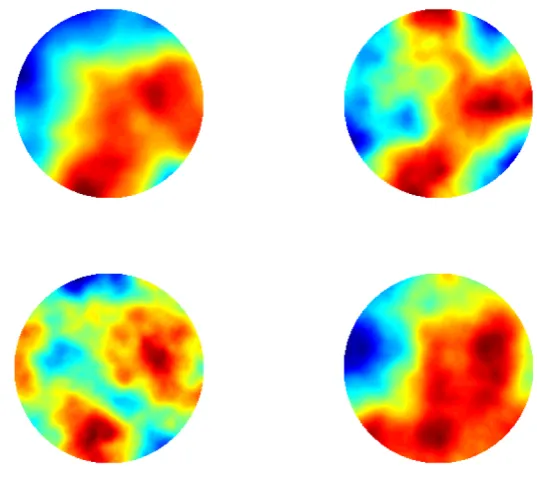
approach with Whittle-Mat´ern from four different initializations. . . 53 2.15 Model problem 1. EKI for the final iteration for the non-centered

method with level set from four different initializations. . . 54 2.16 Model problem 2. True log-permeability. . . 55 2.17 Model problem 2. Progression through iterations of non-hierarchical

(9)

2.18 Model problem 2. Progression through iterations of centered hierar-chical method. . . 57 2.19 Model problem 2. Progression through iterations of non-centered

hierarchical method. . . 58 2.20 Model problem 2. Progression of average value for α1 and τ1. . . . 58

2.21 Model problem 2. Progression of average value for α2 and τ2. . . . 59

2.22 Model problem 2. Left: relative error. Right: log-data misfit. . . 59 2.23 Model problem 2. EKI for the final iteration for the non-centered

approach from four different initializations. . . 60 2.24 Model problem 3. Progression through iterations of non-hierarchical

method. . . 61 2.25 Model problem 3. Progression through iterations with hierarchical

Gaussian random field. . . 62 2.26 Model problem 3. Progression through iterations with hierarchical

Cauchy random field. . . 62 2.27 Model problem 3. Left: relative error. Right: log-data misfit. . . 63 2.28 Model problem 3. EKI for the final iteration for the Gaussian

hier-archical method from four different initializations. . . 63 2.29 Model problem 3. EKI for the final iteration for the Cauchy

hierar-chical method from four different initializations. . . 63 3.1 Performance of hierarchical localization. Left: reconstruction of the

truth. Right: learning rate of the length-scale. . . 86 3.2 Performance of hierarchical covariance inflation. Left: reconstruction

of the truth. Right: learning rate of the length-scale. . . 87 4.1 Left: spare grid training set in [−1,1]2_{. Right: LOPs training set in}

[−1,1]2 _{. . . 104}

4.2 RBM numerics. Orthonormalized snapshots for LOPs in [−1,1]1_{. . . 105}

4.3 RBM numerics. Left: FEM solution. Right: RBM solution. . . 106 4.4 RBM numerics. Associated errors for Lebesgue optimal points in

[−1,1]1_{. . . 106}

4.5 RBM numerics. Parameter selection for Lebesgue optimal points in [−1,1]1_{. . . 107}

4.6 RBM numerics. Errors with respect to our snapshots in [−1,1]1_{. . . 107}

(10)

4.9 2D RB-EKI numerics. Left: True permeability. Centre: Finite

ele-ment reconstruction. Right: Reduced basis reconstruction. . . 115

4.10 2D RB-EKI numerics. Left: RB-relative error. Right: RB-log-data misfit. . . 115

5.1 Representation of the eikonal equation. . . 128

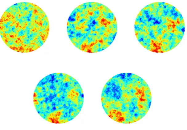
5.2 Random draws from the KL expansion with`= 0.1 andα= 1.5,2.5,3.5 and 4.5 with a fixedσ = 1. . . 132

5.3 Random draws from the KL expansion withα= 3 and`= 0.1,0.05,0.02 and 0.01 with a fixedσ = 1. . . 133

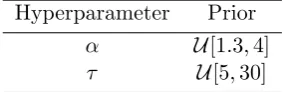
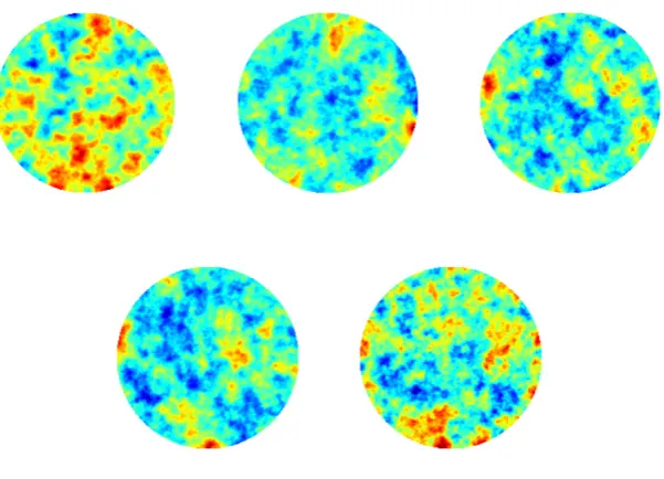
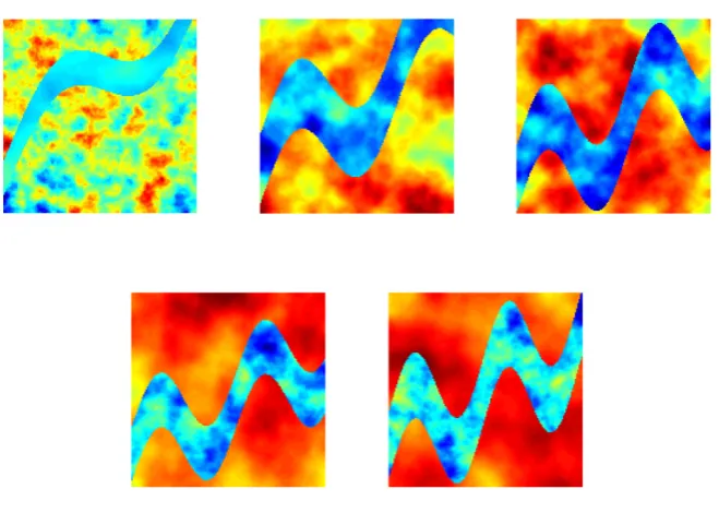
5.4 Random draws from level set thresholding of three interfaces from Gaussian draws with varying regularity and length scale with three interfaces. . . 136

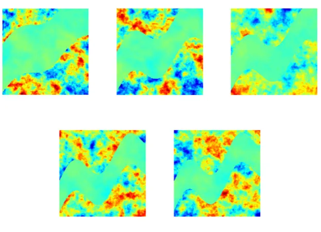
5.5 Random draws from vector level set thresholding with varying regu-larity and length scale with three interfaces. . . 137

5.6 Random draws from circular fixed shape prior with varying positions and radii. . . 138

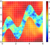
5.7 Top row: various slowness functions of priors. Bottom row: corre-sponding forward solution. . . 139

5.8 Learning rates of hyperparameters. Left: α. Right: `. . . 148

5.9 Hierarchical truth. . . 149

5.10 Reconstruction of hierarchical prior. . . 149

5.11 Final iteration from four different initializations of hierarchical prior. 150 5.12 Hierarchical prior. Left: Relative error. Right: Log data misfit. . . . 150

5.13 Vector level set truth. . . 152

5.14 Reconstruction of vector level set prior. . . 152

5.15 Learning rates of hyperparameters. Left: α. Right: `. . . 153

5.16 Vector level set prior. Left: Relative error. Right: Log data misfit. . 153

5.17 Final iteration from four different initializations of vector level set prior.154 5.18 Fixed shape truth. . . 155

5.19 Reconstruction of fixed shape prior. . . 155

(11)

Acknowledgments

A PhD is a long journey and process where numerous people have helped in different ways. First and foremost I would like to thank my primary supervisor Prof. Andrew Stuart. It was Prof. Stuart who introduced me to the interesting areas of Bayesian inverse problems and data assimilation, and who helped with attaining an EPSRC industrial studentship. Under his supervision I developed and enhanced both my research and interpersonal skills, and for that I am deeply indebted to him. I could not have asked for a better supervisor.

(12)

and comments, and also for their flexibility on the timing of the viva examination. The progression of this thesis would not be possible without industry funding from both E.ON and Premier Oil, for which I thank Dr. Jonathan Carter and Patrick Jennings.

Outside of research many people have made the PhD transition easier, in-cluding office mates and friends from before, in particular: Anil, Adam, Ati, Barri, Daniel, Dave, Jakub, Lloyd, Michael, Michael. H, Rohan and Wojciech.

(13)

Declarations

This thesis has been submitted to the University of Warwick in support for my application for the degree of Doctor of Philosophy. This is a confirmation that this thesis is the sole work of the author. I hereby declare that this thesis does not in-clude any previous material that has been submitted by a researcher for publication without acknowledgment.

A number of pieces of literature have been produced from this work, which are included in this thesis. A list of submitted papers, and ones that are in preparation, are provided below.

• N. K. Chada. Analysis of hierarchical ensemble Kalman inversion,

submitted to Journal of Inverse and Ill-Posed Problems.

• N. K. Chada, C. M. Elliott, K. Deckelnick, A. M. Stuart and V. Styles, A Bayesian formulation of the inverse eikonal equation,in preparation.

• N. K. Chada, M. A. Iglesias, L. Roininen and A. M. Stuart. Parameterizations for ensemble Kalman inversion,Inverse Problems, 34, 2018.

(14)

Abstract

(15)

Chapter 1 Background

1.1 Introduction

In numerous scientific disciplines inverse problems are ubiquitous. Inverse problems [138] are concerned with the recovery of an input to a model, or set of equations, from partial noisy measurements of an output. Some examples of common inverse problems include inferring the geological properties of an oil reservoir from produc-tion data, calculating the earths density from its gravity fields and estimating the sound speeds in the earth’s subsurface from seismic data. Mathematically speak-ing inverse problems can be expressed as aimspeak-ing to estimate u ∈ X from noisy measurements of datay∈ Y which are in the form

y =G(u) +η, (1.1.1) where

• X,Y - function spaces.

• u∈ X - input.

• y∈ Y - output.

• G :X → Y - forward operator.

• η - additive noise.

Usually we assume that (X,k · kX),(Y,k · kY) are two Banach spaces and our output,

(16)

noise are possible; however in this thesis we will focus on additive Gaussian noise for simplicity. An issue that arises when aiming to solve the inverse problem (1.1.1) is that it is ill-posed in the Hadamard sense i.e. there is no guarantee of existence, stability and uniqueness of solutions. Due to this drawback during the 20th_Century

mathematicians aimed at producing algorithms that approximated a solution to (1.1.1). An idea that came about was that one way to approximate the solution to inverse problems was by relating it it to the least squares functional

ΦLS(u) =

1 2

y− G(u) 2

Y , (1.1.2)

with subscript LS denoting least squares. From (1.1.2) our solutionu∗ to the inverse problem is then given by a minimisation procedure such that

u? = argmin

u∈X

ΦLS(u),

where our minimization occurs in the solution spaceX. However, despite this for-mulation with the LS functional there still lies issues with approximating a solution. We can approximate solutions, but under certain conditions uniqueness is not guar-anteed as well as the stability of solutions. One way that was proposed to overcome this issue was to modify the least square functional such that it incorporated prior information of the unknown. By doing so this leads to a slight modification of (1.1.2), where now our functional is defined as

ΦTP(u) =

1 2

y− G(u) 2

Y +R(u). (1.1.3)

Our new inclusion in our least-square functional is a regularisation termR(u). One example of this is the form ofR(u) = λ₂|u|2

Z; this is referred to as Tikhonov-Phillips

regularization [55, 107]. From our regularisation term λ >0 denotes our regulari-sation constant and Z is an embedded subspace of X. The motivation for adding regularisation terms is threefold: firstly to aid the inversion by reducing the amount of influence the data has on the solution, i.e. to prevent overfitting of data. Sec-ondly the add some further prior information about our unknown. Finally adding regularization ensures that the inverse problem is continuous with respect to the data. Choosing the form of regularization can be dependent on the actual problem of interest for inversion and model [13,54]. Now we can restate our inverse solution which is the following minimization procedure

u?= argmin 1

y− G(u)2

+λ|u|2

(17)

As there is a relationship between the TP functional and LS functional, optimi-sation methods have been traditionally been used and applied for solving inverse problems in the form of (1.1.4). Some common examples of iterative optimisation algorithms that have been used include: the Gauss-Newton method [12, 131], the Landweber method [65, 125] and the conjugate gradient method [85]. Like many optimizations methods, solving inverse problems requires information about deriva-tives. In the inverse problem setting this would include the JacobianDG(u) and the HessianD2_G₍_u_{), which are based on the forward operator. There has been extensive}

research into deterministic inverse problems which have included various forms of regularization. Although this aids with approximating stable solutions, still does not resolve the lack of uniqueness. Resolving this issue largely depends on the in-verse problem, the setting and the form of regularization which is added. One way to alleviate this issue is to look at an alternative approach that was adopted to solve inverse problems. This approach negates the idea of characterizing a functional and aiming to minimize it foru. Instead the unknown u is set as a probabilistic distri-bution, where all the quantities from (1.1.1) are treated as a random variable. This approach is known as a statistical or Bayesian approach to inverse problems.

1.2 Bayesian Approach

The methodology that was discussed previously in subsection 1.1 is related to the “deterministic approach” to inverse problems. Since then there has been much development in this field which has sparked an alternative viewpoint of inverse problems. Instead of our unknown u we are now interested in characterizing a distribution of the random variable u|y which is the unknown conditioned on the noisy datay. This is statistical view point of inverse problems which is commonly referred to as the “Bayesian approach” [87,137]. Taking our inverse problem (1.1.1) the Bayesian approach allows us to treat each quantity as a random variable with a Lebesgue density. In order to characterise our new unknown we apply Bayes’ Theorem which, in its general finite-dimensional form, is

P(u|y) = P(u, y)

P(y) (1.2.1) P(u|y) = P(y

|u)×_P(u)

P(y) (1.2.2)

(18)

In (1.2.3) the termP(u) denotes ourprior distribution, encoding initial belief about

our unknownu, prior to seeing any data; on the other hand thedata-likelihood term

P(y|u) captures the relationship between the forward modelG(u) and the datay. By

using Bayes’ Theorem, as done in (1.2.2), we can combine both theprior and data-likelihood which results in the conditional distribution ofugiveny,P(u|y), known as

theposterior. The form (1.2.3) is presented because the constant of proportionality

P(y) is often hard to compute, and is not needed for many computational methods

which explore the posterior. We note that in the case of our posterior form (1.2.3) we can approximate the posterior up to some level of proportionality. In many scenarios in Bayesian statistics the normalising constant 1

P(y) is not known, or is

to difficult to obtain. However, despite this simple form of Bayes’ Theorem, the Bayesian approach has been further applied to inverse problems in a differential equation setting, specifically partial differential equations (PDEs). Due to this one has to reformulate Bayes’ Theorem for PDEs, in a function space setting. Instead of a distribution we now wish to characterise our unknown as a posterior measure

µy_{. This change corresponds to going from a finite-dimensional to a}_∞_-dimensional

problem. An obvious question to ask is what advantages does the Bayesian approach have over the deterministic case? Unlike its counterpart, under certain conditions, well-posedness of the Bayesian inverse problem can be attained. This is one of the key significant advances with the Bayesian approach, which is possible due to its ∞-dimensional analysis. Secondly, arguably its main contribution is handling uncertainty within the problem. This can be tackled more effectively due to various prior forms, where a range of these are discussed in [137]. However much of the initial and existing theory on this assumed that the reference measure was of a Gaussian form. We now recall the definition of a Gaussian measure [20] and discuss some important definitions and assumptions which are required in order to present a well-posedness theorem of (1.1.1).

Definition 1.2.1. A Borel measure µ on R is called a non-degenerate Gaussian measure if there exists a m∈_R andσ2 _>₀ _{such that}

dµ dλ(x) =

1

√

2πσ2 exp

− 1

2σ2(x−m) 2_.

A Gaussian measure can be characterized through two quantities its mean

m∈_R and its variance (covariance) σ2 _>_{0. We now extend this formal definition}

to Gaussian measures on Banach spaces.

(19)

all`∈ X∗_.

From the above definition`#_µ _{is a push forward measure of the measure}_µ_.

We say thatµis centered if`#_µ _{has mean 0 for all}_`_{∈ X}∗ _{. Our final definition on}

Gaussian measures is with regards to defining the covariance of a Gaussian measure on both a Banach and Hilbert space.

Definition 1.2.3. Let µ be a centered Gaussian measure on a separable Banach spaceX. Then the covariance operator C:X × X →R is defined as

C(`, `0) =

Z

X

`(u)`(u0)µ(du), (1.2.4)

is called the covariance operator ofµ. IfX is a Hilbert space, then after identification

with its dual space, our covariance operator is now

C=

Z

X

(u⊗u)µ(du).

In the case of a centered Gaussian measure µ ∼ N(0,C), the measure is defined entirely through its covariance operator. In the context of Bayesian inversion in the∞-dimensional case an important question is how to relate a measure on the prior µ0 to the posterior measure µy. With Gaussian measures this relationship

between both measures could be represented through a Radon-Nikodym derivative

dµy dµ0

(u) = 1

Z exp(−Φ(u;y)). (1.2.5)

The Radon-Nikodym derivative (1.2.5) describes the change of measure from the prior to the posterior, and as seen through Bayes’ Theorem (1.2.3), this is achieved through the negative log-likelihood, which in this case is Φ(u;y) up to a constant

Z. To express this change of the measures, we require that µy _{to be absolutely}

continuous with respect to the measure µ0. In order to provide a well-posedness

theorem for the posterior measureµy _{we need a suitable metric to provide a stability}

result. Common metrics which are used are the total variation, the Hellinger and Kullback-Liebler metric [91].

Definition 1.2.4. (Total variation distance) Given two measures µ and µ0, and their corresponding densities ρ(u) and ρ(u0₎_{, the total variation distance between} these measures is given as

dT V(µ, µ0) =

1 2

Z

Rn

(20)

Definition 1.2.5. (Hellinger distance) Given two measuresµandµ0_{, and their} cor-responding densities ρ(u) and ρ(u0), the Hellinger distance between these measures is given as

dHell(µ, µ0) = 1

2

Z

Rn

p

ρ(u)−pρ0₍_u₎2_du1/2_.

Definition 1.2.6. (Kullback-Liebler divergence) Given two measuresµandµ0, and their corresponding densitiesρ(u)andρ(u0₎_{, the Kullback-Liebler divergence between} these measures is given as

dKL(µ0||µ) = Z

Rn

log

ρ0₍_u₎

ρ(u)

ρ0(u)du.

An important way to compare some of these metrics is through the following relationship between the total variation and Hellinger metrics

0≤ √1

2dT V(µ, µ)≤dHell(µ, µ

0₎_≤_d

T V(µ, µ0)1/2 ≤1.

A natural question one can ask regarding the above metrics is between the total variation and Hellinger metric, which one is preferred? The following lemma is crucial in understanding why the Hellinger distance is more favourable over total variation.

Lemma 1.2.1. Let f :Rl→Rp be such that Eµ|f(u)|2+Eµ

0

|f(u)|2 <∞.

Then

Eµf(u)−Eµ 0

f(u)

≤2 Eµ|f(u)|2+Eµ 0

|f(u)|21₂

dHell(µ, µ0), where as a consequence

Eµf(u)−Eµ 0

f(u)

≤2 Eµ|f(u)|2+Eµ 0

|f(u)|21₂

dT V(µ, µ0)1/2.

Lemma 1.2.1 is significant as it shows that two measuresµand µ0 areO( )-close within the Hellinger metric. That is if the functionf(u) is square integrable with respect toµ and µ0_{, then its expectations are}_O₍_{)- close within the Hellinger}

metric. However this is not the case with the total variation metric as the expecta-tions off(u) with respect toµandµ0areO(−1/2_{). In order to attain}_O₍_)-closeness

we need stronger assumptions, which is achieved through the following lemma.

(21)

µ0_{, where we denote the almost sure upper bound on}_|_f_|_by _f

max, then

Eµf(u)−Eµ 0

f(u)| ≤2fmaxdT V(µ, µ0).

The previous two lemmas are proved in [91], and provide a basis on why we should choose the Hellinger metric over the total variation. This is due to the induced perturbations of the measure on expectations of square-integrable functions. It is for this reason why we consider the Hellinger metric as a more “appropriate” metric to use than total variation for the existence of solution to a Bayesian inverse problem. We omit using the Kullback-Liebler (KL) divergence as using the definition of a metric, it does not abide by the symmetry property of the metric. As we have discussed both necessary concepts we can present the following theorem which provides uniqueness and existence of solutions to (1.1.1), which is based on the Hellinger metric.

Theorem 1.2.1. (Well-posedness) Assume that µ0 is defined as N(0,C), y by

(1.1.1) and Φ by 1₂|y− G(u)|2

Γ. If µy is the regular conditional probability measure onu|y, then µy _µ

0 with Radon-Nikodym derivative

dµy dµ0

(u) = 1

Z exp(−Φ(u;y)), where

Z :=

Z

X

exp(−Φ(u;y))µ0(du).

Furthermore µy _{is locally Lipschitz with respect to} _y _{in the Hellinger distance: for}

ally, y0 with max{|y|Γ,|y0|Γ} ≤r, there exists a C=c(r)>0 such that dHell(µy, µy

0

)≤C|y−y0|_Γ.

Remark 1.2.1. We note that with the above theorem, we have assumed that our prior is of a Gaussian form. This theorem can be extended to include numerous other priors such as uniform and Besov, whilst the main statements of the theorem

still hold. Further assumptions are required for well-posedness which can be found

in [137].

(22)

meth-ods which arise in a deterministic optimization setting. We will discuss both the numerical method used in its original context and how the methodology can be used for solving Bayesian inverse problems. These methods will primarily be split into data assimilation methods and Markov chain Monte Carlo methods, whilst we briefly review other commonly used methods.

1.3 Markov Chain Monte Carlo Methods

In many situations arising in computational statistics one is interested in simulating from a probabilistic distributionπ, or in other words calculating an expectation of aπ- integrable functionf :X →_R

Eπ(f) := Z

X

f(x)π(dx). (1.3.1) However simulating from a distributionπ is not always possible due to a number of reasons that make it difficult such as:

• High dimensionality of the problem.

• Difficult to attain the normalising constant.

Traditional methods such as analytical integration and quadrature schemes do not aid significantly when aiming to solve (1.3.1). One way to overcome this issue is to construct a Markov chain{Xi}n_i₌₁ on a measurable space (X,B(X)), with Borel σ-algebra that converges toπ. This in a nutshell is the aim of Markov chain Monte Carlo (MCMC) methods [121], where we are interested in constructing an invariant ergodic Markov chain with respect to π. MCMC methods are used to calculate (1.3.1) based the notion of ergodic averages

Sn(f) :=

1

n n X

i=1

f(Xi), forn∈R+.

We know from the strong law of large numbers that the ergodic average, taking a large enoughn, will converge to π i.e.

Sn(f)−→Eπ(f), when n→ ∞.

From the central limit theorem (CLT) we know that the convergence is of order

O(n−12), which is also the order of MCMC methods. By working in an MCMC

(23)

(1.3.1), and as a result can obviate the need to calculate the normalizing constant. One of the most common type of MCMC methods that are used in practice are Metropolis-Hastings (MH) algorithms. These algorithms are based on an accept-reject scheme for proposed moves through a transition kernelq(x, y), which encodes the condition that the probability of going from statex toy is the same as from y

tox. It implies that π is an invariant distribution for Markov chain with kernelq. The accept-reject is designed in such a way to allow for detailed balance

π(y)q(y, x) =π(x)q(x, y). (1.3.2) This detailed balance (1.3.2) is a consequence of reversibility of the Markov chain, and it reflects the property that the probability of going from state x to y is the same as fromy tox. The MH algorithm is described in more detail in Algorithm 1. We recall the properties of transition kernels through the following definition.

Definition 1.3.1. A function q :X × B(X)→ [0,1]is defined as a Markov kernel if the following conditions are satisfied

• For each x∈ X, q(x,·) is a probability measure on(X,B(X)).

• x7→q(x, A) isB(X)-measurable for all A∈ B(X).

In the context of MH from (1.3.2) we can think ofπ(y) as the target density we are interested in simulating from andq(x, y) as the transition kernel, or proposal, from the current state x to y. The accept-reject scheme for MH is based on an acceptance probability which is given in the form

α(x, y) := minn1,π(y)q(y, x) π(x)q(x, y)

o

, forx6=y,

For the MH algorithm the overall kernel for the scheme can be written as,

p(x, y) =α(x, y)q(x, y) + (1−α(x, y))p(x, y). (1.3.3) which includes the usual transition kernelq(x, y). The intuition behind the (1.3.3) is that we have a number of choices based on proposing and accepting y. If we move from x to y and the proposed move is accepted then we have the result of

(24)

Algorithm 1 Metropolis Hastings Algorithm

1. If current position isx propose move to y according to q(x, y).

2. Compute acceptance probability

α(x, y) = minn_ππ(₍_xy)₎q_q(₍y,x_x,y₎),1o, forx6=y.

3. With acceptance probability α(x, y) move from from x to y otherwise stay still.

4. Go back to 1.

For MH we can choose a number of proposals which work best under different scenarios. Three common proposal types are given by:

• Random walk Metropolis Hastings (RWMH).

• Metropolis-adjusted Langevin algorithm (MALA).

• Preconditioned Crank-Nicholson (pCN).

For RWMH this employs a Gaussian proposal that is centered at the current state. Given we are atxn the proposal for the next step is defined as

yn+1 =xn+σξn+1, (1.3.4)

such that ξn+1 ∼ N(0, σ2). Our initial state x0 ∼ N(0,1) is also normally

dis-tributed, which implies our transition kernel is now q(x, y) ∼ N(x, σ2_{). Due to}

symmetry of the Normal distribution we can set the proposal as q(x, y) = q(y, x) which leads to an acceptance probability of

α(x, y) := minn1,π(y) π(x)

o

. (1.3.5) An important note to make about RWMH is that the noiseξn+1 is independent of xn, which means that the noise has no information about the current position. This

is one limitation regarding this proposal. An obvious way to alleviate this problem is to consider more informative proposals. This leads to an alternative method that combines more information, while remaining in the MH accept-reject mechanism. One example of this is the MALA proposal [63,122]. Its derivation comes from the SDE

(25)

which is a common stochastic differential equation (SDE) that arises in various scientific disciplines, known as the Langevin equation. From (1.3.6) {Wt}t≥0 is a d-dimensional standard Brownian motion, V(x) is a potential with Xt ∈ Rd and β >0 is a constant. In order to encapsulate Langevin dynamics in our MCMC we need to efficiently discretize (1.3.6). Arguably the simplest way to do so is by taking a forward Euler discretization of the SDE (1.3.6)

Xn+1 ∼ N(Xn−h∇V(Xn),2hId),

with our constant chosen asβ = 1. Therefore the proposal of MALA are given as

Yn+1:=Xn−h∇V(Xn) + (2h)1/2ξn+1, ξn+1∼ N(0,1). (1.3.7)

Based on the MALA proposal given in (1.3.7) our transitional kernel is nowq(x, y)∼ N(x−h∇V(x),2hId). Our final proposal we discuss is a simpler variant of the

RMWH which includes a slightly different proposal kernel to that of (1.3.4). The proposal itself is a redefined version of RWMH given as

yn+1 =m+ (1−β∗2)1/2(xn−m) +β∗ξn+1, (1.3.8)

which we call the pCN method. Here again we assume that ξn+1 ∼ N(0,C) is

Gaussian noise, but with the addition ofβ∗∈(0,1] which is some tuneable parameter

and m is the mean of our initial state. Equation (1.3.8) was first derived in [18] and tested numerically in [39]. The pCN proposal is specific to when our target density is a Gaussian. The intuition behind the parameterβ∗ is that in this context

it is defined as the proposal variance and can be tuned to ensure a more reasonable acceptance probability. Combined with the initial conditionx0it can be viewed as an

improvement over the independence sampler, that is defined through the acceptance probability (1.3.5).

1.3.1 MCMC Within Inverse Problems

(26)

1.2.1.

Notably the work of Roberts and Stuart [17, 104, 118] developed much of the existing literature of various MCMC algorithms in high dimensions, and this itself posed a motivation for merging this work to the Bayesian approach. Much of the existing work has been based on the RWMH, whereas before, the key aspects of this in Bayesian inversion is through the proposal and the likelihood. Recalling that pCN proposal is defined, with slightly different notation

ˆ

u(n)= (1−β∗2)1/2u(n)+β∗ζ(n), ζ(n)∼ N(0, C). (1.3.9)

We omit defining our proposal as y as this denotes the data. As we assume our prior measure µ0 is a centered Gaussian measure, we set m = 0 .We can interpret

the proposal (1.3.9) as how we define our prior which is given through ζ(n) _with

covarianceC. Now for the data-likelihood, this is incorporated in the MH framework through the acceptance probability which is given by

α(u(n),uˆ(n)) := minn1,π(ˆu) π(u)

o

= min

1,exp Φ(u(n)_;_y₎₋_Φ(ˆ_u(n)_;_y₎ _. _(1.3.10)

Combining both the proposal and the acceptance probability a simple RMWH al-gorithm for Bayesian inversion is presented below in Alal-gorithm 2.

Algorithm 2 pCN Algorithm

1. Set initial state u(n)_{∈ X} _{with proposal (1.3.9) with} _β

∗∈(0,1].

2. Compute acceptance probability

α(u(n),uˆ(n)) = min

1,exp Φ(u(n);y)−Φ(ˆu(n);y) .

3. With acceptance probability α(u(n)_,_u_ˆ(n)_{) move from} _u _{to ˆ}_u _{otherwise stay}

still.

4. Go back to 1.

(27)

[80] and level set techniques [81].

In this context we can state that this particular inverse solver is a sampling method as it gains inference from a probability distribution in the form of a posterior through (1.3.3). As we will discuss later, there are other types of methods that can be used in a Bayesian setting such as methods deriving from optimization rather than sam-pling.

1.4 Data Assimilation Techniques

Data assimilation [57,90,91] is the study of state estimation of a dynamical system with the incorporation of noisy measurements. The ideas behind data assimilation can be related back to control theory and optimal control [88]. Since then there has been a growing number of applications where data assimilation techniques can be used such as weather forecasting, geosciences and meteorology [58,59]. The two governing equations of data assimilation, in discrete time, are given as

uj+1 = Ψ(uj) +ξj, {ξj}j∈_Z+ ∼ N(0,Σ), (1.4.1) yj+1 =H(uj+1) +ηj+1, {ηj+1}j∈_Z+ ∼ N(0,Γ). (1.4.2)

Here{uj}j∈Z+ is our signal which is updated through a forward operator Ψ :R

m_→

Rm, which when combined with noise, provides the update uj+1. Our data is

de-noted asyj+1which is produced by sending our updated signal through the operator H:Rm →Rn which is known as observational operator. Our initial conditions for

the system are given as u0 ∼ N(m0,C0). We also notice that there is the

addi-tion of additive Gaussian noise. In data assimilaaddi-tion the common goal is to use the data (1.4.2) to inform the signal dynamics governed by (1.4.1). We can think of this probabilistically where we are interested in characterising the distribution of P(uj|yj). Algorithms that are used to quantify this distribution are classified as

either; (i)smoothing, (ii)filtering.

Smoothing is concerned with determining the smoothing distribution P(u|y) ∝ P(y|u)P(u) where the signal is conditioned on all of the data specified in the

ap-propriate time interval. Filtering is concerned with the determining the filtering distribution P(uj|Yj) where Yj = {yl}j_l₌₁ be the accumulated data up to time j.

Filtering is commonly split into two steps:

• Prediction step: P(uj|Yj) 7→ P(uj+1|Yj) - maps the signal into the data

space.

(28)

comparing it with the data.

By applying Bayes Theorem’ in the analysis step we can deduce that

P(uj+1|Yj+1) =P(uj+1|Yj, yj+1)

= P(yj+1|uj+1)P(uj+1|Yj)

P(yj+1|Yj)

(1.4.3) Unlike smoothing, filtering has the advantage of determining information from the signal at the current state. Due to this filtering algorithms are a more popular choice among practitioners. Some of the most common filtering algorithms that are used are: (i) the Kalman filter, (ii) the extended Kalman filter (ExKF), (iii) 3DVAR and (iv) the ensemble Kalman filter (EnKF). A common attribute among filtering algorithms is to update the signal based on observations through statistical quantities. As the original signals that were considered were Gaussians i.e. uj ∼

N(mj, Cj), we aim to update our filtering distribution using notions of the mean

and the covariance. Below we present the 3DVAR algorithm and the extended and ensemble Kalman filter.

1.4.1 3DVAR

The 3DVAR algorithm is derived from the linear Kalman filter [88], which has the assumption that the underlying signal is of a Gaussian form. It differs in that the covariance matrix is fixed such that ˆCj+1≡Cˆ. This leads to the equations

ˆ

mj+1= Ψ(mj),

mj+1= (I−KH) ˆmj+1+Kyj+1, K= ˆCHTS−1,

S=HCHˆ T + Γ.

3DVAR works in a variational manner and is sequentially updated at eachj

through the minimization procedure ˆ

mj+1= argmin u

In(u),

with cost functionIn(u) given as In(u) :=

1

(29)

This optimization procedure despite having a different mathematical formulation, leads to the update formulae for the ExKF. As suggestive from its name in practical application the minimisation procedure is taken over all spatial dimensions. The extension from this is 4DVAR which takes the time dimension into consideration. However by doing so our problem is now given as a smoothing algorithm. We now look to go beyond this with two methods that sequentially update our quantity of interest through both an updated mean and covariance; the extended Kalman filter and ensemble Kalman filter.

1.4.2 Extended Kalman Filter

The ExKF was developed to work with non-linear Gaussian proposals of the linear Kalman filter which propagates both the mean and the covariances. As with all filtering methods the ExKF has a prediction and analysis step where the prediction step is to define both ˆmj+1 and ˆCj+1.

ˆ

mj+1 = Ψ(mj),

ˆ

Cj+1 =DΨ(mj)CjDΨ(mj)T + Σ.

Sj+1 =HCˆj+1HT + Γ, Kj+1 = ˆCj+1HTSj−+11 ,

mj+1 = (I −Kj+1H) ˆmj+1+Kj+1yj+1, Cj+1 = (I −Kj+1H) ˆCj+1.

In filteringKj+1 is commonly referred to as the Kalman gain matrix which describes

how much information we have gained through the covariance structure. From the predicted mean and covariance we have an update of our distribution in terms of

mj+1 and Cj+1.

1.4.3 Ensemble Kalman Filter

Out of the filtering algorithms that were mentioned in Section 1.4, the EnKF can be thought of as a Monte Carlo approximation of the Kalman filter which has certain advantages over its counterparts. Arguably its main advantage it acquires is the reduction in cost of the algorithm for high dimensional problems. As we can see with the ExKF we constantly have to update the covariances in the analysis step through previous knowledge of information. This procedure is expensive.

(30)

to represent the predicted mean and covariances, which in turn are used for the updated moments. As before, we can split the EnKF into a prediction and analysis step:

ˆ

u_j(n₊₁) = Ψ(u_j(n)) +ξ_j(n),

ˆ

mj+1 =

1

N N X

n=1 u(_jn₊₁),

ˆ

Cj+1 =

1

N−1

N X

n=1

(u(_jn₊₁) −mˆj+1)(u(_jn₊₁) −mˆj+1)T.

Kj+1= ˆCj+1HT(HCˆj+1HT + Γ), u_j(n₊₁) = (I−Kj+1H)ˆu_j(n₊₁) +Kj+1y_j(n₊₁),

y(_jn₊₁) =yj+1+η_j(n₊₁).

As before Kj+1 represents the Kalman gain matrix and ξj(n) and η (n)

j+1 are i.i.d.

Gaussian noise. In the EnKF context our prediction step defines a sample mean and covariance from our signal. From this in the analysis step we define our Kalman gain through our sample covariance, which updates our signal, which is given by u(_jn₊₁). This is aided by aiming to minimize the discrepancy of the datay(_jn₊₁) and the quantity

H(u). To better understand this discrepancy, there is an alternative approach of looking at the EnKF is through a variational approach, where we consider the follow cost function

In(u) :=

1 2|y

(n)

j+1−H(u)| 2

Γ+

1 2|u−uˆ

(n) j+1|

2 ˆ

Cj+1, (1.4.4)

for which we aim to minimise, which is defined as the updated mean ˆ

mj+1= argmin u

In(u). (1.4.5)

This minimization procedure relies on the updated covariance ˆCj+1 which is

depen-dent entirely on ˆv(n)_{. As described in the prediction step and update step of filtering,}

a mapping is presented between distributions. As we related the distributions in the filtering setting, for each step, we can do so similarly for the EnKF, i.e.

(31)

1.4.4 DA Techniques within Inverse Problems

Data assimilation and Bayesian inverse problems have an important connection, arguably due to the fact that both fields have a common aim of constructing a distribution of a quantity of interest conditioned on some data. In particular one data assimilation method that has seen a significant translation to inverse problems is the EnKF. We refer this type of inversion as ensemble Kalman inversion (EKI). EKI was first considered by Reynolds and coauthors [93,110] which was motivated by applications in subsurface flow. Since then a new method was proposed of how to effectively apply EnKF techniques to solve PDE-constrained Bayesian inverse problems. This was done through the work of Iglesias et al. [78, 79], known as the iterative EnKF method. This method proposed is very similar to that of the traditional EnKF, where in this context we are interested in updating an ensemble of particles{u(nj)}Jj=1 wherenis the iteration count andJ is the ensemble member.

This is achieved through defining the mean and the covariances ¯

G_n= 1

J J X

j=1

G(u(_nj)), (1.4.6)

¯

un=

1

J J X

j=1

(u(_nj)), (1.4.7)

C_nuw = 1

J−1

J X

j=1

((u(_nj))−u¯)×(G(u(_nj))−G¯), (1.4.8)

C_nww= 1

J−1

J X

j=1

(G(u(_nj))−G¯)×(G(u(_nj))−G¯), (1.4.9)

where as discussed before G is the forward operator of the PDE. Then finally the update of the ensemble is achieved through the following update formula

u_n(j₊₁) =u_n(j)+C_nuw(C_nww+ Γ)−1(y_n(j)− G(u(_nj))). (1.4.10) From the update formula (1.4.10) (y(j)_{− G}₍_u(j)

n )) can be viewed as the discrepancy

between the datayn(j) and the solution evaluated at the forward operator. Relating

this further to the EnKF discussed in subsection 1.4.3, our Kalman gain matrix in this context is simply Cuw

n (Cnww + Γ)−1. The iterative EnKF has two important

(32)

other is that the method can be viewed as asemi-Bayesian method in that it is based on an optimization framework, but can incorporate numerous Bayesian techniques, motivated from the likes of MCMC.

To derive this method we can do so in a number of ways, one is to follow a similar approach as the Kalman filter, was is shown in [88]. The other approach is to consider the functional of interest we aim to minimize as

I(u) =ky− Guk2_Γ+ku−u¯k2_C, (1.4.11) whereuTP is a solution of the functional (1.4.11). Equation (1.4.11) can be

charac-terized, as before, as the analysis step. An important result was shown in [92] that if we have a linear operatorG(u) =Gu, then for all cases of C,G,Γ we have

uTP = ¯u+CG∗(GCG∗+ Γ)−1(y− Gu¯),

whereG∗is the adjoint operator. By using the estimates (1.4.6) - (1.4.9) and update formula (1.4.10), and taking the limit as J → ∞, it was shown thatu →uT P. We

omit the derivation here but for the interested reader we refer them to [79]. One issue with this method, similarly with deterministic inverse solvers, is stability, where regularization is usually added. In the work of Iglesias [77] a regularized version was considered which was motivated by the work of Hanke [71] which looked at the effect of Levenburg-Marquardt regularization for nonlinear elliptic PDEs. This added an additional step to the iterative EnKF method in the form of a discrepancy principle (or stopping rule)

ky−G¯(u)k2_Γ ≤ζη, (1.4.12) whereζ >1/ρ∈(0,1) is a regularization parameter. Incorporating this regulariza-tion modifies our update equaregulariza-tion (1.4.10) to

u_n(j₊₁) =u_n(j)+C_nuw(C_nww+αnΓ)−1(yn(j)− G(u(nj))),

such thatαn≡αNn satisfies

ρkΓ−1/2(y(j)−G¯n)kY ≤αNnkΓ1/2(Cnww+αNnΓ)

−1₍_y(j)₋_G_¯ n)kY,

and where αn is chosen based on αin+1 = 2iα0n. By adopting this form of

(33)

was considered for tuning the additional parameters mentioned above.

The use of Levenberg-Marquardt regularization has been an effect tool in inverse problems, which originally arises from its use in nonlinear optimization. For a review on both the original Levenberg-Marquardt method, and its adaption as a form of regularization in inverse problems, we refer the reader to Appendix A.

We note as well that the discrepancy principle described as in (1.4.12) is just one possible choice one can use. This discrepancy principle arises from the Levenberg-Marquardt regularization, however once can choose other principles de-pending on the application or model problem. A nice review on discrepancy princi-ples can be found in the book by Hansen [72].

1.5 Other Computational Techniques

Our last two Bayesian inverse solvers that we aim to discuss differ in that one is of a Monte-Carlo form and the other is a variational method. The first one we will discuss is an extremely popular method used in computational statistics which are sequential Monte Carlo (SMC) methods.

1.5.1 Sequential Monte Carlo Methods

Gaining inference with respect to expectations from (1.3.1) can be difficult even with complex samplers. An alternative to using MCMC methods are SMC methods [42,43]. This is a convenient approach whenπ can be decomposed in a sequence of distributions, where importance sampling at each step can be implemented. These methods are based on hidden Markov models (HMM).

A HMM is composed of two processes which take values in measurable spaces (X,B(X)) and (Y,B(Y)). We assume we have a random variable {Xn}n≥0 which

take the form of a time-homogenous Markov chain with transition kernelmθ. Our

transition kernel depends on a set of parameters θ ∈ Θ. Our observed random variable{Yn}n≥1 are conditionally independent on and distributed according to

Yn|Xn∼gθ(·|Xn),

where we assume we have some initialX0 =x0 which is known. With SMC we are

interested in gaining inference fromπθ,y1:T

πθ,y1:T(f) = R

XTf(x1:T)QTn=1(xn−1, dxn)QTn=1gθ(yn|xn) l(θ;y1:T)

(34)

for some functionf :XT _→

Rwherel(θ;y1:T) denotes the likelihood forθsuch that l(θ;y1:T) :=

Z

XT T Y

n=1

mθ(xn−1dxn) T Y

n=1

gθ(yn|xn).

Likewise with data assimilation schemes, we can characterize SMC approaches as either smoothing or filtering methods. The simplicity of SMC methods depends hugely on the choice of the kernels. In the case of a Gaussian mθ and gθ we can

evaluate the likelihoodl(θ;y1:T) in analytical manner recursively. However the

con-verse of this with non-Gaussian kernels makes it more difficult where a number of algorithms have been developed. These include the bootstrap filter, the auxiliary particle filter, sequential importance resampling and more.

1.5.2 Maximum a Posteriori Estimation

An efficient and rather simple approach which is also considered in computational statistics are Maximum a posteriori (MAP) methods. The key idea behind these methods is based on quantifying the unknown target, which in this case is a posterior distribution, through its mode. The formal equation of a MAP estimator is

uMAP:= argmax

u P

(u|y).

MAP methods pose an advantage over maximum likelihood estimation (MLE)

uMLE:= argmax

u P

(y|u),

as it incorporates the prior distribution. However both MAP and MLE coincide when the prior is given as a constant function. Despite its simplistic approach MAP estimation can be viewed as a method which can perform significantly worse due a number of reasons. One of them is when the posterior is a multi-modal distribution it is not always a guarantee that the maximum value is a good estimate of the posterior. A second reason is that it is a point estimate, which is less informative than using a distribution to gain inference. For these reasons MCMC is a more favourable choice.

1.5.3 SMC & MAP Within Inverse Problems

(35)

and SMC methods. In the case of a linear inverse problem defined as

y=Au+η, η∼ N(0, Cη),

where A is linear operator andu∼ N(0, Cu) we can express our MAP estimate as P(u|y)∝P(y|u)P(u)

= exp(−1

2

C_u−1/2u 2

−

C_η−1/2(y−Au) 2

),

therefore leading to

uMAP= argmax u

exp(−1

2

C_u−1/2u 2

−C_η−1/2(y−Au) 2 ) , ⇐⇒ argmin u 1 2

C_u−1/2u 2

−

C_η−1/2(y−Au)

2 .

The Gaussian MAP estimate in the finite-dimensional case has been considered quite extensively which is summarised well in [46]. Extending this to the∞-dimensions we now think of a seeking a center of a ball with maximal probability and study the the limit of the center z as the radius δ tends to zero. This is aided through the Onsager-Machlup functionalI which satisfies

lim

δ→0

µ(Bδ₍_z 2)) µ(Bδ₍_z

1))

= exp(I(z1)−I(z2)),

such thatBδ₍_·₎_{⊂ X} _{is an open ball with radius}_δ_{. Since there has been development}

of MAP methods such as considering certain geometric priors [50] and extensions and more rigorous analysis [7,24].

In terms of SMC methods used for Bayesian inversion, there has been a number of papers developed which have analyzed this [16, 89] . However there still lacks an investigation on how these methods can be best optimized. This will of course depend on what particular SMC method is used. As the EnKF can be further seen as a HMM, the relationship between both methods could pose a nice combination for future work to be developed.

1.6 Outline of Thesis

(36)

understanding of PDE-constrained Bayesian inversion have been based on MCMC. Part of the reason behind this is that there are many problems in uncertainty quan-tification in which MCMC has been traditionally used, due to their high-level per-formance and for its sampling capabilities of a probability distribution. EKI is an optimization based alternative to MCMC which, like MCMC, operates via an en-semble, but has distinct computational advantages: it typically requires far fewer forward model evaluations.

Rather than focusing on understanding one aspect of EKI, the thesis is split into numerous avenues which answer different key and important questions in the field of inverse problems, but with the common theme that we aim to do so in a setting that aligns with subsections 1.4.3 and 1.4.4. In particular the motivation be-hind this thesis is to consider a number of avenues in EKI which are based on solving geometric inverse problems, i.e. where our underlying unknown contains some form of geometry, such as in the geosciences and in medical imaging. Examples include piecewise constant, piecewise continuous and level set functions. Understanding inverse problems through these functions is important as numerous fields require recovering some form of geometry such as geosciences and medical imaging. Some of the questions that this thesis aims to address are:

• Can we effectively use EKI to recover some form of geometry from our un-known, which includes various discontinuities?

• Given the computational burden that can arise with the forward operator, can we reduce this cost in a practical manner and what kind of cost reduction is possible?

• Can we transfer ideas from hierarchical Bayesian inversion to the EKI method-ology, and in doing so find improved inversion strategies?

• Given the current extent of the literature on Bayesian-related inversion, and the EKI in particular, can we extend this to new and potentially more chal-lenging PDEs applications?

The layout and description of each chapter is provided as follows:

1.6.1 Chapter 2. Parameterizations of Ensemble Kalman Inversion

(37)

unknowns where these additional unknowns correspond to hyperparameters which allow for parsimonious representation of the unknown, and which are learned from the data, along with the unknown itself. These priors are usually defined through three key parameters; (i) amplitudeσ∈_R, (ii) smoothness α∈_R+ _{and (iii) inverse}

length-scaleτ = 1/`∈R+ which appear in the covariance structureC

C=σ2₍_τ2_I₋_∆)−α_, _(1.6.1)

where ∆ is the Laplacian operator. However with EKI still lies a limitation which is known as the subspace property, that states however your prior is chosen, your reconstructed solution will be of a similar form. By placing a Gaussian initial ensemble with prescribed hyperparameters we can expect our end result to have a similar result with the same value of hyperparameters. One technique we use to break away from this property is to generate the Gaussian prior through a Stochastic partial differential approach, which in turn states that the solutionu of

(τ2_I_{− 4}₎α₂_u₌_τ−2/dp βξ,

omits a structure similar to that of the covariance (1.6.1). By doing so we can successfully break away, and effectively learn the various unknowns. This is based on two hierarchical approaches: the centered and non-centered case. We consider this for a variety of PDEs and adopt level set techniques. A further extension we look at in this chapter is the question of whether we can extend the modelling of our hyperparameters from a scalar field to a random field, as done with our underlying unknown. For this we adopt the length-scale as both a Gaussian random field, but also a newly adopted random field in the area of Bayesian inversion, a Cauchy random field. The latter poses an advantage over the former as it performs better for edge-preserving and rougher features. We further consider analyzing some limit analysis of hierarchical EKI which can be seen as an extension for the recent work that was done on non-hierarchical EKI.

(38)

1.6.2 Chapter 3. Analysis of Hierarchical Ensemble Kalman Inver-sion

The EnKF has showcased a high level of applicability to a number of scientific dis-ciplines, due to its ease of implementation and low computational cost. However despite this is a lack of clear foundational understanding, both for the traditional EnKF from data assimilation, and EKI for inverse problems.. Much of the work since the derivation of the work has been on improving the algorithm under dif-ferent settings. Only till recently there has been some work which has aimed at understanding this. However for EKI there has only been one piece of work that has looked at developing diffusion limits aiming to understand the long-term be-haviour. This chapter aims to complement Chapter 2. in that it provides a more analytical understanding of hierarchical EKI. We look to extend the results of the work done on EKI, namely understand the long-term behaviour. It was shown that in the linear case EKI could be interpreted as a gradient-flow structure. In the hier-archical case we see that this also holds, for both the centered and non-centered case. Aside from diffusion limits and gradient-flow structures, we aim to prove whether using both approaches allow us to break away from the subspace property, in the case of both a discrete and continuous case. Finally we consider hierarchical aspects of certain variants of the EnKF, which include localization and variance inflation. Both these techniques are known to break from the induced property, therefor we take a hierarchical approach and see if if we have the similar effect if not a better performance. This is highlighted through a numerical example on a 1D linear elliptic PDE.

This chapter was solely carried out by myself, and has been submitted as the solo-authored paper [31]. However the work benefitted from a number of individuals including Dr. Marco Iglesias and Prof. Claudia Schillings.

1.6.3 Chapter 4. Reduced Basis Methods for Bayesian Inverse

Problems

(39)

been developed to tackle these issues. These methods are commonly referred to as reduced order models (ROMs). One of these methods, which we consider in this chapter, are reduced basis methods (RBMs). RBMs can be interpreted as a dimension reduction method based on a Galerkin projection which is based on a greedy algorithm. The solution of the RBM is controlled via an a posteriori error bound. It is specific to parameterized PDEs, which are PDEs where the input and output are induced by some random parameter. As an example in an elliptic PDE we would have both a random diffusion coefficient κ(x;ϑ) and a random solution

p(x;ϑ) induced by some parameter ϑin a parameter space Γ, given by

−∇ ·(κ(x;ϑ)∇p(x;ϑ)) =f, ∈D, p(x;ϑ) = 0, ∈∂D.

The RBM projects the solution pN onto a smaller space XN and aims to build a

RB space by solving the following system given by the variational formulation

A(pN, q;ϑ) =F(q), ∀q ∈XN.

The focus on this chapter is two fold; firstly that we consider the proposal of a new set of points to represent the parameter space Γ. Traditional choices of these points include uniform points, random points and Curtis-Clenshaw points. Our set of points we propose are Lebesgue optimal points, where our motivation arises from the work of Chen et al. [35]. By using these points we aim to see if we can get more accurate results and see how these points scale within our experiments. The second aim of this chapter is to transfer these ideas from ROMs, and apply them in to Bayesian inverse problems. Specifically we consider the inverse problem of Darcy flow, where in particular we focus on geometric inverse problems such that our random coefficient takes a piecewise constant form. We briefly consider the inverse problem of impedance tomography where we derive particular bounds related to the RBM.

(40)

1.6.4 Chapter 5. A Bayesian Formulation of the Inverse Eikonal Equation

Since the development of the Bayesian approach in the infinite dimensional case, there have been a wide class of PDE-related inverse problems that have been ana-lyzed. Most of this work has been concerned with elliptic and parabolic problems, such as those arising in groundwater flow, electrical impedance tomography and electro-magnetics (elliptic) and data assimilation in fluid, through the Navier-Stokes equation (parabolic). One class of PDEs that has a rich theory behind it, but has not being analyzed greatly in an inverse setting, are Hamilton-Jacobi (HJ) equations. We are interested in one particular HJ equation which is the eikonal equation. The eikonal equation is an important PDE which arises in numerous application such as computer vision and geosciences. The forward problem is concerned with findingT

solving

|∇T(x)|=u(x) x∈Ω\ {x0}, T(x0) = 0,

∇T(x)·ν(x)≥0, x∈Γ.

Here T(x) represents the shortest distance of a travel-time from a point x0 on the

boundary to a point x on the domain, from u(x) known as the slowness function, characterizes the properties of the medium. The solution, rather than being ex-pressed through a weak formulation, is given as a minimisation procedure, as done in optimal control theory, where

T(x) = inf

ζ nZ b

a

u(ζ(r))|ζ0(r)|dr |ζ ∈W1,∞([0,1],Ω)¯ , ζ(a) =x0, ζ(b) =x o

.

The inverse eikonal equation has only been considered in the deterministic setting by Decklenick et al. [52]. Our motivation is to formulate the inverse eikonal equation in a Bayesian inverse setting. By doing so we aim to tackle uncertainty that can arise within the slowness function, such as discontinuities. Unlike the diffusion coefficient in elliptic PDEs, the slowness function poses stricter regularity conditions and can allow for only a number of discontinuities. We aim to understand this behaviour by testing a variety of various priors, including both Gaussian and geometric. We further consider deriving analytical results for the inverse eikonal equation, namely well-posedness for some of the priors considered. Hierarchical techniques developed in previous chapters will also be further applied.

(41)

(42)

Chapter 2 Parameterizations for ensemble

Kalman inversion

2.1 Overview

In this chapter we introduce various hierarchical approaches to understand EKI in a hierarchical manner. This includes two approaches: the centered and non-centered approach, where we derive various scaling limits and test our methodology on numerous geometric PDEs.

2.2 Introduction

2.2.1 Content

Consider findingu from y where

y =G(u) +η, (2.2.1)

(43)

can have substantial impact in the quality of the reconstruction.

Although our viewpoint in this chapter is to consider Ensemble Kalman inversion as an optimization method, and evaluate it from this perspective, there is considerable insight to be gained from the perspective of Bayesian inversion; this is despite the fact that the the algorithm does not, in general, recover or sample the true Bayesian posterior distribution of the inverse problem. Algorithms that can, with controllable error, approximately sample from the true posterior distribution are commonly referred to as fully Bayesian, with examples including Markov Chain Monte Carlo and sequential Monte Carlo. Ensemble Kalman inversion is not fully Bayesian but the link to Bayesian inversion remains important as we now explain. There is considerable literature available about methods to improve fully Bayesian approaches to the inverse problem through for example, geometric and hierarchical parameterizations of the unknown. The purpose of this chapter is to demonstrate how these ideas from Bayesian inversion may be used with some success to improve the capability of ensemble Kalman methods considered as optimizers. In view of the relatively low computational cost of the ensemble methods, in comparison with fully Bayesian inversion, this cross-fertilization of ideas has the potential to be quite fruitful.

2.2.2 Literature Review

The Kalman filter (KF) [88] was developed to sequentially update the probabil-ity distribution on states of partially observed linear Gaussian systems, and sub-sequently generalized to nonlinear problems in the form of the extended Kalman filter. However for high-dimensional systems the size of covariances makes use of these methods prohibitive. In 1994 Evensen [57,58] proposed a Monte-Carlo based nonlinear Kalman filter which tackled this issue by using an ensemble of particles to represent the covariances and mean, resulting in what is now known as the ensem-ble Kalman filter (EnKF). A major success story for the EnKF has been in weather prediction models [4,74], but it has also been deployed in numerous applications do-mains, including the reservoir engineering community [1] and in oceanography [59]. Variants on the idea include the randomized maximum likelihood (RML) method [97], and algorithms such as the ensemble square-root Kalman filter [140].

(44)

some-times referred to as ensemble Kalman smoothers, although the nomenclature is not uniform. We will simply refer toensemble Kalman inversion(EKI). The methodol-ogy is formulated quite generally in [79], independently of oil industry applications; and in [78] it is shown that the method performs well as an optimizer but does not capture true posterior uncertainty, in the context of oil industry applications.

The ideas introduced in this chapter concerning parameterization are in-dependent of the particular implementation of the EKI method used; in all our numerical experiments we will use the form of iterative regularization proposed by Iglesias [77]. The general philosophy behind the method is that, as the algorithm is iterated, the solution to the inverse problem should approach the truth in the small noise limit, and hence that any regularization introduced should diminish in influ-ence in this limit. However, because the converginflu-ence theory for ensemble Kalman inversion is in its infancy, the choice of iterative regularization is made by analogy with classical iterative methods that have been used for inverse problems [10,12,71], with the ensemble method using empirical covariances in place of derivatives or ad-joints of the forward solver. The resulting iterative method is an ensemble version of the Levenberg-Marquardt algorithm with the inclusion of regularization as in [71].

(45)

hier-archical EnKF within the context of state estimation; see [143] and the references therein.

In addition to hierarchical approaches we will also study geometric parame-terizations. These can be of use when the geometric object has known form, such as faults, channels and inclusions, or when it is of unknown topology the level set method may be used [128]. We will build on recent Bayesian implementation of these ideas; see [80,81] and references therein.

2.2.3 Contribution of This Work

Our main contribution is to establish the importance of novel parameterizations which have the potential to substantially improve the performance of EKI. Although our perspective on EKI is one of optimization, the methods we introduce are all based on taking established and emerging methods from Bayesian statistics and developing them in the context of the ensemble methods. The connection to Bayesian statistics is exploited to provide insights about how to make these methods efficient. The resulting methods are illustrated by means of examples arising in both electrical impedance tomography, groundwater flow and source inversion. The contributions are:

• We develop hierarchical approaches for EKI, based on solving for the unknown function and unknown scalars which parameterize the prior.

• We generalize these hierarchical approaches to EKI to include unknown fields which parameterize the prior, rather than scalars.

• We demonstrate the key role of choosing non-centered variables when imple-menting hierarchical methods.

• We show the potential for geometric hierarchical priors, including the level set parameterization, for piecewise continuous reconstructions.

2.2.4 Organization

Ensemble based methods for geometric inverse problems

warwick.ac.uk/lib-publications

A Thesis Submitted for the Degree of PhD at the University of Warwick

Permanent WRAP URL:

http://wrap.warwick.ac.uk/111386

Copyright and reuse:

This thesis is made available online and is protected by original copyright.

Please scroll down to view the document itself.

Please refer to the repository record for this item for information to help you to cite it.

Our policy information is available from the repository home page.

M A

O

D

C

S

Ensemble Based Methods for Geometric

Inverse Problems

Neil Kumar Chada

Thesis

Doctor of Philosophy

Mathematics Institute

The University of Warwick

Contents

List of Tables

List of Figures

Acknowledgments

Declarations

Abstract

Chapter 1

Background

1.1

Introduction

1.2

Bayesian Approach

1.3

Markov Chain Monte Carlo Methods

1.4

Data Assimilation Techniques

1.5

Other Computational Techniques

1.6

Outline of Thesis

Chapter 2

Parameterizations for ensemble

Kalman inversion

2.1

Overview

2.2

Introduction