warwick.ac.uk/lib-publications
Original citation:
Oyebolu, Folarin B., van Lidth de Jeude, Jeroen, Siganporia, Cyrus, Farid, Suzanne S.,
Allmendinger, Richard and Branke, Jürgen. (2017) A new lot sizing and scheduling heuristic
for multi-site biopharmaceutical production. Journal of Heuristics, 23 (4). pp. 231-256.
Permanent WRAP URL:
http://wrap.warwick.ac.uk/88302
Copyright and reuse:
The Warwick Research Archive Portal (WRAP) makes this work by researchers of the
University of Warwick available open access under the following conditions. Copyright ©
and all moral rights to the version of the paper presented here belong to the individual
author(s) and/or other copyright owners. To the extent reasonable and practicable the
material made available in WRAP has been checked for eligibility before being made
available.
Copies of full items can be used for personal research or study, educational, or not-for profit
purposes without prior permission or charge. Provided that the authors, title and full
bibliographic details are credited, a hyperlink and/or URL is given for the original metadata
page and the content is not changed in any way.
Publisher’s statement:
“The final publication is available at Springer via
http://doi.org/10.1007/s10732-017-9338-9
”
A note on versions:
The version presented here may differ from the published version or, version of record, if
you wish to cite this item you are advised to consult the publisher’s version. Please see the
‘permanent WRAP url’ above for details on accessing the published version and note that
access may require a subscription.
(will be inserted by the editor)
A New Lot Sizing and Scheduling Heuristic for
Multi-Site Biopharmaceutical Production
Folarin B Oyebolu · Jeroen van Lidth de Jeude · Cyrus Siganporia · Suzanne S Farid · Richard Allmendinger · Juergen Branke
the date of receipt and acceptance should be inserted later
Abstract Biopharmaceutical manufacturing requires high investments and long-term production planning. For large biopharmaceutical companies, plan-ning typically involves multiple products and several production facilities. Pro-duction is usually done in batches with a substantial set-up cost and time for switching between products. The goal is to satisfy demand while minimising manufacturing, set-up and inventory costs. The resulting production planning problem is thus a variant of the capacitated lot-sizing and scheduling prob-lem, and a complex combinatorial optimisation problem. Inspired by genetic algorithm approaches to job shop scheduling, this paper proposes a tailored construction heuristic that schedules demands of multiple products sequen-tially across several facilities to build a multi-year production plan (solution). The sequence in which the construction heuristic schedules the different de-mands is optimised by a genetic algorithm. We demonstrate the effectiveness
F. B. Oyebolu
Warwick Business School, University of Warwick, Coventry, CV4 7AL, UK E-mail: [email protected]
J. van Lidth de Jeude
Centre for Complexity Science, University of Warwick, Coventry, CV4 7AL, UK E-mail: [email protected]
C. Siganporia
Dept. of Biochemical Eng., University College London, London, WC1E 7JE, UK E-mail: [email protected]
S. S. Farid
Dept. of Biochemical Eng., University College London, London, WC1E 7JE, UK E-mail: [email protected]
R. Allmendinger
Alliance Manchester Business School, University of Manchester, Manchester, M13 9SS, UK E-mail: [email protected]
J. Branke
of the approach on a biopharmaceutical lot sizing problem and compare it with a mathematical programming model from the literature. We show that the genetic algorithm can outperform the mathematical programming model for certain scenarios because the discretisation of time in mathematical pro-gramming artificially restricts the solution space.
Keywords Evolutionary Algorithm, Heuristics, Scheduling, Biopharmaceu-tical Manufacture, Capacity Planning, Construction Heuristic
1 Introduction
The production of biopharmaceuticals is an expensive and time-consuming en-deavour. The average cost to bring a new biopharmaceutical to market is esti-mated at $1.2-1.8 billion given the high attrition rates (DiMasi and Grabowski, 2007; Paul et al, 2010), and building large multiproduct manufacturing facil-ities can take 4-5 years to complete and costs $40-650 million (Farid, 2007). Given the high cost and long timeframes, biopharmaceutical companies have to plan ahead over a long time horizon, based on a demand forecast for each time period. It is important that production schedules are optimised to make best use of the available production capacity, and even small improvements can have a substantial impact on a company’s profit.
Biopharmaceutical production is typically done in a batch-wise manner, with substantial set-up cost and time for switching between products, and a relatively high storage cost. The resulting problem can thus be considered as a variant of the lot-sizing and scheduling problem, where a “lot” (or “cam-paign” as it is often called in this industry) is composed of a set of batches. However, biopharmaceutical production has a number of characteristics that make it challenging to optimise. To spread risk, companies usually have a port-folio of various products, and manufacturing takes place across a network of different facilities, including in-house facilities and outsourced (contract) man-ufacturing. The facilities’ capabilities usually vary with respect to the set of products they can produce, the production rates for different products, batch production costs and batch production times. Furthermore, products have a finite shelf-life and cannot be stored for very long. Overall, biopharmaceutical production constitutes a complex combinatorial optimisation problem.
The current literature on capacity planning in the biopharmaceutical sector is mostly based on mathematical programming models such as, for example, in Lakhdar et al (2007). Because of the simplifications required to model the problem for mixed integer linear programming, the solution potentially suf-fers from an artificial restriction of the search space. The goal of this paper is therefore to develop a more flexible metaheuristic approach for the biopharma-ceutical lot sizing and scheduling problem, and contrast it with the proposed mixed-integer programming approach as described by Lakhdar et al (2007).
de-mands sequentially in the order prescribed by the chromosome. As we demon-strate, the use of an GA allows for a more flexible and realistic model of the real-life problem and avoids some of the simplifications necessitated by avail-able mathematical programming models.
The paper makes three contributions. First, it proposes a new heuristic to solve the multi-site biopharmaceutical lot sizing and scheduling problem that outperforms previously published approaches on a close to real-world case study. Second, it demonstrates that the combination of genetic algorithm and construction heuristic that has been very successful in the scheduling domain can be successfully transferred to tackle complex lot sizing problems. Third, it provides an example for the fact that an exact method based on typical simplifications (in this case fixed time periods) can be worse than a heuristic that does not need to make such simplifications.
The paper is structured as follows. First we provide a brief overview of related work. Section 3 describes in more detail the case study used to evaluate our approach. The GA and the associated construction heuristic are explained in Section 4. The results of the empirical evaluation, including a comparison with an MILP approach, are reported in Section 5. The paper concludes with a summary and an outlook on future work.
2 Related work
Production planning aims to make best use of production resources in order to satisfy production goals or demand over a planning horizon. It is omnipresent in any manufacturing environment. One particular area in production planning is lot sizing and scheduling, which mostly focuses on the trade-off between set-up cost and inventory cost. The basic lot sizing problem was introduced in 1958 by Wagner and Whitin (1958), who considered the case of a single product with deterministic demand. Since then, many different extensions have been considered, reflecting the different environments in different industries. A particularly important extension is to include capacity constraints, resulting in the “capacitated lot sizing problem” (CLSP). Good overviews on the research in this area have been compiled, for example, by Drexl and Kimms (1997), Karimi et al (2003), and Jans and Degraeve (2008). Recently, Copil et al (2017) have proposed a classification system for simultaneous lot sizing and scheduling problems.
et al (2012), Jans and Degraeve (2007), and Goren et al (2008). For a bi-objective CLSP problem, Mehdizadeh et al (2016) develop two multi-bi-objective meta-heuristic algorithms.
Literature on the capacity planning problem in pharmaceutical or biophar-maceutical industry represent complicated extensions to the CLSP, with mul-tiple products and facilities, product-specific manufacturing rates and costs, multi-stage processing, and perishable products. They have applied primarily mathematical programming models based on discrete time-periods which are solved using MILP solver software.
For example, Gatica et al (2003) and Levis and Papageorgiou (2004) present a mathematical programming approach for the capacity planning problem, but with a focus on long-term planning and capacity investment decisions under clinical trials uncertainty rather than scheduling. Within the context of the biopharmaceutical industry, Lakhdar et al (2005) developed a mixed-integer linear program for the planning and scheduling of a multi-product biophar-maceutical manufacturing facility and later extended it for use with a multi-facility model where multiple criteria were considered using goal programming (Lakhdar et al, 2007). Siganporia et al (2014) considered continuous perfusion processes in their planning model as well as variations of bioreactor titres and demand. Each of these models is based on discrete time periods and allows only one product to be manufactured in each time-period. In the case of Lakhdar et al (2007), where discrete 90 day periods are used, this means that at most four different campaigns (lots) can be scheduled per year and facility. As a result, this effectively artificially restricts the search space.
The GA-based approaches to lot sizing can be broadly divided into ap-proaches using adirect representationor anindirect representation, where the former appears much more often. In a direct representation, the sequence and lot sizes are directly encoded in the chromosome. The main challenge with such an approach is that mutations and crossovers can generate infeasible so-lutions, which is usually dealt with by discarding those solutions or by special repair operators ( ¨Ozdamar and Birbil, 1998). Methods with an indirect repre-sentation use a mapping function/heuristic to derive a production plan from a solution’s chromosome. An indirect GA representation has been proposed by Kimms (1999). In his paper, a two-dimensional matrix is used as chromosome, with each entry representing a rule for selecting the set up state for a machine at the end of a period (e.g., the item with maximum holding costs, minimum set up cost, maximum depth, maximum number of predecessors). Thus, this approach can be seen as a selection hyper-heuristic (Burke et al, 2013). To compute the fitness value of a chromosome, a construction scheme is called, which constructs the solution backwards, starting from the end of the planning horizon.
demand and production rates are usually subject to uncertainty. Integrating uncertainty will require novel approaches, and EAs have already demonstrated some promise in dealing with such problems (Jin and Branke, 2005).
A lot more work has been published on GAs for the job-shop scheduling problem (JSP), and they typically use a permutation-based representation, and then apply a construction heuristic to actually construct the schedule based on the permutation (Cheng et al, 1996; Branke and Mattfeld, 2005; Bierwirth and Mattfeld, 1999). A typical construction heuristic is the Giffler-Thompson algorithm (Giffler and Giffler-Thompson, 1960), which generates active schedules by iteratively selecting the job with the highest priority (lowest per-mutation index) from the set of eligible jobs, and then scheduling it at the earliest possible time. However, this approach cannot be directly transferred to our lot sizing problem, because (i) scheduling as early as possible would lead to excessive storage costs and (ii) the existence of a heterogeneous set of alternative facilities.
Variations of construction heuristics have been used for various types of lot sizing problems. For example, Ho et al (2006) developed two construction heuristics for the uncapacitated dynamic lot-sizing problem that are extensions of earlier heuristics by Silver and Meal (1973), and show that they outperform six other construction heuristics including the original Silver and Meal heuris-tic. James and Almada-Lobo (2011) propose, along with other heuristics, a MILP-based ‘relax-and-fix’ construction heuristic for the parallel-machine ca-pacitated lotsizing and scheduling problem with sequence-dependent setups (CLSD-PM). This construction heuristic solves a sequence of decomposed ‘subMILPs’ in order to construct an initial solution for the various search algorithms it is coupled with. Ant Colony Optimisation (ACO) has also been used for uncapacitated and capacitated multi-level problems (Pitakaso et al, 2007; Almeder, 2010). In both cases, ACO was used to determine production decisions from top items to raw materials and a MILP solver is used to calcu-late the corresponding production and inventory levels. Finally, Almada-Lobo et al (2007) propose a five step heuristic for finding good feasible solutions. Each step of the heuristic is either a forward or backward pass (or a combi-nation of both) through the schedule. Further work uses this heuristic as an initial starting solution for meta-heuristic searches (Almada-Lobo and James, 2010).
It is interesting to note that the construction heuristics mentioned above operate sequentially in either a forwards or backwards pass through the sched-ule, or a combination thereof. Instead, the construction heuristic proposed here inserts jobs in an order of importance determined by the GA and not neces-sarily in any chronological order.
Table 1 Product Demand Forecast for Industrial Case Study (Products p1-p15) [kg]
Y1 Y2 Y3 Y4 Y5 Y6 Y7 Y8 Y9 Y10 Y11 Y12 Y13 Y14 Y15
p1 21 32 18 28 61 104 153 156 164 163 161 162 162 163 165
p2 6 5 4 4 4 3 3 3 3 3 3 3 2 2 2
p3 12 43 38 5 22 52 97 132 133 135 137 118 109 100 90
p4 583 628 655 687 758 921 989 941 993 649 621 573 521 468 421
p5 12 12 11 10 9 7 6 5 4 3 2 2 2 2 3
p6 211 200 245 246 257 266 284 274 226 180 166 151 137 123 110
p7 4 5 5 7 6 5 8 9 8 9 7 7 6 5 5
p8 5 5 5 7 6 5 8 9 8 9 7 7 6 5 5
p9 15 15 15 13 12 9 8 6 5 4 3 3 2 2 2
p10 72 99 104 102 111 120 130 139 188 120 106 93 81 69 58
p11 552 615 699 737 743 733 684 572 518 471 424 381 342 307 274
p12 5 5 5 7 6 5 8 9 8 9 7 7 6 5 5
p13 211 252 290 298 286 216 169 153 150 145 110 100 93 84 102
p14 2 2 4 3 3 3 16 11 13 16 16 16 16 17 17
[image:7.595.69.410.94.338.2]p15 4 4 5 6 16 11 24 32 37 40 41 42 42 43 44
Table 2 Production Rates of Facilities (i1-i10) for Industrial Case Study [batch/day]
p1 p2 p3 p4 p5 p6 p7 p8 p9 p10 p11 p12 p13 p14 p15
i1 0.35 0.39 0 0.45 0 0.29 0 0.35 0.25 0.39 0.41 0.39 0 0.12 0.35
i2 0.6 0 0 0.61 0 0.6 0 0.6 0 0.43 0.56 0 0.6 0.6 0.6
i3 0 0 0 0 0 0 0 0 0 0 0 0 0.23 0 0
i4 0 0 0 0.12 0 0 0 0 0 0 0 0 0 0 0
i5 0 0 0 0.45 0 0 0 0.45 0 0.45 0.45 0 0 0.45 0.45
i6 0 0 0 0.45 0 0 0 0.45 0 0.45 0.45 0 0 0.45 0.45
i7 0 0 0 0 0 0 0.45 0 0 0.45 0 0 0 0 0
i8 0 0 0.58 0 0.45 0 0 0 0 0 0 0 0 0 0
i9 0.45 0 0 0.45 0 0.45 0 0 0 0.45 0.45 0 0 0.45 0.49
i10 0.45 0.45 0 0.45 0 0.45 0 0.45 0.45 0.45 0.49 0.45 0.45 0.45 0.45
Table 3 Manufacturing Yields of Facilities for Industrial Case Study [kg/batch]
p1 p2 p3 p4 p5 p6 p7 p8 p9 p10 p11 p12 p13 p14 p15
i1 10 1 0 8 0 6 0 10 2 9 7 1 0 12 12
i2 9 0 0 8 0 6 0 9 0 8 10 0 10 12 11
i3 0 0 0 0 0 0 0 0 0 0 0 0 9 0 0
i4 0 0 0 9 0 0 0 0 0 0 0 0 0 0 0
i5 0 0 0 10 0 0 0 10 0 8 8 0 0 11 11
i6 0 0 0 12 0 0 0 10 0 8 17 0 0 17 14
i7 0 0 0 0 0 0 10 0 0 10 0 0 0 0 0
i8 0 0 36 0 10 0 0 0 0 0 0 0 0 0 0
i9 10 0 0 12 0 5 0 0 0 8 16 0 0 12 13
[image:7.595.74.411.508.607.2]i10 9 1 0 12 0 5 0 10 2 8 14 1 10 12 12
Table 4 Manufacturing Costs of Facilities for Industrial Case Study [RMU/batch]
p1 p2 p3 p4 p5 p6 p7 p8 p9 p10 p11 p12 p13 p14 p15
i1 1 1 0 10 0 3 0 1 1 1 3 1 0 1 1
i2 10 0 0 5 0 2 0 5 0 10 2 0 2 5 2
i3 0 0 0 0 0 0 0 0 0 0 0 0 1 0 0
i4 0 0 0 1 0 0 0 0 0 0 0 0 0 0 0
i5 0 0 0 20 0 0 0 20 0 20 20 0 0 5 20
i6 0 0 0 10 0 0 0 10 0 10 10 0 0 1 10
i7 0 0 0 0 0 0 10 0 0 10 0 0 0 0 0
i8 0 0 1 0 5 0 0 0 0 0 0 0 0 0 0
i9 10 0 0 10 0 10 0 0 0 10 8 0 0 1 10
3 Industrial Case Study
To evaluate our proposed method, we use the biopharmaceutical industrial case study presented by Lakhdar et al (2007). This is anonymized real world data comprising anticipated market demand and manufacturing facility char-acteristics. This benchmark problem features multiple products to be produced on multiple facilities with different efficiencies and costs, setup times, batch production, perishable inventory, and the possibility to backlog demand.
The demand forecast comprises a time horizon of 15 years and 15 products (p1 - p15). The forecast indicates yearly market demands, assumed to be ful-filled at the end of each year (Table 1)1. The demand can be scheduled across 10 facilities (i1 - i10), but not all facilities can produce all 15 products. All facilities are assumed to be available for the entire time horizon apart from facility 6 (i6) which is unavailable until Y2, and facility 9 (i9) which is un-available until Y11. Of the ten manufacturing facilities, i1, i4, i6, and i9 are owned facilities while the rest are owned by contract manufacturing organisa-tions (CMO). Production rates (Table 2), manufacturing yields (Table 3) and manufacturing costs (Table 4) are specified for all facility-product combina-tions (RMUin the tables denotes relative monetary unit). The manufacturing yield determines how many kilograms of a specific product are produced in a batch for a specific facility. The manufacturing cost of a product is thus also dependent on the yield. Setup cost and time are incurred when a facility is switching between products. For consecutive batches of the same product, no setup time/cost is involved. There is the additional requirement for setup if the facility has been idle for more than 90 days. This accounts for the extra equipment preparation activities (cleaning, sterilisation, etc.) required after prolonged idle time. There is also a restriction on the time a product may be stored before it has to be thrown away, the so-called maximum shelf-life. In the case that the demand cannot be fulfilled in time, it is backlogged, but there is a backlog penalty for every unit that is not delivered on time. Also, backlogged demand decays exponentially at a rate of 50% every three months. For example, if a demand of 100 kg cannot be delivered on time, 6 months later, only 25 kg could actually be sold, and 75 kg of the demand would have been lost, reducing the revenue correspondingly.
The case study assumes a fixed sales price, changeover cost, storage cost, and setup time for all products (Table 5)2. The setup time includes the time of production of the first batch. In addition, it is assumed that a month is 30 days and, subsequently, a year is equal to 360 days.
The objective is to maximize the overall profit, calculated as total revenue minus the cost for production, storage, setups and backlog penalties. Given a set of heterogeneous facilities with different manufacturing yields,
manu-1 Note that the product 1 demand for year 10 in Table 1 in Lakhdar et al (2007) was 63,
which is not consistent with the general trend of the other years, so we changed it to 163.
2 Note that the description by Lakhdar et al (2007) had some inconsistencies in the units
facturing cost, and batch production rates for different products, this takes into account maximizing the amount of products sold, and minimizing the manufacturing cost, the storage cost, the setup cost, and any backlog penalty. Lakhdar et al (2007) used mixed integer linear programming (MILP) to solve this problem, and a full description of the mathematical programme formulation can be found in the Appendix. The GA proposed in this paper is subject to the same constraints, except that we do not restrict production on a particular facility to one product per time period. This seemed to be an artificial restriction imposed only to reduce the modelling complexity of the MILP.
Table 5 Case Study Parameters
Parameter Value [Unit]
Setup time 14 days
Setup cost 2 RMU/changeover
Setup ’expiration’ time 90 days
Sales price 2.5 RMU/kg
Storage cost 0.01 RMU/(kg×period)
Storage period 90 days
Shelf life 2 years
Production time per year 360 days
Backlog decay 0.5 per 3 months
Backlog penalty 0.1 RMU/kg
4 Proposed genetic algorithm with construction heuristic
For job shop scheduling, many successful GAs use indirect encodings, with the GA only searching the space of permutations of jobs. For evaluation, a schedule is constructed from the permutation by a construction heuristic, often Giffler-Thompson, which iteratively selects the job with the highest priority (lowest permutation index) from the set of eligible jobs, and then schedules it at the earliest possible time. This avoids infeasible solutions and introduces a desirable heuristic bias, in the sense that it excludes obviously bad solutions (such as schedules with big gaps) from the search space. Inspired by this work, we also propose using an indirect, permutation-based encoding combined with a construction heuristic. The construction heuristic, however, had to be carefully designed for the problem at hand.
In the following two subsections, we first explain the proposed construction heuristic, then provide details on the GA used.
4.1 Construction heuristic
Product 1 Product 2 Product 3 Product 4
Y1 Y2 Y3 Y4
Facility 1
Facility 2
Demand due end of Year 3to be scheduled:
Current Schedule
(I): Schedule as late as possible (II): Schedule adjacent to previously scheduled demand of the same product
(III): Schedule by shifting other demands to left (IV): Schedule by splitting over two facilities
(V): Schedule later than due date by backlogging and apply a penalty to the demand
(VI): Split over two facilities and schedule the first part late by backlogging
Facility 2
Facility 2
Facility 2 Facility 2
Facility 2
Facility 2
Facility 1 Facility 1
Facility 1
Facility 1
Fig. 1 Visualisation of construction heuristic, based on a simple example with two facilities and four demands. Items (I) — (VI)show the alternatives the heuristic considers when identifying the most profitable place to insert a new demand into the schedule. The rectangle representing a demand includes the setup time (so length varies depending on where the new demand is inserted). Note that just using(I)or(II), feasible options are found on Facility 1 but not on Facility 2. Therefore the heuristic will terminate its search on Facility 1 but continue on Facility 2 using(III),(IV),(V), and(VI).
demands (or rather the production to satisfy the demand, but for simplicity we will continue calling it demand) sequentially, in the order prescribed by the GA. When deciding at what time and what facility to insert a new demand into the schedule, the heuristic explores a number of different alternatives, and then greedily picks the alternative that creates the smallest additional cost. In essence, the heuristic will consider each facility in which the product may be produced. It then tries to schedule the entire demand in an uninterrupted way as late as possible to minimise storage cost, and as late as possible but adjacent to already scheduled demand of the same product to avoid setup cost and time.
Only if these alternatives are not feasible for a facility, e.g., because a facility does not have a sufficiently large gap in its schedule, further options are explored that either move some of the already scheduled demands to make sufficient space for the new demand, split the demand into two parts and schedule the second part in another facility, or backlog the demand.
[image:10.595.72.410.72.328.2]Algorithm 1Pseudocode of the construction heuristic.
procedureConstruction Heuristic(jobJ)
Determine possible time window forJensuring batches finish before due date but do not expire before due date
foreach facilityido
Gi1= latest gap that can fitJ .(I)
Gi2= latest gap that fitsJand links to job of same product .(II) ifGi1+Gi2=={}then
Find latest gap that can fit at least one batch,Gi3
SplitJ into two partsr1andr2 such thatr1is largest size that can fit inGi3 Gi3=Gi3+Second Facility Search(i, Gi3, r2) .(IV)
Find latest gap
Attempt to enlarge gap by left-shifting already scheduled jobs without violating
shelf-life dependencies,Gi4 .(III)
Gi5 = the first gap past or straddling due date, that is big enough for
penalized job,J0 .(V)
Find earliest gap past or straddling due date that fits at least one batch,Gi6
SplitJ0into two partsr01andr20 such thatr10 is largest size that can fit inGi6 Gi6=Gi6+Second Facility Search(i, Gi6, r02) .(VI) end if
end for
Evaluate overall cost for each facility and gap, and pick the one with minimal cost,
min Cost(Gij)∀i, j .Construct and add to schedule
end procedure
procedureSecond Facility Search(facilityi, gapG, remainder of jobR)
foreach facilityk6=ido .The remaining facilities
Fk1= latest gap that can fitR
Fk2= latest gap that fitsRand links to job of same product ifFk1+Fk2=={}then
Fk3= the first gap past or straddling due date, that is big enough for
penalized remainder of job,R0 end if
end for
Evaluate overall costs, Cost(Fkj)∀k, j, and return cheapest option
end procedure
(I) Schedule as late as possible. The first alternative considered is to schedule the entire demand as late as possible but before the due date, as one uninterrupted block, which minimizes storage cost at this facility. In the example, this is possible for Facility 1, see Figure 1(I), but not for Facility 2, since there is not sufficient uninterrupted capacity available to schedule the entire demand.
If, in a particular facility, none of the above two alternative insertion at-tempts resulted in a feasible solution, the following options are explored. In particular, it is attempted to move already scheduled demands, to split a de-mand, and to backlog a demand.
(III) Move previously scheduled demands.Since there was not a suffi-ciently long gap in the current schedule to allocate the entire production for the new demand, one possibility to create a feasible schedule may be to shift previously-scheduled demands to an earlier time to make space for the new demand. Thereby, the heuristic identifies the latest gap in the considered facility before the due date. All conflicting scheduled de-mands before this gap are shifted backward in time (towards the start of the planning horizon), without changing the order, and just enough to make space for the new demand. This can be seen in Figure 1 item (III) for Facility 2, where 4 previously scheduled demands had to be left-shifted to make space for the new demand.
(IV) Split demand. Another option to fit the demand may be to split the new demand. In this alternative, the heuristic will again consider the latest gap before the due date, and use all available consecutive capacity. Then, it will attempt to schedule the rest of the demand at each of the other facilities, but only considering options(I),(II), and(V)(which is described below). An example is provided in Figure 1 item(IV), where only a small fraction of the demand can be scheduled at Facility 2, and the remainder is then moved to Facility 1. Note that splitting the demand may cause an additional setup time and setup cost. A demand can only be split into two i.e., a demand cannot be split more than once. (V) Backlog.If the facilities are really busy, it may be best (or the only feasible option) to backlog the demand. That is to say that the time slot allocated to produce the material to meet the demand falls partly or wholly later than the due date for the demand. As described in the case study, this will result in a monetary penalty and part of the demand being lost, as is reflected in Figure 1(V)by the smaller rectangle for the scheduled demand). In order to reduce the magnitude of the penalty, the heuristic will schedule the demand as early as possible in a gap that either straddles, or is later than, the due date. An example is provided in Figure 1 item(V).
(VI) Backlog and split. As a kind of last resort, with this alternative, the heuristic will combine steps(IV) and(V). As in(IV), the demand is split, but rather than using the latest gap before the due date, the first part of the demand is scheduled in the earliest gap after the due date. The remaining portion of the demand is attempted again to be scheduled in all other facilities, but only using options(I), (II)or (V). This is illustrated in Figure 1 item(VI).
sched-ule according to the most profitable alternative examined, and the algorithm moves on to schedule the next demand.
Overall, if there are n facilities, in the worst case the heuristic considers 6n2−2nalternatives: (n) alternatives for each of the options(I),(II),(III)and (V), and then 3n(n−1) alternatives each for option(IV)and option(VI), due to different possibilities in scheduling the remaining part of a demand in case of a split. This means that in the worst case the complexity of the construction heuristic isO(mn2), wheremis the number of demands andnthe number of facilities. In practice, however, as we will show later, in the majority of cases, only options(I) and(II)are explored per facility.
Note that batch production means that unless the demand is exactly equal to an integer multiple of the batch size (which itself is different for different facilities) it is not possible to produce exactly the required demand. In such cases, the number of produced batches is always rounded up to the minimal integer number of batches necessary to fulfill the demand. The amount over-produced in such a case is put in storage, possibly to be used to (partly) fulfill future demand. Before going through the steps above to insert a demand into the schedule, the construction heuristic will always check whether the product is in the storage, and try to partially fulfill the demand from storage. The cost associated with this is storage cost only, as manufacturing costs are invoked at the time of production, i.e., when a previous scheduled demand produced that overcapacity. Products left in storage that the heuristic can not use in later steps are considered lost and have no value.
4.2 Genetic Algorithm
The quality of the solution produced by the above construction heuristic is to some extent dependent on the order in which the demands are inserted into the schedule since available production capacity is more restricted the later a demand is considered. By giving priority to certain demands mainly three situations can be created.
1. Demands of the same product that should be ideally scheduled consecu-tively to avoid setup costs, can be assigned similar priorities, making it very likely that the construction heuristic will link them together.
2. Demands that are best scheduled just before the due date to save storage cost can be given a high priority. This will lead to the construction heuristic scheduling these demands early on, at a time where still a lot of capacity is available, and the cheapest option just before the due date would be selected.
3. Demands that benefit most from a highly utilised facility (e.g., because all other facilities are much more expensive), can also be given high priority, which will lead to early scheduling when this highly demanded facility is still available.
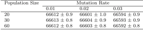
Table 6 Profit performance for base case (in RMU)±std. err. for three different population sizes and mutation rates.
Population Size Mutation Rate
0.01 0.02 0.03
20 66612±0.9 66601±1.0 66594±0.9
30 66613±0.8 66604±0.9 66593±0.9
60 66612±0.8 66603±0.8 66592±0.8
of all the demands to be scheduled, i.e., 225 in the industrial case study used here (the number of elements in Table 1). Specifically, each demand is given a unique ID number (from 1 to 225), and the chromosome is a permutation of these numbers. The ordering of the numbers on the chromosome determines the order by which the construction heuristic processes the respective demands (from first to last position) and thus influences the resulting schedule.
Originally, we initialised individuals randomly, but then realised that bet-ter solutions are produced if demands from a single year are grouped together on the chromosome. Unless stated otherwise, the results in this paper are thus based on runs where 50% of the population is initialised randomly, whereas the other 50% only randomise the sequence of demands from the same year, but maintain the sequence of years (i.e., all demands of a particular year appear in the permutation before the demands of later years). For fitness evaluation, the GA calls the construction heuristic described in Section 4.1 which builds a schedule by inserting demands iteratively in the order prescribed by the so-lution’s chromosome. The actual fitness is then the overall profit of the result-ing schedule, i.e., revenue minus storage, production, setup cost and backlog penalty. This objective function is defined mathematically in the Appendix. We did not spend much effort on tuning parameters to this problem, but ex-periments with different population sizes and mutation rates show that results are rather insensitive to the parameter settings (see Table 6). For the rest of the paper, we used a population size of 30, generational reproduction with elite of 6, and fitness proportional selection with stochastic universal sampling. For crossover, we used the Precedence Preserving Crossover (PPX) proposed by Bierwirth et al (1996) which ensures that if a demand i is before a demand
j in both individuals, this will also be true in the offspring. As the mutation operator we used shift mutation, which iterates through every element of the permutation and, with probabilitypm= 0.02, removes a demand and re-inserts it at a new random position. The algorithm is run for 1500 generations, and all results are based on averages over 50 runs.
5 Empirical evaluation
5.1 Comparison with mathematical programming
study has ample production capacity, which is due to modelling the option of outsourcing production at higher cost as additional facilities. To see how our algorithm would perform also in a more loaded scenario, we also tested variations of the case study where we increased the demand in each year by a factor of 2 or 3, and the results of these experiments are reported in Table 7 as well.
To judge the performance of our proposed algorithm, we compare it with a mixed integer linear programming (MILP) implementation as described by Lakhdar et al (2007) and replicated in the Appendix. We re-implemented the approach and compared the results of the GA with the results we obtained with our mathematical programming implementation. This ensures that the solutions are generated with exactly the same assumptions and data. However, there is one important difference that deserves discussion. The MILP model has variables that specify how much is produced for each facility, product and time period. It thus requires the problem to be broken down into discrete time periods, and it allows for at most one product to be produced in a particular facility and time period. The choice of the length of a time period is some-what arbitrary, but has huge implications. If the time period is chosen very large, then most demands would require only a fraction of a time period to be produced, the facility would be idle in the remaining part of the time period, leading to poor solutions. On the other hand, if the length of a time period is chosen to be rather short, because the number of batches to be produced is integer, often a fraction of the time period remains unused (e.g., if a time period is 5 days, and producing a batch takes 3 days, only one batch can be produced in each time period and 2 days in each time period remain unused -up to the point where a time period is too short for even one batch and there is no feasible solution). Furthermore, reducing the length of the time period increases the number of variables and constraints quite significantly, with cor-responding drastic implications on running time. After some experimenting, we concluded that the 90 day period used by Lakhdar et al (2007) indeed performs well, and all our results are based on this time granularity.
Time [years]
2005 2010 2015 2020
F
a
ci
li
ty
i10 i9 i8 i7 i6 i5 i4 i3 i2 i1
GA
- Pro
-
t: 66618 [RMU], CSL: 100.00%
P
ro
d
u
ct
0 5 10 15
Time [years]
2005 2010 2015 2020
F
a
ci
li
ty
i10 i9 i8 i7 i6 i5 i4 i3 i2 i1
MILP
- Pro
-
t: 66316 [RMU], CSL: 99.94%
P
ro
d
u
ct
0 5 10 15
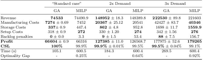
[image:16.595.88.395.120.366.2]Table 7 Profit, customer service level (CSL), and other characteristics for GA and MILP. For the GA, mean±std. err. are listed, whereas MILP is a deterministic method and was only run once. Best mean is highlighted inbold- where the difference is not significant both are highlighted. GA timing values are the average time elapsed for each of the 50 runs (i.e., the total runtime of 50 runs divided by 50).
“Standard case” 2x Demand 3x Demand
GA MILP GA MILP GA MILP
Revenue 74533 74490.9 148952±18.3 148389.8 222530±89.8 221603
Manufacturing Costs 7274±0.69 7452 20367±25.12 20541 42427±83.7 40346
Storage Costs 337±0.9 447.4 862±4.8 952.8 1698±11.7 1559.9
Setup Costs 318±0.9 272 330±1.20 274 342±1.56 276
Backlog penalties 0±0.0 3.3 9±1.5 53.4 88±7.5 156.7
Profit 66604±0.9 66316 127385±11.0 126568.7 177975±52.6 179265
CSL 100% 99.9% 99.9%±0.01% 99.5% 99.5%±0.04% 99.1%
Time (s) 105.1 600.5 184.3 600.4 269.5 600.4
Optimality Gap - 0.25% - 0.64% - 0.92%
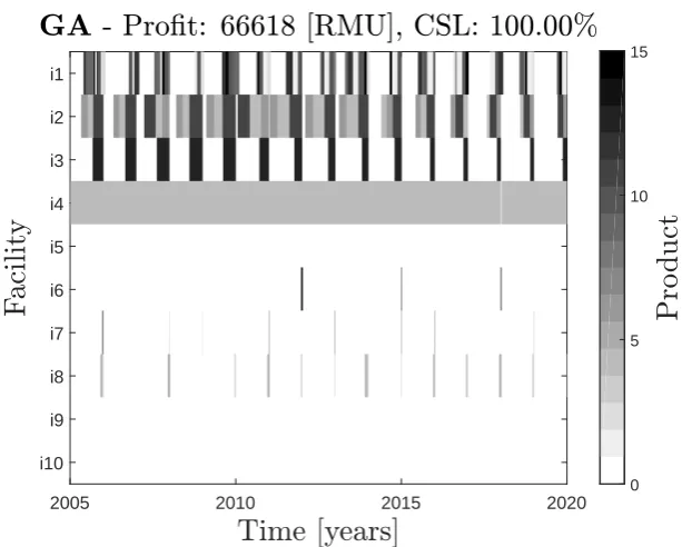
Results from the MILP model and the GA are compared in Table 7. As can be seen, in the standard case as taken from Lakhdar et al (2007), the GA solution has lower manufacturing costs, i.e., utilises better the low-cost facilities, and lower storage costs. It also manages to satisfy all the demand (customer service level of 100%), whereas the MILP model chooses to backlog some of the demand. This is because the GA tries to satisfy all the demand as first priority and only backlogs if there is no other feasible option. The MILP, however, has an explicit trade-off between backlog and other costs, and backlogs if the resulting solution has a higher profit. On the other hand, the setup costs of the GA solution are higher. Overall, the profit generated by the GA solution is consistently higher, and by more than the 0.25% optimality gap, i.e. the difference between the best solution found and the upper bound determined by the MILP solver. This is possible because MILP, due to its imposed time granularity, has an artificially restricted search space. It can switch less often between products, resulting in lower setup cost and higher storage cost. Also, it sometimes wastes part of a time period, which may mean the need to use occasionally more expensive facilities, resulting in higher manufacturing costs. These differences can be seen also by comparing the Gantt charts of the optimal solutions found by the MILP and the GA which are depicted in Figure 2. The Gantt chart of the MILP solution generally shows shorter campaigns (sequences of batches of the same product), and, especially visible on facility i4, small gaps between production in different time periods, simply because the time period (of 90 days) is not equivalent to a duration spanned by a multiple of batches for this product in this facility. The schedule optimised by the GA has longer un-interrupted idle time, which may be advantageous if a new product is introduced to the facility or if a third party is seeking to rent and use production capacity.
Table 8 Runtime of MILP until it reached an optimality gap of 0.25%, and runtime of GA to reach the same solution quality as was reached by MILP, for different problem sizes, depending on problem size.
15 years 23 years 30 years
Target (RMU) 66284 90236 111229
MILP Time (s) 200.86 824.134 1332.59
GA Time (s) 0.07 0.131 0.195
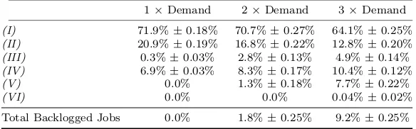
Table 9 Breakdown of how often each part of the heuristic is used in optimised solutions, mean±std. error. Also detailed is the percentage of separate jobs that are delivered late.
1×Demand 2×Demand 3×Demand
(I) 71.9%±0.18% 70.7%±0.27% 64.1%±0.25%
(II) 20.9%±0.19% 16.8%±0.22% 12.8%±0.20%
(III) 0.3%±0.03% 2.8%±0.13% 4.9%±0.14%
(IV) 6.9%±0.03% 8.3%±0.17% 10.4%±0.12%
(V) 0.0% 1.3%±0.18% 7.7%±0.22%
(VI) 0.0% 0.0% 0.04%±0.02%
Total Backlogged Jobs 0.0% 1.8%±0.25% 9.2%±0.25%
savings that can be achieved in terms of manufacturing cost and setup cost seem to outweigh this loss, and the overall profit of the MILP approach is higher in this scenario. Whether a slightly higher profit justifies a lower cus-tomer service level is a different issue. The GA’s construction heuristic, always tries to meet all the demand, even if this may lead to a possibly lower profit. Finally, we observe that the GA has still lower storage cost and higher setup cost, probably due to not being constrained by the coarse time periods.
Runtimes strongly depend on the implementation skills of the developer, the hardware used, and software tools used, and thus have to be handled with caution. Nonetheless, Table 7 also reports on the runtime of the two algo-rithms. For MILP, the stopping criterion was 600s, so the runtime remained the same, but the optimality gap increased as the problem became more dif-ficult by increasing the demand and thus utilisation level. The GA was run for a fixed number of generations. The computational time still increased with increasing the demand level. The reason is that an increasing demand raises the utilisation level and the construction heuristic is then less likely to be able to schedule a demand in steps (I) or (II), and thus more often has to look at the other alternatives for scheduling it. This will be explored further in the next subsection.
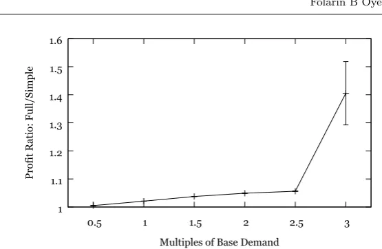
[image:18.595.95.387.207.298.2]1 1.1 1.2 1.3 1.4 1.5 1.6
0.5 1 1.5 2 2.5 3
Profit Ratio: Full/Simple
Multiples of Base Demand
Fig. 3 The ratio in profit of the full model compared to the simple model, optimized by the GA, shown for multiples of the base market demand as presented in the case study. The increasing ratio indicates the increasing benefit the full model will have in more complicated scheduling problems than the basic case study. Error bars represent the standard error.
solution. This profit value was then used as a target for the GA. The average time over the 50 runs that it took for the GA to match or beat those targets was recorded. The results of this experiment are shown in Table 8. As can be seen, the time required for the MILP and GA increases roughly linearly with problem size, however the factor by which runtime increases when moving from 15 to 30 years is 6.6 for MILP, but only 2.8 for the GA.
Overall, from these results, we conclude that the suggested GA approach is competitive with the MILP approach, but does not suffer from the intro-duction of artificial time periods and thus is sometimes able to find better solutions than MILP. The trend seems to be that the times for both optimisa-tion methods are going up linearly. However the increase of the GA approach is of a smaller factor than that of the MILP optimisations. This suggests that the relative performance of the GA is less susceptible to the detrimental impact of increasing the scale of the problem.
5.2 Algorithm components
In order to better understand the importance and robustness of the various components of our algorithm, we did some additional experiments.
[image:19.595.93.371.70.251.2]scenarios with higher demand, the percentage drops from 92.8% to 78.9%. This still constitutes the majority of cases, but clearly the other insertion alternatives of the heuristic become more important.
Figure 3 looks at the relevance of the alternatives (III)-(VI) in terms of their impact on profit. It shows the ratio of the obtained profit depending on whether the construction heuristic during the GA search was limited to looking at alternatives (I) + (II) (denoted as “Simple”), or all alternatives (“Full”). A profit ratio of 1 means that the two models obtain the same profit, while a greater profit ratio indicates that the full model is able to achieve higher profits than the simple model. It confirms that the more complicated cases with splitting, backlogging and moving previously scheduled demand are responsible for an increasing share of the profit as the overall demand is increased. Especially once the demand is increased to three times the original values, there seems to be a step change and the more complicated alternatives seem to become indispensable.
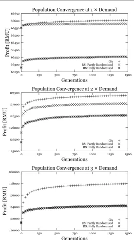
66250 66300 66350 66400 66450 66500 66550 66600 66650
0 250 500 750 1000 1250 1500
Profit [RMU]
Generations
Population Convergence at 1 × Demand
GA RS: Partly Randomised RS: Fully Randomised
125000 125500 126000 126500 127000 127500
0 250 500 750 1000 1250 1500
Profit [RMU]
Generations
Population Convergence at 2 × Demand
GA RS: Partly Randomised RS: Fully Randomised
170000 172000 174000 176000 178000 180000
0 250 500 750 1000 1250 1500
Profit [RMU]
Generations
Population Convergence at 3 × Demand
GA RS: Partly Randomised RS: Fully Randomised
[image:21.595.101.377.80.573.2]6 Conclusion
In this paper, we have considered the lot sizing and scheduling problem for a complex biopharmaceutical production scenario featuring multiple products, multiple facilities, and batch processing. For this challenging optimisation problem, we have proposed an GA based on an indirect permutation encoding that is decoded into a full schedule by a novel construction heuristic tailored to the problem at hand. A comparison with an MILP approach from the lit-erature showed that the GA is at least competitive, and often produces even better results than the MILP approach. The reason is that the MILP model artificially imposes a time granularity by dividing the time into discrete peri-ods that is not needed in the GA approach. This shows that although GAs are heuristic methods, they can sometimes outperform exact methods not only in terms of running time, but also because they are able to work with a model closer to reality.
In the future, we are considering various extensions of the proposed GA. First, in reality, demand is estimated and uncertain, so we would like to adapt our approach to stochastic and dynamic problems. This would also hopefully be a good juncture to investigate different instances of the problem solved in this work. Second, often in biopharmaceutical production, other objectives such as risk play a role, and an extension of our approach to the multi-objective case seems straightforward. Third, we plan to capture more realistic biophar-maceutical processes, e.g., by modelling multiple production stages. Fourth, the biopharmaceutical industry has seen a resurgence of interest in alternative ways to batch manufacturing, in particular continuous manufacturing, and so we would like to extend our algorithmic framework to also be applicable to this form of manufacturing. Fifth, from a theoretical perspective, it would be important to investigate the formal properties of the proposed GA to, for ex-ample, guarantee that the optimal schedule is indeed within reach of the search algorithm. Finally, one might explore also other optimisation methodologies to solve this problem such as constraint programming (Laborie, 2009) or hybrid approaches (Blum and Raidl, 2016).
Appendix
The appendix summarises the mathematical programme used in this paper and introduced by Lakhdar et al (2007).
Notation
Binary Variables
Yipt 1 if productpis produced over periodtat
facil-ityi; 0 otherwise
Zipt 1 if a new campaign of productpat facilityiis
started in periodt; 0 otherwise
Integer Variables
Bipt amount of productpproduced over periodt at
facilityi, batches
Continuous Variables
Ipt amount of productpstored over period t,
kilo-grams
Kipt amount of productpproduced over periodt at
facilityi, kilograms
P rof expected operating profit, RMU
Spt amount of product pwhich is sold over period
t, kilograms
Tipt production time for product pat time periodt
at facilityi
T ftotit total production time over periodtat facilityi
Wpt amount of productpwasted over periodt,
kilo-grams
∆pt amount of productpwhich is late over periodt,
kilograms
Parameters
Cp storage capacity of productp, kilograms
Dpt demand of productpat time periodt, kilograms
rip production rate of productpat facility i, batches per unit time
Ht available production time horizon over time periodt
Tmax
ip maximum production time for productp
Tipmin minimum production time for productp ydip yield conversion factor, kilograms per batch
αip lead time for production of first batch of productpat facility i
ζp life time of productp, number of time periodst
υp unit sales price for each kilogram of productp, RMU per kilogram
ηip unit cost for each batch produced of productpin facilityi, RMU per batch
ψp unit cost for each new campaign of productp, RMU
δp unit cost charged as penalty for each late kilogram of prod-uctp, RMU per kilogram
ρp unit cost for each stored kilogram of productp, RMU per kilogram
Production Constraints
Constraint (1) represents batch processing. The number of batches produced in facilityiof productpat time period t,Bipt, is determined by a continuous production rate,rip, production lead time,αip, and production timeTipt. The lead time allows for the duration of the first batch of a campaign plus the setup and cleaning time before the first batch commences. Incorporation of lead time is enforced by a binary variableZipt.
Bipt=Zipt+rip(Tipt−αipZipt) ∀i, p∈P Ii, t∈T Ii (1)
Constraint (2) converts the number of batches into kilograms produced us-ing a yield conversion factorydip which differs for each combination of facility and product. Lead time is only avoided in a facility if the same product is manufactured in the preceding period; this is covered in (3). Constraint (4) ensures that at most one productpis manufactured in any given facilityiper time periodt.
Kipt=Biptydip ∀i, p∈P Ii, t∈T Ii (2)
Zipt≥Yipt−Yip,t−1 ∀i, p∈P Ii, t∈T Ii (3)
X
p∈P Ii
Yipt≤1 ∀i, t∈T Ii (4)
Timing Constraints
Constraints (5) and (6) represent the appropriate minimum and maximum production time constraints. These are only active ifYipt is equal to 1, other-wise the production times are forced to 0.
TipminYipt≤Tipt ∀i, p∈P Ii, t∈T Ii (5)
Tipt≤min{Tipmax, Ht}Yipt ∀i, p∈P Ii, t∈T Ii (6)
Storage Constraints
The following constraints enforce an inventory balance for production and force total production to meet product demand. In (7), the amount of product
product storage capacity in (8); and total inventory at any point cannot exceed the global storage capacity in (9).
Ipt=Ip,t−1+
X
i
Kipt −Spt−Wpt ∀p∈P Ii, t∈T Ii (7)
0≤Ipt≤Cp ∀p, t (8)
0≤X
p
Ipt ≤CPtot ∀t (9)
The duration a product can be stored in inventory is limited by its shelf-life in (10).
Ipt≤
t+ζp X
θ=t+1
Spθ ∀p, t (10)
Backlog Constraints
A penalty is incurred for every time periodtthat a given amount of productp
is late. For a given productpat timet, the amount of product that is late,∆pt, is equal to the amount of undelivered product from the previous time period,
∆p,t−1, multiplied by a factor,πp(which allows for the backlog to decay), plus demand at timet,Dpt, less the sales at timet,Spt.
∆pt=πp∆p,t−1+Dpt−Spt ∀p, t (11)
Objective Function
The objective function is to maximise profit, which is the difference between total revenue (sales in kilogram times priceυp), and total operating costs which include the changeover cost atψp per setup, storage cost atρp per kilogram of product, late delivery penalties of δp per kilogram of product, and batch manufacturing cost atυipfor every product-facility combination. All costs and prices are in relative monetary units (RMU).
max Profit =X
p X
t∈T Ii
(υpSpt−ρpIpt−δp∆pt− X
i∈IPp
References
Almada-Lobo B, James RJ (2010) Neighbourhood search meta-heuristics for capacitated lot-sizing with sequence-dependent setups. International Jour-nal of Production Research 48(3):861–878
Almada-Lobo B, Klabjan D, Ant´onia carravilla M, Oliveira JF (2007) Sin-gle machine multi-product capacitated lot sizing with sequence-dependent setups. International Journal of Production Research 45(20):4873–4894 Almeder C (2010) A hybrid optimization approach for multi-level capacitated
lot-sizing problems. European Journal of Operational Research 200(2):599– 606
Bierwirth C, Mattfeld D (1999) Production scheduling and rescheduling with genetic algorithms. Evolutionary Computation 7(1):1–18
Bierwirth C, Mattfeld DC, Kopfer H (1996) On permutation representation for scheduling problems. In: Parallel Problem Solving from Nature, Springer, pp 310–318
Bitran GR, Yanasse HH (1982) Computational complexity of the capacitated lot size problem. Management Science 28(10):1174–1186
Blum C, Raidl GR (2016) Hybrid Metaheuristics: Powerful Tools for Opti-mization. Springer
Branke J, Mattfeld D (2005) Anticipation and flexibility in dynamic schedul-ing. International Journal of Production Research 43(15):3103–3129 Burke EK, Gendreau M, Hyde M, Kendall G, Ochoa G, ¨Ozcan E, Qu R (2013)
Hyper-heuristics: a survey of the state of the art. Journal of the Operational Research Society 64(12):1695–1724
Cheng R, Gen M, Tsujimura Y (1996) A tutorial survey of job-shop schedul-ing problems usschedul-ing genetic algorithms—i. Representation. Computers and Industrial Engineering 30(4):983–997
Copil K, W¨orbelauer M, Meyr H, Tempelmeier H (2017) Simultaneous lot-sizing and scheduling problems: a classification and review of models. OR Spectrum 39(1):1–64
Dangelmaier W, Kaganova E (2013) Robust solution approach to CLSP prob-lem with an uncertain demand. In: Robust Manufacturing Control, Springer, pp 455–467
DiMasi JA, Grabowski HG (2007) The cost of biopharmaceutical R&D: is biotech different? Managerial and Decision Economics 28(4-5):469–479 Drexl A, Kimms A (1997) Lot sizing and scheduling - survey and extensions.
European Journal of Operational Research 99:221–235
Farid SS (2007) Process economics of industrial monoclonal antibody manu-facture. Journal of Chromatography B 848(1):8–18
Gatica G, Papageorgiou L, Shah N (2003) Capacity Planning Under Uncer-tainty for the Pharmaceutical Industry. Chemical Engineering Research and Design 81(6):665–678
Goren HC, Tunali S, Jans R (2008) A review of applications of genetic algo-rithms in lot sizing. Journal of Intelligent Manufacturing 21(4):575–590 Ho JC, Chang YL, Solis AO (2006) Two modifications of the least cost per
period heuristic for dynamic lot-sizing. Journal of the Operational Research Society 57(8):1005–1013
James RJW, Almada-Lobo B (2011) Single and parallel machine capacitated lotsizing and scheduling: New iterative MIP-based neighborhood search heuristics. Computers and Operations Research 38(12):1816–1825
Jans R, Degraeve Z (2007) Meta-heuristics for dynamic lot sizing: A review and comparison of solution approaches. European Journal of Operational Research 177(3):1855–1875
Jans R, Degraeve Z (2008) Modeling industrial lot sizing problems: A review. International Journal of Production Research 46(6):1619–1643
Jin Y, Branke J (2005) Evolutionary optimization in uncertain evolutionary optimization in uncertain environments—a survey. IEEE Transactions on Evolutionary Computation 9(3):303–317
Karimi B, Fatemi Ghomi S, Wilson J (2003) The capacitated lot sizing prob-lem: a review of models and algorithms. Omega 31(5):365–378
Kimms A (1999) A genetic algorithm for multi-level, multi-machine lot sizing and scheduling. Computers and Operations Research 26(8):829–848 Laborie P (2009) IBM ILOG CP optimizer for detailed scheduling illustrated
on three problems. In: van Hoeve WJ, Hooker J (eds) International Confer-ence on Integration of AI and OR Techniques in Constraint Programming for Combinatorial Optimization Problems, Springer, LNCS, vol 5547, pp 148–162
Lakhdar K, Zhou Y, Savery J, Titchener-Hooker NJ, Papageorgiou LG (2005) Medium term planning of biopharmaceutical manufacture using mathemat-ical programming. Biotechnology Progress 21(5):1478–1489
Lakhdar K, Savery J, Papageorgiou LG, Farid SS (2007) Multiobjective long-term planning of biopharmaceutical manufacturing facilities. Biotechnology progress 23(6):1383–93
Levis AA, Papageorgiou LG (2004) A hierarchical solution approach for multi-site capacity planning under uncertainty in the pharmaceutical industry. Computers & Chemical Engineering 28(5):707–725
Luke S, Panait L, Balan G, Paus S, Skolicki Z, Kicinger R, Popovici E, Sul-livan K, Harrison J, Bassett J, Hubley R, Desai A, Chircop A, Comp-ton J, Haddon W, Donnelly S, Jamil B, Zelibor J, Kangas E, Abidi F, Mooers H, O’Beirne J, Talukder, Khaled Ahsan McDermott J (2014) ECJ: A Java-based Evolutionary Computation Research System. URL https://cs.gmu.edu/ eclab/projects/ecj/
Mehdizadeh E, Hajipour V, Mohammadizadeh MR (2016) A bi-objective multi-item capacitated lot-sizing model: Two Pareto-based meta-heuristic algorithms. International Journal of Management Science and Engineering Management 11(4):279–293
¨
Journal of Operational Research 110(3):525–547
Paul S, Mytelka D, Dunwiddie C, Persinger C, Munos B, Lindborg S, Schacht A (2010) How to improve r&d productivity: the pharmaceutical industry’s grand challenge. Nature Reviews Drug Discovery 9:203–214
Piperagkas GS, Konstantaras I, Skouri K, Parsopoulos KE (2012) Solving the stochastic dynamic lot-sizing problem through nature-inspired heuristics. Computers and Operations Research 39(7):1555–1565
Pitakaso R, Almeder C, Doerner KF, Hartl RF (2007) A MAX-MIN ant sys-tem for unconstrained multi-level lot-sizing problems. Computers and Op-erations Research 34(9):2533–2552
Ramya R, Rajendran C, Ziegler H (2016) Capacitated lot-sizing problem with production carry-over and set-up splitting: mathematical models. Interna-tional Journal of Production Research 54(8):2332–2344
Siganporia CC, Ghosh S, Daszkowski T, Papageorgiou LG, Farid SS (2014) Capacity planning for batch and perfusion bioprocesses across multiple bio-pharmaceutical facilities. Biotechnology Progress 30(3):594–606
Silver EA, Meal HC (1973) A heuristic for selecting lot size quantities for the case of a deterministic time-varying demand rate and discrete opportunities for replenishment. Production and inventory management 14(2):64–74 Wagner HM, Whitin TM (1958) Dynamic version of the economic lot size
model. Management Science 5(1):89–96
![Table 4 Manufacturing Costs of Facilities for Industrial Case Study [RMU/batch]](https://thumb-us.123doks.com/thumbv2/123dok_us/9442549.451506/7.595.74.411.508.607/table-manufacturing-costs-facilities-industrial-case-study-batch.webp)