An Efficient Direct Method to Solve the Three Dimensional Poisson’s Equation

(1)

An Efficient Direct Method to Solve the Three Dimensional

Poisson’s Equation

Alemayehu Shiferaw, Ramesh Chand Mittal

Department of Mathematics, Indian Institute of Technology, Roorkee, India E-mail: [email protected], [email protected]

Received August 24, 2011; revised October 11, 2011; accepted October 20, 2011

Abstract

In this work, the three dimensional Poisson’s equation in Cartesian coordinates with the Dirichlet’s boundary conditions in a cube is solved directly, by extending the method of Hockney. The Poisson equation is approximated by 19-points and 27-points fourth order finite difference approximation schemes and the resulting large algebraic system of linear equations is treated systematically in order to get a block tri-diagonal system. The efficiency of this method is tested for some Poisson’s equations with known analytical solutions and the numerical results obtained show that the method produces accurate results. It is shown that 19-point formula produces comparable results with 27-point formula, though computational efforts are more in 27-point formula.

Keywords: Poisson’s Equation, Finite Difference Method, Tri-Diagonal Matrix, Hockney’s Method, Thomas Algorithm

1. Introduction

Poisson’s equation in three dimensional Cartesian coordinates system plays an important role due to its wide range of application in areas like ideal fluid flow, heat conduction, elasticity, electrostatics, gravitation and other science fields especially in physics and engineering. For Dirichlet’s and mixed boundary conditions, the solution of Poisson’s equation exists and it is unique. Using some existing methods like variable separable or Green’s func- tion we can find the solutions of Poisson’s equation ana- lytically even though at times it is difficult and tedious from the point view of practical applications for some boundary conditions [1-4]. For further applications, it seems very plausible to treat numerically in order to obtain good and accurate solution of Poisson’s equation. The advantages of numerical treatment is to reduce com- plexities of the problem, secure more accurate results and use modern computers for further analysis [1,2,5].

If possible, direct methods are certainly preferable to iterative methods when several sets of equations with the same coefficients matrix but different right-hand sides have to be solved. It is well known that direct methods solve the system of equations in a known number of arithmetic operations, and errors in the solution arise entirely from rounding-off errors introduced during the

computation [1,5-7].

(2)

cients for the solution and those for the right-hand side. In this method the Fast Fourier Transform is used for the computation and its influence on the accuracy of the so-lution. Greengard and Lee [14] have developed a direct, adaptive solver for the Poisson equation which can achieve any prescribed order of accuracy. Their method is based on a domain decomposition approach using lo- cal spectral approximation, as well as potential theory and the fast multipole method.

To solve the three dimensional Poisson’s equations in Cartesian coordinate systems using finite difference approximations; for instance, Spotz and Carey [15] have developed an approximation using central difference scheme to obtain a 19-point stencil and a 27-point stencil with some modification on the right hand side terms; Braverman et al. [16] established an arbitrary order accuracy fast 3D Poisson Solver on a rectangular box and their method is based on the application of the discrete Fourier transform accompanied by a subtraction tech- nique which allows reducing the errors associated with the Gibbs phenomenon; Sutmann and Steffen [17] have developed compact approximation schemes for the La- place operator of fourth- and sixth-order based on Padé approximation of the Taylor expansion for the discre-tized Laplace operator; Jun Zhang [18] has developed a multigrid solution for Poisson’s equation and their finite difference approximation is based on uniform mesh size and they have solved the resulting system of linear equations by a residual or multigrid method.

The aim of this paper is to develop a fourth order finite difference approximation schemes and the resulting large algebraic system of linear equations is treated system- aticcally in order to get a block tri-diagonal system [19] and extend the Hockney’s method to solve the three dimensional Poisson’s equation on Cartesian coordinate systems. It is shown that the discussed method produces very good results. It is found that, in general, 27-points scheme produces better results than 19-points scheme but 19-point scheme also shows comparable results.

2. Finite Difference Approximation

Consider the Poisson equation





2 2 2

2

2 2 2 , ,

u u u

u f

x y z

  

    

   x y z D





on

and



, ,

ug x y z on C (1)

where and

is the boundary of







.



, , : 0 ,0 ,0

D x y z  x a  y b z c D

C

Let the mesh size along the X-direction and Y-direction be , and along the Z-direction be ( and

need not be equal ).

1

h h2 h1 h2

Let x be the central difference operator, and we

know that

 

2 2 4 1 2 2 2 1 2 2 4 1 2 2 2 1 2 2 4 2 2 2 2 1 1 1 12 1 1 12 1 1 12 x x y y z z u O h x h u O h y h u O h z h            _           _           _     

(2)

Using (2) in (1), we have

   

2 2

2 2 2 2

1 1

2

4 4

1 2 , , , ,

2 2 2 1 1 1 1 12 12 1 1 12 y x x y z

i j k i j k

z

h h

O h O h u f

h                _ _      _ _ _ _         _          (3)

where i1, 2,3, , , m j1, 2,3, , n and k1, 2,3, , p Letting 2 1 2 2 h r h

 , simplifying and neglecting the trun- cation error in (3), we get

2 2 2

2 1 , ,

2 2 2

1 1

12 12

1 1 1

12 12 12

1 1

12 12

1 1 1

12 12 12

1 1

12 12

x y z

i j k

x y z

y x z

x y z

z x y

h f r                  _  _      _ _ _        _ _  _  _        _  _          _  _  _           _  _         _{, ,}

2 2 2

1 1 1

12 12 12

i j k

x y z

u        _  _  _             (4)

2 2 2 2

1 ,

2 2 2 2 2

2 2 2

1 1 1

12 12 12

1 1 1 1

12 12 12 12

1 1

12 12

x y z i j k

x y z y x

z x y

(3)

















2 2 2 2

1

2 2 2 2 2 2 2 2 2

, ,

2 2 2 2 2 2 2 2 2

2 2 2 , , 1 1 12 1 1 144 1728 1 1 6 12 2 144

x y z

x y x z y z x y z i j k

x y z x y x z y z

x y z i j k h f r r r u                                    _    _          _  (5)

and this is a 19-point stencil scheme.

The Poisson’s Equation (1) now is approximated by its equivalent systems of linear equations either (6a) or (6b) and these equations now will be treated in order to form a block tri-diagonal matrix. We can find the eigenvalues and eigenvectors of these block tri-diagonal matrices easily.

Now we solve these two different systems of linear equations systematically.

On simplifying (5), Scheme 1

Considering all the terms of (5), we obtain

































2 2 2 2

1

2 2 2 2 2 2 2 2 2

, ,

, , , , 1 , , 1

1, , 1, , , 1, , 1,

1, 1, 1, 1, 1, 1, 1,

144 12

1

12

400 200 100 40

80 20

20 2

x y z

x y y z x z x y z i j k

i j k i j k i j k

i j k i j k i j k i j k

i j k i j k i j k i j

h

f

r u r u u

r u u u u

                          _ _ _        _              



  

















1,

1, , 1 1, , 1 1, , 1 1, , 1

, 1, 1 , 1, 1 , 1, 1 , 1, 1

1, 1, 1 1, 1, 1 1, 1, 1 1, 1, 1

1, 1, 1 1, 1, 1 1, 1, 1

8 10

2

k

i j k i j k i j k i j k

i j k i j k i j k i j k

i j k i j k i j k i j k

i j k i j k i j k i

r u u u u

u u u u

r u u u u

u u u u

                                                   

    1, 1, 1j k



(6a)

Taking first in the X-direction, next Y-direction and lastly Z-direction in (6a) and (6b), we get a large system of linear equations (the number of equations actually depends on the values of m, n and p); and this system of equations can be written in matrix form (for both schemes) as

AU   (7) where

R S S R S

S R S A

S R S S R                     

 (8)

it has p blocks and each block is of order mn mn

1 2

2 1 2

2 1

R R

R R R

R

R R R

R R                       ,

This is a 27-point stencil scheme. Scheme 2

By omitting the term



₂

  

₁₄₄



2 2 2

x y z

r   

 in the

left side and taking only the first and second terms in the right side of (5) and simplifying it, we get

































2 2 2 2

1 , ,

, , , , 1 , , 1

1, , 1, , , 1, , 1,

1, 1, 1, 1, 1, 1, 1, 1,

1, , 1 1, , 1 1, , 1 1, 1

12 1 12

32 16 8 4

6 2 2

1

x y z i j k

i j k i j k i j k

i j k i j k i j k i j k

i j k i j k i j k i j k

i j k i j k i j k i j

h f

r u r u u

r u u u u

u u u u

r u u u u

                         _ _ _                     



  



, 1

, 1, 1 , 1, 1 , 1, 1 , 1, 1

k

i j k i j k i j k i j k

u u u u



       

   

(6b)

1 2

2 1 2

2 1

S S

S S S

S

S S S

S S                       R m m

and have nS blocks and each block is of order

 where for theScheme 1

1

400 200 80 20

80 20 400 200 80 20

80 20 400 200 80 20 80 20 400 200

r r

r r r

(4)

r

r 2

80 20 20 2

20 2 80 20 20 2

20 2 80 20 20 2 20 2 80 20

r r

r r r

R

r r

 

 

 _ _ _ 

 

    

  

 

 _ _ _ 

 

 _ _ 

 



1

100 40 8 10

8 10 100 40 8 10

8 10 100 40 8 10 8 10 100 40

r r

r r r

S

r r r

r r

 

 

 _ _ _ 

 

    

  

 

 _ _ _ 

 

 _ _ 

 



2

8 10 2

2 8 10 2

2 8 10

r r

r r r

S

r r r

r r

 

 

 _ _ _ 

 

    

  

 

 _ _ _ 

 

 _ _ 

 



and forScheme 2

1

32 16 6 2

6 2 32 16 6 2

6 2 32 16

r r

r r r

R

r r

  

 

 _ _{ } _ 

 

     

  

 

 _ _{ } _ 

 

 _ _{ } 

 



2

6 2 2

2 6 2 2

2 6 2

r r

r R

r r



 

 _ 

 

  

  

 

 _ 

 

 _ 

 



1

8 4 1

1 8 4 1

1 8 4

r r

r r r

S

r r r

r r

 

 

 _ _ _ 

 

    

  

 

 _ _ _ 

 

 _ _ 

 



(5)

  2 1 1 1 1 r r S r r     _           _    

and for scheme 2

1

2

3 and ... p U U U u U                  1 2 3 ... p B B B b B                  where





11 21 1 12 22 2

1 2

k k k m k k k m

T

nk nk mnk

U u u u u u u

u u u

 

 

k



k

and b the known column vector Bk where





11 21 1 12 22 2

1 2

... ...

k k k m k k k m

T

nk nk mnk

B b b b b b b

b b b



 

such that each ijk represents known boundary values of

and values of b

u f .

3. Extended Hockney’s Method

Let i be an eigenvector of and 2 corresponding to the eigenvalues

q R R S1, 2, 1

, ,

i i i

S

   and i respec-

tively, and Q be the modal matrix



1, ,2 ,qm



m

3 of

the matrix and of order such that,

,

q q q

2 diag 1, 2, , ,3

T

n

Q S Q     

Note that the eigenvalues of and , for Scheme 1 are

1, 2, 1

R R S S2

π 400 200 2(80 20 ) cos

1 i i r r m       _ _    π

80 20 2(20 2 ) cos

1 i i r r m      _ _    π 100 40 2(8 10 ) cos

1 i i r r m      _ _    π

8 10 2(2 ) cos

1 i i r r m      _ _   

 



1 2,3, ,



diag , n

1 2 3



diag , , , ,

i    m

  

Here

π

2 cos 1

i i i

i m     _ _    and π 2 cos 1

i i i

i m     _ _    Let T

k k k

T

k k k

U V U V

B B B B

          k k (9) where





11 21 1 12 22 2

1 2

k k k m k k k m

T

nk nk mnk

V v v v v v

v v v

  

 

k

v

in order to find the solutions of Equation (1), we solve Equations (6a) and (6b).

Consider Equation (7) and using (8) we can write in it terms of the matrices R and S as

1 2 1

RU SU B

1 2 3

SU RU SU B₂

2 3 4

SU RU SU B₃ (10) 1

p p p

SU _ RU B

T

Pre multiplying (10) by  and using (9), we get

1 2

V V B1

   

1 2 3 2

V V V B

    

2 3 4

V V V B₃

      (11)

1

p p p

V _ V B

(6)

Each equation of (11) again can be written as

1 2

i ijv i ijv bij

   ₁

1 2 3 2

i ijv i ijv i ijv bij

   

2 3 4

i ijv i ijv i ijv bij

    ₃ (12)

( 1)

i ij pv i ijpv ijp

   b

For n an

For collect now from each equation

of s i.e. for , and get

1, 2,3, , i  m,

2,3, ,

k  p.



1, 2,3, ,

j  d

1, 

1, 2,3, ,

k  p

the first equation

(12), i1,j1

1 11(v k 1) 1v k v b

 _   _  (13a) (12) fo

11 1 11(k 1) 11k

Again collect the equations from r i2,j1

and get

2 21(k1) 2 21k 2 21(k1) 21k

Continuing in the same fashion and collecting t equations

v v v b

   

he at some point of , we get

(13b)

,

i j

( 1) ( 1)

i ij k i ijk i ij k ijk

And collecting the las quations (i.e. for i m,

v v v b

    t e

(13c)



jn), we get

( 1) ( 1)

m mn k m mnk m mn k mnk

(13a)-(13d) are tri-diag ce we so

v v v

   

All these set of Equations onal ones and hen lve for by using

algorithm, and with the help (9) ag we get a th

n’s by its fourth order pproximations scheme

e eigenvalues and eigenvectors of the

algorithm; for

ce ap oxim

irect

on r from

ro

es in which the analytical solutions of are known to us in order to test the

b (13d)

ijk

v ain

Thomas ll uijk and

is solves (6a) and (6b) as desired.

By doing this we generally reduce the number of computations and computational time.

4. Algorithm

1) Approximate the Poisson equatio finite difference a

2) Calculate th

block tri-diagonal matrices;

3) Find the modal matrix Q and ;

4) Pre multiply R S, and B_k by _T _{and get}

sys-tems of linear equations;

5) Solve the system by using Thomas 6) Calculate back ui j k, , .

Since we used finite differen pr ation to ap-proximate the Poisson equation’s and this method is d

in solution arises only e, it is sure that the erro the

unding off errors.By doing this we generally reduce the number of computations and computational time.

5. Numerical Results

A computational experiment is done on six selected

examples for both schem u

efficiency and adaptability of the proposed method. The computed solution is found for the entire interior grid points but results are reported with regard to the maximum absolute errors for corresponding choice of m n, ,p and the computed solutions are given in Tables 1-6.





0,

u









, ,1 1, , ,1, 1

u x y u y z u x z

   

u x y



, , 0



0

xy

u y z yz u x  z u x 

The analytical solution is and its results are shown in Table 2

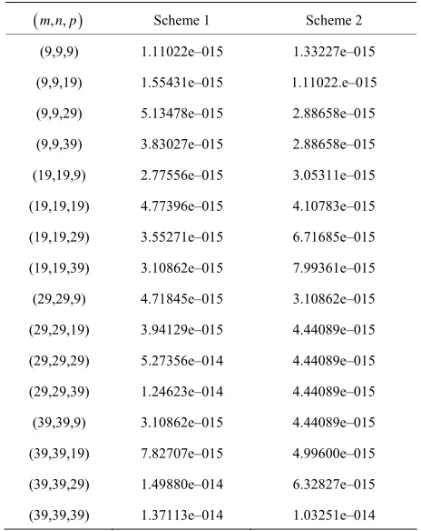
Example 3. Suppose with the

bo



, ,



u x y z xyz below.





2 ₂

u xy xz yz

   

undary conditions



0, ,





 









1, , 1 , ,1, 1

, ,1 1

u y z yz y z u z z z z

u x y xy x y



    

  

₁ 2 2_,



_{, ,1}



₁ 2

u x z  x z u x y  x y2

2 2

The analytical solution is 2_and its results are shown in Table 4

Example 5. Suppose z with the

bo



, ,



u x y z x y  below.

z

 

2 2_u _π _xy_si_n _π

 

undary conditions



0, ,





, 0,



u y z y

The analytical solution is and its results are shown in Table 5 belo

Example 6. Suppose

 

π uxysin z w.

  



2

2_u ₃_π _sin _π_x _sin

   πy

 

sin πz

(7)

[image:7.595.307.539.94.386.2]

Table 1. The maximum absolute error for Example 1.

e 1 Scheme 2

m n p, ,  Schem

(9,9,9) 1.99840e–015 1.55431e–015

(9,9,19) 5 2. 5

(

1.55431e–01 22045e–01

(9,9,29) 1.90958e–014 7.88258e–015 (9,9,39) 5.10703e–015 5.66214e–015

(19,19,9) 7.54952e–015 9.54792e–015 19,19,19) 1.55431e–015 1.19904e–014

(19,19,29) 6.43929e–015 2.15383e–014 (19,19,39) 7.21645e–015 234257e–014

(29,29,9) 1.69864e–014 1.11022e–014 (29,29,19) 9.43690e–015 4.66294e–015

(29,29,29) 1.63203e–014 6.66134e–015 (29,29,39) 3.96350e–014 8.43769e–015

(39,39,9) 6.43929e–015 5.77316e–015 (39,39,19) 2.33147e–014 2.88658e–015

[image:7.595.57.285.94.382.2]

(39,39,29) 4.46310e–014 1.62093e–014 (39,39,39) 3.29736e–014 1.39888e–014

Scheme 1 Scheme 2

m n p , , 

(9,9,9) 5.55112e–016 5.55112e–016

(9,9,19) 5.

(

7.77156e–016 55112e–016

(9,9,29) 2.83107e–015 1.30451e–015

(9,9,39) 1.72085e–015 1. 16573e–015

(19,19,9) 1.27676e–015 1.55431e–015

19,19,19) 2.33147e–015 1.99840e–015

(19,19,29) 1.38778e–015 3.38618e–015

(19,19,39) 1.33227e–015 3.99680e–015

(29,29,9) 2.44249e–015 1.52656e–015

(29,29,19) 1.77636e–015 2.02616e–015

(29,29,29) 2.80331e–015 1.67921e–015

(29,29,39) 6.16174e–015 2.08167e–015

(39,39,9) 1.24900e–015 1.66533e–015

(39,39,19) 3.69149e–015 1.88738e–015

(39,39,29) 7.54952e–015 3.05311e–015

(39,39,39) 6.59195e–015 4.49640e–015

m n p , ,  Scheme 1 Scheme 2 (9,9,9) 1.11022e–015 1.33227e–015

(9,9,19) 5 1. 5

(

1.55431e–01 11022.e–01

(9,9,29) 5.13478e–015 2.88658e–015 (9,9,39) 3.83027e–015 2.88658e–015

(19,19,9) 2.77556e–015 3.05311e–015 19,19,19) 4.77396e–015 4.10783e–015

(19,19,29) 3.55271e–015 6.71685e–015 (19,19,39) 3.10862e–015 7.99361e–015

(29,29,9) 4.71845e–015 3.10862e–015 (29,29,19) 3.94129e–015 4.44089e–015

(29,29,29) 5.27356e–014 4.44089e–015 (29,29,39) 1.24623e–014 4.44089e–015

(39,39,9) 3.10862e–015 4.44089e–015 (39,39,19) 7.82707e–015 4.99600e–015

(39,39,29) 1.49880e–014 6.32827e–015 (39,39,39) 1.37113e–014 1.03251e–014

[image:7.595.58.287.414.717.2]

e ma te error 4. Table 4. Th ximum absolu for Example

m n p, ,  Scheme 1 Scheme 2 (9,9,9) 2.55351e–015 1.77636e–015

(9,9,19) 2.

(

3.10862e–015 22045e–015

(9,9,29) 1.74305e–014 7.43849e–015

(9,9,39) 6.88338e–015 5.88418e–015

(19,19,9) 7.54952e–015 9.32587e–015

19,19,19) 1.44329e–014 1.28786e–015

(19,19,29) 6.99441e–015 2.14273e–014

(19,19,39) 7.77156e–015 2.28706e–014

(29,29,9) 1.48770e–014 9.99201e–015

(29,29,19) 9.32587e–015 8.43769e–015

(29,29,29) 1.58762e–014 8.88178e–015

(29,29,39) 3.67484e–014 1.02141e–014

(39,39,9) 7.32747e–015 7.43849e–015

(39,39,19) 2.17604e–014 7.10543e–015

(39,39,29) 4.39648e–014 1.78746e–014

[image:7.595.307.538.415.713.2]

(8)

m n p , ,  Scheme 1 Scheme 2

(9,9,9) 5.89952e–006 5.90013e–006

(9,9,19) 3.

(

3.67647e–007 67666e–007

(9,9,29) 7.25822e–008 7.25853e–008 (9,9,39) 2.29611e–008 2.2962e–008

(19,19,9) 5.92320e–006 5.9233e–006 19,19,19) 3.69122e–007 3.69124e–007

(19,19,29) 7.28734e–008 7.28737e–008 (19,19,39) 2.30532e–008 2.30533e–008

(29,29,9) 5.94508e–006 5.94513e–006 (29,29,19) 3.70486e–007 3.70487e–007

(29,29,29) 7.31427e–008 7.31428e–008 (29,29,39) 2.31384e–008 2.31384e–008

(39,39,9) 5.94513e–006 5.94515e–006 (39,39,19) 3.70489e–007 3.70489e–007

(39,39,29) 7.31432e–008 7.31433e–008 (39,39,39) 2.31386e–008 2.31386e–008

Tab e maximu rror fo

Scheme 1 Scheme 2 le 6. Th m absolute e r Example 6.

m n p , , 

(9,9,9) 4.07466e–005 9.56601e–005

(9,9,19) 3.

(

2.80105e–005 9912e–005

(9,9,29) 2.73312e–005 2.79092e–005

(9,9,39) 2.72169e–005 2.35847e–005

(19,19,9) 1.52747e–005 1.01614e–005

19,19,19) 2.53918e–006 5.93387e–006

(19,19,29) 1.85988e–006 3.47172e–006

(19,19,39) 1.74565e–006 2.48652e–006

(29,29,9) 1.3916e–005 3.32432e–006

(29,29,19) 1.18059e–006 1.88497e–006 (29,29,29) 5.01294e–007 1.17049e–006

(29,29,39) 3.87057e–007 7.96897e–007

(39,39,9) 1.36876e–005 7.87013e–006

(39,39,19) 9.52114e–007 6.34406e–007

(39,39,29) 2.72819e–007 5.30167e–007

(39,39,39) 1.58582e–007 3.70168e–007



 

1, ,y z

 

u x



, ,0,

, ,1

z u z

u x y

  



,1,



u x z



x y, ,0

 

u

0,

u y

0

The analytical solution is



, ,



sin

    

πx sin πy sin π

u x y z  z



an able 6 above.

This example VI was considered as a test problem in [7] and [18], and the results show that our meth is more eme the step siz

In this work, the three dimensional Poisson’s equation in systems is approximated by a fourth order finite difference approximation scheme. Here we

[1] L. Collatz, “The Numerical Treatment of Differential Equa- r Verlag, Berlin, 1960.

[2] M. K. Jain, “Numerical Solution of Differential Equa-

d its results are shown in T

od accurate than their methods and in their sch

e is the same for all dimensions but in our case Z-direction can have a different step length.

6. Conclusions

Cartesian coordinate

used to approximate the Poisson’s equation by a 27- points scheme and a 19-points scheme, and in doing this by the very nature of finite difference method for elliptic partial differential equations, it resulted in transforming the Poisson’s equation (1) in to a large number of algebraic systems of linear Equations (6a) or (6b) which forms a block tri-diagonal matrix in both schemes. These block tri-diagonal matrices are quite comfortable to find the eigenvalues and eigenvectors in order to extend Hockney’s method to three dimensions, and we have suc- cessfully reduced matrix A to a tri-diagonal one and by the help of Thomas Algorithm we solved the Poisson’s equation. The main advantage of this method is that we have used a direct method to solve the Poisson’s equation for which the error in the solution arises only from rounding off errors; because it’s a direct method the solution of (1) is sure to converge as we are always solving (1) by transforming it in to a diagonally dominant tri- diagonal system of linear equations; and it reduces the number of computations and computational time. It is found that this method produces very good results for fourth order approximations and tested on six examples. Actually it is shown that the discussed method, in general, for 27-points scheme produces better results than 19-points scheme but 19-point scheme has also shown comparable results.

Therefore, this method is suitable to find the solution of any three dimensional Poisson’s equation in Cartesian coordinates system.

7. References

(9)

Partial Differential

ew York, 1985.

duction to Numerical

Equa-0.321259

tions,” New Age International Ltd., New Delhi, 1984. [3] R. Haberman, “Elementary Applied

Equations with Fourier Series and Boundary Value Prob- lems,” Prentice-Hall Inc., Saddle River, 1987.

[4] T. Myint-U and L. Debnath, “Linear Partial Differential Equations for Scientists and Engineers,” Birkhauser, Bos- ton, 2007

[5] G. D. Smith, “Numerical Solutions of Partial Differential Equations: Finite Difference Methods,” Oxford Univer- sity Press, N

[6] G. H. Golub and C. F. van Loan, “Matrix Computations,” Johns Hopkins University Press, Baltimore, 1989. [7] J. Stoer and R. Bulirsch, “Intro

lysis,” Springer-Verlag, New York, 2002. [8] R. W. Hockney, “A Fast Direct Solution of Poisson

tion Using Fourier Analysis,” Journal of ACM, Vol. 12,

No. 1, 1965, pp. 95-113. doi:10.1145/32125

[9] W. W. Lin, “Lecture Notes of Matrix Computations,” Na- tional Tsing Hua University, Hsinchu, 2008.

[10] B. L. Buzbee, G. H. Golub and C. W. Nielson, “On Di- rect Methods for Solving Poisson’s Equations,” SIAM Journal on Numerical Analysis, Vol. 7, No. 4, 1970, pp.

627-656. doi:10.1137/0707049

[11] A. Averbuch, M. Israeli and L. Vozovoi, “A Fast Pois- son’s Solver of Arbitrary Order Accuracy in Rectangular regions,” SIAM Journal on Scientific Computing, Vol. 19,

No. 3, 1998, pp. 933-952.

doi:10.1137/S1064827595288589

[12] A. McKenney, L. Greengard and A. Mayo, “A Fast Pois- son Solver for Complex Geometries,” Journal of Compu-

tation Physics, Vol. 118, No. 2, 1996, pp. 348-355.

doi:10.1006/jcph.1995.1104

[13] G. Skolermo, “A Fourier Method for Numerical Solution

Direct Adaptive Poisson of Poisson’s Equation,” Mathematics of Computation, Vol.

29, No. 131, 1975, pp. 697-711. [14] L. Greengard and J. Y. Lee, “A

Solver of Arbitrary Order Accuracy,” Journal of Compu- tation Physics, Vol. 125, No. 2, 1996, pp. 415-424.

doi:10.1006/jcph.1996.0103

[15] W. F. Spotz and G. F. Carey, “A High-Order Compact

-2426(199603)12:2<235::AID-N

Formulation for the 3D Poisson Equation,” Numerical Methods for Partial Differential Equations, Vol. 12, No.

2, 1996, pp. 235-243.

doi:10.1002/(SICI)1098 UM6>3.0.CO;2-R

[16] E. Braverman, M. Israeli, A. Averbuch and L. Vozovoi, “A Fast 3D Poisson Solver of Arbitrary Order Accuracy,”

Journal of Computation Physics, Vol. 144, No. 1, 1998,

pp. 109-136. doi:10.1006/jcph.1998.6001

[17] G. Sutmann and B. Steffen, “High Order Compact Solvers for the Three-Dimensional Poisson Equation,” Journal of Computation and Applied Mathematics, Vol. 187, No. 2,

2006, pp. 142-170. doi:10.1016/j.cam.2005.03.041

[18] J. Zhang, “Fast and High Accuracy Multigrid Solution of the Three Dimensional Poisson Equation,” Journal of Computation Physics, Vol. 143, No. 2, 1998, pp. 449-

461. doi:10.1006/jcph.1998.5982

[19] M. A. Malcolm and J. Palmer, “A Fast Method for Solv- ing a Class of Tri-Diagonal Linear Systems,” Communi- cations of the ACM, Vol. 17, No. 1, 1974, pp. 14-17.