Trainer aircraft wing aerodynamic analysis considering turbulence at operational speed

TRAINER AIRCRAFT WING AERODYNAMIC ANALYSIS CONSIDERING TURBULENCE AT

*,

1

_{Research Scholar,}

2

_{Professor Institute of Aeronautical Engineering, Hyderabad}

ARTICLE INFO ABSTRACT

Light aircraft are being used widely for passenger and freight transport nowadays. In this paper aerodynamics of a trainer aircraft’s 3d wing with NACA 2412 aerofoil is presented. The lift and drag coefficient of the 3d wing at different angle’s of attack

plots of flow parameters like velocity, pressure and path lines are given. In this work kω sst Turbulence model is used to analyze the flow around the 3d wing of the trainer aircraft considering nominal wind t

considered taking symmetry in to account. Fuselage is not considered in this work since the objective of this work is to predict the performance of wing alone. Trainer

240km/hr is simulated to compute lift and drag coefficients of the wing at different angle of attacks.

Copyright©2016, Balaji and Dr. Dash. This is an open access article distributed under the Creative Commons Att use, distribution, and reproduction in any medium, provided the original work is properly cited.

INTRODUCTION

Small and light aircraft manufacturers are working on several development and research works for design and performance improvements of these small aircrafts for fuel economy and for reliable operations at varying weather conditions. A 3d wing of a trainer aircraft with NACA 2412 aerofoil profile is modelled to same scale and solved using CFD software to predict and tabulate the lift and drag coefficients at different angle of attacks. By this work the performance of a 3d wing of a trainer aircraft with a cruise speed of 240 km/hr is predicted for different angles of attack and it can be used for future research work in these area. When compared to a 2d infinite aerofoil analysis, 3d wing analysis will predict the drag and lift coefficients exactly taking in to account wing tip vortices downwash and varying wing thickness along the span. A flow analysis can be performed with different turbulence models an appropriate turbulence model has to be selected to predict the lift and drag coefficients. The computational fluid domain is modelled with optimum number of cells based on solution convergence. (Douvi, 2012) Douvi C. Eleni and others in their paper discussed about NACA 0012 aerofoil lift and drag prediction using three different turbulence models

*Corresponding author: Balaji, R.

Research Scholar, JNTUH Hyderabad.

ISSN: 0975-833X

Article History:

Received 20th _{May, 2016}

Received in revised form 08th _{June, 2016}

Accepted 17th _{July, 2016}

Published online 31st July,2016

Key words:

CFD, Trainer Aircraft wing, K-ω SST turbulence model, Lift, Drag, 3d wing.

Citation: Balaji, R. and Dr. Dash, P. K. 2016. “Trainer aircraft wing aerodynamic analysis considering

Journal of Current Research, 8, (07), 34959-34967.

RESEARCH ARTICLE

TRAINER AIRCRAFT WING AERODYNAMIC ANALYSIS CONSIDERING TURBULENCE AT

OPERATIONAL SPEED

*,1

_{Balaji, R. and}

_{Dr. Dash, P. K.}

Research Scholar, JNTUH Hyderabad

Professor Institute of Aeronautical Engineering, Hyderabad

ABSTRACT

Light aircraft are being used widely for passenger and freight transport nowadays. In this paper aerodynamics of a trainer aircraft’s 3d wing with NACA 2412 aerofoil is presented. The lift and drag coefficient of the 3d wing at different angle’s of attack using CFD software Fluent is analyzed and the plots of flow parameters like velocity, pressure and path lines are given. In this work kω sst Turbulence model is used to analyze the flow around the 3d wing of the trainer aircraft considering nominal wind turbulence conditions. For this simulation only one wing of aircraft without fuselage is considered taking symmetry in to account. Fuselage is not considered in this work since the objective of this work is to predict the performance of wing alone. Trainer

240km/hr is simulated to compute lift and drag coefficients of the wing at different angle of attacks.

is an open access article distributed under the Creative Commons Attribution License, which use, distribution, and reproduction in any medium, provided the original work is properly cited.

Small and light aircraft manufacturers are working on several works for design and performance improvements of these small aircrafts for fuel economy and for reliable operations at varying weather conditions. A 3d wing of a trainer aircraft with NACA 2412 aerofoil profile is modelled D software to predict and tabulate the lift and drag coefficients at different angle of attacks. By this work the performance of a 3d wing of a trainer aircraft with a cruise speed of 240 km/hr is predicted for sed for future research work in these area. When compared to a 2d infinite aerofoil analysis, 3d wing analysis will predict the drag and lift coefficients exactly taking in to account wing tip vortices downwash and varying wing thickness along the span. As fluid flow analysis can be performed with different turbulence models an appropriate turbulence model has to be selected to predict the lift and drag coefficients. The computational fluid domain is modelled with optimum number of cells based on Douvi C. Eleni and others in their paper discussed about NACA 0012 aerofoil lift and prediction using three different turbulence models namely

Spalart Allmaras, k ε Realizable and k

concluded stating k-ω SST model as the most appropriate turbulence model for lift and drag coefficient estimations of a 2d aerofoil. Like this various research work had been carried out comparing the accuracy and applicability of each of the turbulence model for different fluid flow analysis and it is recommended that kw-sst Turbulence model predicts aerofoil lift and drag coefficients accurately for nominal turbulence Conditions. Hence for this analysis

is used to predict the lift drag and other flow parameters of the 3dwing.

Turbulence model governing equation

Turbulent flows are characterized by fluctuating velocity. Since these fluctuations can be of small scale and high frequency, they are too computationally expensive to simulate directly with engineering calculations

instantaneous governing equations can be time

ensemble-averaged, or otherwise manipulated to remove the small scales, resulting in a modified set of equations that can be solved very easily with less computational time. This modified equation’s contain additional unknown variables, and turbulence models are needed to determine these variables in terms of known quantities.

International Journal of Current Research

Vol. 8, Issue, 07, pp.34959-34967, July, 2016

INTERNATIONAL

Trainer aircraft wing aerodynamic analysis considering turbulence at operational speed

TRAINER AIRCRAFT WING AERODYNAMIC ANALYSIS CONSIDERING TURBULENCE AT

Professor Institute of Aeronautical Engineering, Hyderabad

Light aircraft are being used widely for passenger and freight transport nowadays. In this paper aerodynamics of a trainer aircraft’s 3d wing with NACA 2412 aerofoil is presented. The lift and drag using CFD software Fluent is analyzed and the plots of flow parameters like velocity, pressure and path lines are given. In this work kω sst Turbulence model is used to analyze the flow around the 3d wing of the trainer aircraft considering urbulence conditions. For this simulation only one wing of aircraft without fuselage is considered taking symmetry in to account. Fuselage is not considered in this work since the objective of this work is to predict the performance of wing alone. Trainer aircrafts operational max speed of 240km/hr is simulated to compute lift and drag coefficients of the wing at different angle of attacks.

ribution License, which permits unrestricted

Allmaras, k ε Realizable and k-ω SST model. They ω SST model as the most appropriate turbulence model for lift and drag coefficient estimations of a 2d aerofoil. Like this various research work had been carried racy and applicability of each of the turbulence model for different fluid flow analysis and it is sst Turbulence model predicts aerofoil lift and drag coefficients accurately for nominal turbulence Conditions. Hence for this analysis kw-sst turbulence model is used to predict the lift drag and other flow parameters of the

ulence model governing equation

Turbulent flows are characterized by fluctuating velocity. Since these fluctuations can be of small scale and high frequency, they are too computationally expensive to simulate directly with engineering calculations. Instead, the instantaneous governing equations can be time-averaged, averaged, or otherwise manipulated to remove the a modified set of equations that can be solved very easily with less computational time. This modified equation’s contain additional unknown variables, and turbulence models are needed to determine these variables in

INTERNATIONAL JOURNAL OF CURRENT RESEARCH

Based on classical approach (Reynolds Average Navier Stokes Equation) we have below listed Turbulence models

a) Zero Equation model: Mixing length model b) One Equation model: Spalart Allmaras model c) Two Equation model: k-epsilon and k-omega model d) Seven Equation model: Reynolds Stress model

Based on Space-filtered equations we have LES (Large Eddy Simulation) model. Out of above listed Turbulence model Spalart Allmaras model, k-ε , k-ω and SST k-ω model are explained below.

Spalart Allmaras turbulence model (One Equation Model):

The Spalart-Allmaras model is a simple one-equation model that solves a transport equation for the kinematic turbulent viscosity. The Spalart-Allmaras model was designed specifically for aerospace applications involving wall-bounded flows and has been shown to give good results for boundary layers subjected to adverse pressure gradients. The Spalart-Allmaras model is effectively a low-Reynolds-number model, requiring the viscous affected region of the boundary layer to be properly resolved. However in some CFD software, the Spalart-Allmaras model has been implemented to use wall functions when the mesh resolution is not fine enough. However, the Spalart-Allmaras model is still relatively new, and no claim is made regarding its suitability to all types of complex engineering flows

In Spalart Allmaras model the transport equation for ν is given below

( ) + ( ) = + ( {( + ) } +

) ) + - - - (1)

where is the production of turbulent viscosity and is the destruction of turbulent viscosity that occurs in the near-wall region due to wall blocking and viscous damping. and are constants and is the molecular kinematic viscosity. is a user-defined source term.

The turbulent viscosity, μ , is computed from

μ =ρνf - - - (2)

Where the viscous damping function, f , is given by

f = χ

χ

Where χ≡ν

ν - - - (3)

The production term, Gν, is modeled as

Gν= C ρSν - - - (4)

where S ≡ S + ν

κ f - - - (5)

and f = 1 χ

χ

Where C and κ are constants, d is the distance from the wall, and S is a scalar measure of the deformation tensor and is based on the magnitude of the vorticity and it is given by

S ≡ 2Ω Ω - - - (6)

where Ω is the mean rate of rotation tensor and is defined by

Ω = ( )

The Turbulence destruction term is modelled as

Yν= C pf (

ν

) - - - (7)

Where

f = g(1 + C

g + C )

/

g = r + C (r r)

And r ≡ ν

κ

, , and are constants and is given by on (6).

Standard turbulencemodel

The standard k-ε model is based on modelling transport equations for the turbulence kinetic energy (k) and its dissipation rate (ε). In the derivation of the k-ε model, it was assumed that the flow is fully turbulent, and the effects of molecular viscosity are negligible. The standard k-ε model is therefore valid only for fully turbulent flows. The two transport equation for standard k-ε model are

(ρk) + (ρku ) = ((μ+μ

σ ) ) + G + G ρε

Y + S - - - (8)

(ρε) + (ρεu ) = ((μ+

μ

σε)

ε

) + Cε ε

(G +

C εG ) C ερ

ε

+ Sε - - - (9)

Where G represents the generation of turbulence kinetic energy due to the mean velocity gradients, G is the generation of turbulence kinetic energy due to buoyancy. Y represents the contribution of the fluctuating dilatation in compressible turbulence to the overall dissipation rate. C ε,C ε, and C ε are

constants. σ and σε are the turbulent Prandtl numbers for k

and ε, respectively. S and Sε are defined source terms.

The turbulent viscosity, , is computed by combining and as

where is a constant.

Standard turbulencemodel

The standard k ω model is an empirical model based on transport equations for the turbulence kinetic energy (k) and the specific dissipation rate (ω). The transport Equations for the Standard k ω model from which the turbulence kinetic energy k and the specific dissipation rate ω are obtained is given below

(pk) + (pku ) = (Γ ) + G Y + S

- - -- (11)

(pω) + (pωu ) = (Γω

ω

) + Gω Yω+ Sω

- - - (12)

In above equations, G represents the generation of turbulence kinetic energy due to mean velocity gradients. Gω represents

the generation of ω. Γ and Γω represent the effective

diffusivity of k and ω, respectively. Y and Yω represent the

dissipation of k and ω due to turbulence. S and Sω are user

defined source terms. This turbulence model is not presented here in detail as in this paper the flow over the aircraft wing is analyzed using SST kω model.

SST turbulencemodel

In this model when compared to standard k ω model the turbulent viscosity is modified to account for the transport of the principal turbulent shear stress. This feature gives the SST

k ω model an advantage in terms of performance over both the standard k ω model and the standard k ε model. In this model cross diffusion term is included in the ω equation and a blending function is considered to ensure that the model equations behave appropriately in both the near wall and far field zones. The transport equation for SST k ω model is given by

( ) + ( ) = ( ) + +

- - - (13)

( ) + ( ) = ( ) + + +

- - - (14)

where and are the effective diffusivity of and respectively. Y and Yω represent the dissipation of k and ω due

to turbulence and Dω represents the cross diffusion term. S

and Sω are user defined source terms. G represents the

generation of turbulence kinetic energy due to mean velocity gradients and Gω represents the generation of ω,

G = ρu u ( ) - - - (15)

Gω=

α

ν G - - - (16)

Coefficient α is α=α∞

α (

α / ω

/ ω) - - - (17)

where α∞ = F α∞, + (1 F )α∞, and

Re =ρ

μω

α =α∞(

α /

/ ) - - - (18)

Constants = 6, Rw = 2.95, = and

= 0.072

Also α∞, =

β_,

β_∞

κ

σω, β_∞

and α∞, =

β_,

β_∞

κ

σ_ω, β_∞

where constant κ = 0.41 and α∞ = 1 and β∞ = 0.09

Also β_, = 0.075 and β_, = 0.0828 - - - (19)

The effective diffusivities in SST k ω model is given by

Γ = μ+μ

σ and Γω= μ+ μ

σω - - - (20)

where σ and σω are the turbulent Prandtl numbers for k and ω

respectively.

The turbulent viscosity μ =ρ

ω (

α,

Ω

ω)

- - (21)

where Ω ≡ 2Ω Ω

σ =

/σ_, ( )/σ_, and σω= /σω, ( )/σω,

- - - (22)

Ω is the mean rate‐of‐rotation tensor and α is defined in (18).

The blending functions, F and F in (22) are

F = tanh (Φ ) and F = tanh (Φ ) - - - (23)

where Φ = min ( max ( √

. ω ,

μ

ρ ω),

ρ

σω, ω ) -

- - - (24)

and Φ = max (2 √

. ω ,

μ

ρ ω) - - - (25)

where y is the distance to the next surface and Dω is the

positive portion of the cross‐diffusion term

The dissipation of k and ωin SST k ω model is given by

Yω=ρβω - - - (27)

where β=β(1 β

β ζ F(M )) and

β = β (1 +ζ F(M )) - - - (28)

and β = F β_, + (1 F )β_,

β = β_∞( / ( / β)

( / β)

)

Compressibility function, F(M ) in (28) is

F(M ) = 0 M ≤ M

M M M > M

where M ≡ , M = 0. 25 and a = γRT ,

The constants σ , = 1.176, σω, = 2.0, _{σ ,} = 1.0, σω, = 1.168, ζ = 1. 5, Rβ= 8, β_∞= 0. 09

a = 0.31, β_, = 0.075, β_, = 0.0828, α =

The cross diffusion term Dω in (24) is given by

Dω= 2(1 F )ρσω, 1

ω

∂k ∂x

∂ω

∂x

Geometry and grid

For wing, NACA 2412 Aerofoil profile is used and the wing 2d geometry is shown in Figure 1.

Fig. 1. NACA 2412 Aerofoil section

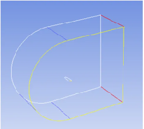
The fluid domain used to simulate the aerodynamic flow along with the 3d wing is shown in Figure 2.

Only one wing of the trainer aircraft is analyzed considering half symmetry. Fuselage is not considered for this analysis as only the performance of the wing is analyzed for different

angle of attacks and presented in this paper. Fluid domain is modelled accordingly to represent a large wind tunnel.

Fig.2. Fluid Domain with 3d wing

Grid element size is kept fine near to wing surface to capture Turbulent separated chaotic flow at high angle of attacks. In any CFD simulation before extracting the results the effect of mesh size on solution need to be investigated. In general accuracy of numerical solution will increase with number of grid cell or elements but it also will increase the computational time and additional memory requirements. An appropriate number of elements or cells can be determined by decreasing the mesh size such that it becomes finer and finer for each solution iteration and arriving at an appropriate size such that any further refinement will not have any significant change in solution values. For this 3d wing simulation solution convergence of lift coefficient at stall angle of attack is tested for different grid size and a optimum cell size is determined which lead to a converged solution. From the figure 3 it is clear that a grid size with 2959357 cells is found suitable for converged results.

Hence based on above convergence study, the computational domain which is used to simulate 3d wing at different angle of attacks is composed of 2955547 grid cells.

Fig. 4. Domain of 3d wing in CFD

Fig.5. Fine Grid size near to 3d wing (Loc ‘AA’)

In the domain the grid cells are clustered in such a way that boundary layer volume with fine grid size is created near to wing wall to capture turbulence separation and for accurate prediction of lift and drag coefficient. A moderate to coarse grid size is used in region away from wing surface in the fluid domain. CFD software Ansys Fluent 13 and workbench is used for flow simulation and grid generation of this 3d wing domain. In figure 4 domain grid with wing is shown. In figure 5 fine mesh near to 3d wing boundary layer is shown.

Properties and boundary

Conditions

Air at 273K and density of 1.2919 kg/m3 is considered for fluid domain assuming the aircraft will be operating at cold weather conditions. Boundary conditions like velocity inlet, walls without boundary layer and flow outlet with atmospheric pressure conditions are considered in the fluid domain as shown in figure 6 to represent conditions similar to wind tunnel.

Fig. 6. Fluid Domain Boundary conditions

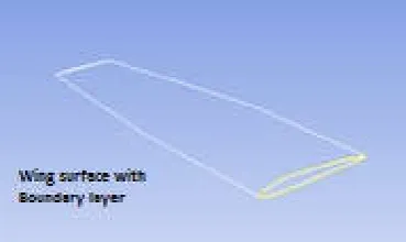
At 3d wing surface boundary condition of “No- Slip wall” is given to include boundary layer as shown in Figure 7.

Fig. 7. 3D Wing surface inside domain

Symmetric boundary condition is applied to wall which has the wing attached to it considering half symmetric analysis of full aircraft without fuselage. Velocity inlet condition of 63.9 m/s is considered at entry of domain to simulate the wing coefficients at 230 km/hr operating speed of aircraft. For this inlet conditions the Reynolds number of flow around the wing is approximately 4.9 million. Turbulence intensity of 0.5% is considered at flow inlet to simulate the lift and drag coefficients considering small amount of turbulence in the atmosphere at designated max and cruise altitude. Analysis was carried out for different angle of attack of 3d wing from -20o to +20o. k ω sst turbulence model is used for simulation of flow around the 3d wing, as several researches in similar kind of flows recommends kω sst model for accurate prediction of results. (Johansen, 1997) Johansen in his paper Prediction of Laminar/Turbulent Transition in Airfoil Flows discussed experimental results of fully turbulent and transitional turbulent flows around NACA 0012 aerofoil. Then (Douvi

et al., 2012) Douvi C .Eleni and other’s in their paper

“Evaluation of the turbulence models for the simulation of the flow over a NACA 0012 airfoil” compared experimental results of Johansen with Spalart Allmaras, k-ε and k-ω turbulence model and concluded k-ω turbulence model predicts lift and drag coefficients accurately than other two models. Based on this previous research work, kω sst turbulence model is used for flow simulation for this symmetric trainer aircraft NACA 2412 aerofoil 3d wing.

RESULTS AND DISCUSSION

Fig. 8. Lift coefficient of trainer aircraft wing for different angle of attack

Fig. 9. Drag coefficient of trainer aircraft wing for different angle of attack

Lift and Drag coefficient values computed using k

turbulence model for different angle of attack of the 3d trainer aircraft wing is listed below.

Fig. 10. Static Pressure plot at symmetric plane for 4 wing for different angle

Drag coefficient of trainer aircraft wing for different angle

Lift and Drag coefficient values computed using k-ω SST turbulence model for different angle of attack of the 3d trainer

Table 1. Lift and Drag coefficient values of trainer Aircraft wing for different angle of attack (Fluent results using k

Turbulence model)

S.No Angle of Attack

(In Degrees)

1 -20

2 -18

3 -15

4 -12

5 -4

6 0

7 4

8 12

9 15

10 18

11 20

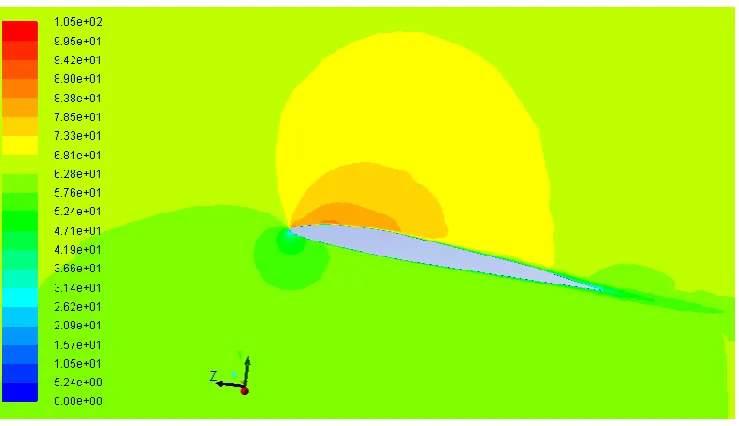
Figure 10, 11 and 12 shows the fluent cfd solution pressure contour around the wing at symmetric plane for 4

40 Angle of attack using k-ω sst turbulence model.

from Figure 10 and 11 that static pressure at lower surface of wing for 40 and 150 AOA is higher than the pressure at upper surface of wing due to which it creates lift force in upward direction. At negative AOA static pressure will be higher at top surface of the wing when compared to lower surface of wing as seen in Figure 12 which will push aircraft wing downwards.

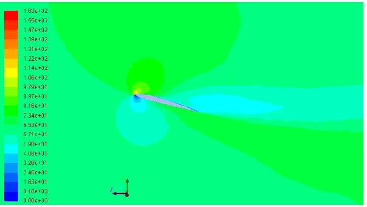
Also Velocity contour is shown for 4

figure 13, 14 and 15. It is seen from plot that from 4

AOA stagnation point will move forward from trailing edge towards leading edge. A stagnation point in a flow field is a point where local velocity is zero. It is noticed from figure 13 and figure 14 at positive AOA velocity at upper surface of wing is higher than at the lower surface which creates pressure difference between top and bottom surface and hence positive lift. It is also seen from figure

upper surface at 150 AOA is higher than that of velocity at 4 AOA.

Static Pressure plot at symmetric plane for 40 AOA with k-ω sst Turbulence model

Lift and Drag coefficient values of trainer Aircraft wing for different angle of attack (Fluent results using k-ω SST

Turbulence model)

k-ω SST Turbulence Model

Cl Cd

-0.624 0.275

-0.676 0.237

-0.727 0.188

-0.651 0.131

-0.185 0.013

0.109 0.010

0.392 0.022

0.948 0.110

1.17 0.174

1.33 0.271

0.915 0.345

Figure 10, 11 and 12 shows the fluent cfd solution pressure contour around the wing at symmetric plane for 40, 150 and

-ω sst turbulence model. It is seen from Figure 10 and 11 that static pressure at lower surface of AOA is higher than the pressure at upper e of wing due to which it creates lift force in upward direction. At negative AOA static pressure will be higher at top surface of the wing when compared to lower surface of 12 which will push aircraft wing

ty contour is shown for 40, 150 and -40 AOA in figure 13, 14 and 15. It is seen from plot that from 40 to 150 AOA stagnation point will move forward from trailing edge towards leading edge. A stagnation point in a flow field is a is zero. It is noticed from figure 13 and figure 14 at positive AOA velocity at upper surface of wing is higher than at the lower surface which creates pressure difference between top and bottom surface and hence positive lift. It is also seen from figure 13 and figure 14, velocity at AOA is higher than that of velocity at 40

Fig. 11. Static Pressure plot at symmetric plane for 150 AOA with k-ω sst Turbulence model

Fig. 12. Static Pressure plot at symmetric plane for 40 AOA with k-ω sst Turbulence model

Conclusion

In this paper lift and drag coefficient’s of a trainer aircraft wing obtained by CFD analysis is shown and listed out for different angle of attacks. K-ω SST Turbulence model which is widely used for external flows is used for CFD simulation of the 3D trainer aircraft wing. Properties of air at high altitude operating conditions and the cruise speed of trainer aircraft is considered for simulating the lift and drag coefficient at different angle of attack. In order to get accurate lift and drag coefficient of the said 3D aircraft wing, solution convergence study is done and a suitable grid size is selected before simulating the wing model for different angle of attack. It is observed from the results that lift coefficient increases with increase of AOA until 180 AOA after that it decreases. Static pressure plot and velocity plot at symmetric plan of wing is shown for different AOA. The experimental results of 2D NACA 2412 aerofoil wing is not compared with the trainer

aircraft wing lift and drag coefficient discussed in this paper as the effects of 3D wing swept back angle and the cord thickness variation along the span is not taken in to account in 2D infinite aerofoil results already available in literature. Experimental wind tunnel analysis can be carried out to find out the performance of wing at even higher AOA or higher levels of turbulence where software simulations cannot predict exact flow characteristics without known experimentally determined variable values.

REFERENCES

Bruhn, E. F. “ Analysis and Design of flight vehicle structures ” Tri-state offset company 1993 edition

Douvi C. Eleni, Tsavalos I. Athanasios and Margaris P. Dionissios “Evaluationof the turbulence models for the simulation of the flow over a National Advisory Committee for Aeronautics (NACA) 0012 airfoil”,

Fig. 14. Velocity plot at symmetric plane for 150 AOA with k-ω sst Turbulence model

published in Journal of Mechanical Engineering Research vol. 4(3), March 2012.

DR. Hermann Schlichting. “Boundary Layer Theory ” McGraw Hill Book company – seventh edition

Johansen, J. 1997. Prediction of Laminar/Turbulent Transition in Airfoil Flows. Riso National Laboratory, Roskilde, Denmark.

Justin Petrilli, Ryan Paul, Ashok Gopalarathnam and Neal T. Frink “A CFD Database for Airfoils and Wings at Post-Stall Angles of Attack” published in AIAA Journal. Ostowari, C. and Naik, D. 1984. “Post Stall Studies of

Untwisted Varying Aspect Ratio Blades with an NACA

4415 Airfoil Section—Part 1,” Wind Engineering, Vol. 8, No. 3.

Ryan Babigian and Shigeo Hayashibara “Computational study of the Vortex Wake Generated by a Three-Dimensional Wing with Dihedral, Taper and Sweep”, published in AIAA Applied Aerodynamics conference, 2009.

Vance Dippold, III,” Investigation of Wall Function and Turbulence Model Performance within the Wind Code”, published in AIAA Aerospace Sciences Meeting January 2005.