Particle Swarm Optimization for Identifying Rainfall Runoff Relationships

Particle Swarm Optimization for Identifying

Rainfall-Runoff Relationships

Chien-Ming Chou

Department of Design for Sustainable Environment, Ming Dao University, Changhua, Chinese Taipei Email:[email protected]

Received January 2, 2012; revised February 7, 2012; accepted March 4,2012

ABSTRACT

Rainfall-runoff processes can be considered a single input-output system where the observed rainfall and runoff are inputs and outputs, respectively. Conventional models of these processes cannot simultaneously identify unknown structures of the system and estimate unknown parameters. This study applied a combinational optimization and Parti- cle Swarm Optimization (PSO) for simultaneous identification of system structure and parameters of the rainfall-runoff relationship. Subsystems in proposed model are modeled using combinations of classic models. Classic models are used to transform the system structure identification problem into a combinational optimization and can be selected from those typically used in the hydrological field. A PSO is then applied to select the optimized subsystem model with the best data fit. The parameters are estimated simultaneously. The proposed model is tested in a case study of daily rain- fall-runoff for the upstream Kee-Lung River. Comparison of the proposed method with simple linear model (SLM) shows that, in both calibration and validation, the PSO simulates the time of peak arrival more accurately compared to the SLM. Analytical results also confirm that the PSO accurately identifies the system structure and parameters of the rainfall-runoff relationship, which are a useful reference for water resource planning and application.

Keywords: Rainfall-Runoff; System Identification; Particle Swarm Optimization; Classic Models; Simple Linear Model

1. Introduction

The rainfall-runoff process in a river basin can be con- ceptualized as a single input-output system. When mod- eling such a system, the goal is to use historic data for predicting further runoff by analyzing the input-output relationship based on observed input-output data, i.e., system identification. The “black-box” approach empha- sizes system functions rather than system characteristics or natural laws governing the system. The system re- sponse function analyzes the black-box relationships between inputs and outputs, i.e., the system characteris- tics or natural laws governing system operation. The system response function also varies according to system characteristics or according to natural laws. In black-box models, the task is describing or approximating the sys- tem response function.

The identifications and applications of hydrological black-box models have been thoroughly investigated. Cheng et al. [1] presented an automatic calibration methodology, which consists of water balance parameter and runoff routing parameter calibration, for Xinanjiang model. Their results showed that the hybrid methodology of genetic algorithms (GAs) and the fuzzy optimal model

(FOM) is not only capable of exploiting more the impor- tant characteristics of floods but also efficient and robust. Chau et al. [2] employed the GA-based artificial neural network (ANN-GA) and the adaptive-network-based fuzzy inference system (ANFIS) for flood forecasting in a channel reach of the Yangtze River in China. They found that the ANFIS model is optimal and the perform- ance of the ANN-GA model is also good.

passes the standard GA. Thus, their proposed approach was feasible and effective in optimal operations of com- plex reservoir systems.

Wang et al. [5] examined ARMA models, ANNs ap- proaches, adaptive neural-based fuzzy inference system (ANFIS) techniques, genetic programming (GP) models and SVM method using the long-term observations of monthly river discharges. They found that the best per- formance can be obtained by ANFIS, GP and SVM, in terms of different evaluation the training and validation phases. Wu et al. [6] proposed a crisp distributed support vectors regression (CDSVR) model for monthly stream- flow prediction in comparison with four other models: ARMA, K-nearest neighbors (KNN), ANNs, and crisp distributed ANNs (CDANNs). Their results showed that models fed by preprocessed data perform better than models fed by original data, and CDSVR outperform other models except for at a 6-month-ahead horizon for Danjiangkou. They also found that the performance of CDSVR deteriorated with the increase of the forecast horizon.

Hydrological models such as simple linear model (SLM) are suitable for hydrological system identification because they can simply and conventionally estimate total runoff from total rainfall. However, conventional models for performing the above system identification are limited because they cannot simultaneously identify the unknown structure of the system and estimate un- known parameters. Wang et al. [7] developed a new method of using Particle Swarm Optimization (PSO) algorithm for system identification. Its novel feature is the use of classic models to transform the system struc- ture identification problem into a combinational problem. A PSO algorithm is then used to identify system structure and parameters. This study applies the concept developed by Wang et al. [7] to model the rainfall-runoff relation- ship.

Kennedy and Eberhart [8] originally developed the PSO algorithm for a simplified simulation of animal so- cial behaviors. The PSO, which is a population-based and self-adaptive search optimization technique, is now widely used to solve discrete and continuous optimiza- tion problems. Recently, PSO has been employed exten- sively in hydrological forecasting and water resources management. Chau [9] developed a PSO model for training perceptions in ANNs. Applications of PSO pre- dicting water levels show that the technique is an effect- tive alternative algorithm for training ANNs.

Gill et al. [10] introduced PSO, a relatively new global optimization tool that has already proven effective and efficient in various fields. Although PSO initially had a single-objective function, the approach has been ex- tended to deal with multiple objectives in a form called multiobjective PSO (MOPSO). Tests of this approach for

parameter estimation of a well-known 13-parameter con- ceptual rainfall-runoff model of Sacramento soil mois- ture show very encouraging modeling results. Chau [11] developed and applied a split-step PSO model to train multi-layer perceptions for forecasting real-time water levels. This paradigm combines the advantages of the global search capability of PSO algorithm in the first step with fast local convergence of Levenberg-Marquardt algorithm in the second step. Performance comparisons show that its speed and accuracy are better than those of the benchmarking backward propagation algorithm and the standard PSO algorithm.

Luo and Yuan [12] used PSO to optimize an integrated water system by combining water usage processes and water treatment operations into a single network such that the total cost of fresh water and wastewater treat- ment is florally minimized. Zhang et al. [13] tested five global optimization algorithms (GAs, shuffled complex evolution, PSO, differential evolution, and artificial im- mune system) for automatic parameter calibration in a complex hydrologic model of four watersheds con- structed using Soil and Water Assessment Tool (SWAT). The results show that GA outperform the other four algo- rithms when more than 2000 models are analyzed while PSO obtains better parameter solutions when fewer than 2000 models are run. The PSO algorithm is preferable when computation time is limited whereas GA is prefer- able when substantial computational resources are avail- able. When applying both GA and PSO for optimizing SWAT parameters, the population size should be small.

In a SVM developed by Wang et al. [14] for forecast- ing annual reservoir inflow, PSO is used for parameter optimization. For the data set used in that study, the SVM model outperformed the ANN models in terms of forecasting performance. Gaur et al. [15] applied Ana- lytic Element Method (AEM) in a PSO-based simula- tion-optimization model of groundwater management problems. The AEM-PSO model proved efficient for optimizing the location and discharge of pumping wells. The penalty function approach was also effective when using PSO to solve groundwater hydraulic management problems.

neous identification of the system structure and parame- ters. The rest of this paper is organized as follows. First, the concept of system identification and the SLM struc- tures are described. The PSO algorithm and its imple- mentation procedure are then defined. Next the efficacy of the proposed method is demonstrated in a case study of a small Taiwan watershed. Finally, analytical results are discussed, and conclusions are given.

2. System Identification

2.1. The Description of System Identification

A system can be identified from observed input and out- put data to obtain the equivalent system. The purpose of system identification is to understand variation in the system so that the identified results can be applied to solving practical problems. The system identification in this study is the method that selects the combination of the subsystem model that best fits the sample data from many subsystems and estimates their parameters. Classic models are used to transform the system structure identi- fication problem into a combinational optimization prob- lem. The system model consists of subsystem models that are the combination of classic models. Classic mod- els can be selected from models typically used in the hydrological field. The principles of selecting classic models are general, classic and includable [7].

Consider a static system with multiple inputs and sin- gle output. Suppose that y is the output of an observable system affected by m input, i.e., x1, x2,···, xm. The n groups of observed data can be described as follows [7]:





, 1, 2, ,

ji

x i  n

 

  



Q t H I t

1 2

, , , i i i

y x x (1)

where xji is the j-th input data of group i, yi is the output data of group i, i = 1, 2,···, n; j = 1, 2,···, m.

Suppose that the observed data include various possi- ble subsystem models that are combinations of classic models. Classic models can be selected from the models that usually appear in the hydrological field. Now con- sider the case where single variable xj affects the output of system by the form of f(xj). The f(xj) is then defined as a classic model with a single variable [7]. Let N be the total number of classic models with a single variable. The output, which is affected by various input data, can be expressed as [7]

 

1 1

N m

i k

k j

y f

 





2.2. The Simple Linear Model

The simple and conventional method used to estimate the system response function from rainfall-runoff data is the SLM [16]. The SLM is compared with the proposed

method in this study.

Let I(t) and Q(t) represent total rainfall and total runoff of a watershed, respectively, and let H(t) represent the system response function. The rainfall-runoff process is assumed to be a linear, time-invariant, and single input- output system. The function of the SLM system can be represented by a linear convolution equation as follows [16]:

  



_

 

  



1

1

L

i

Q k H i I k i



(3)

where τis an integral variable.

Equation (3) can be applied in discrete form as follows [16]:





 

  

  

1

1

L

i

Q k H i I k i e k







1 1 1

n n L L n

(4)

where L is the memory length of a watershed, I(k – i + 1) is the average rainfall at time k – i + 1, Q(k) is the total runoff at time k, H(i) is a system response function.

Equation (5) reveals data error or incomplete assump- tions about linearity [16]:

(5)

where e(k) is a random error term.

Equation (5) can be expressed using matrix equations as follows [16]:

     

Q I H E

 

 



 



1

2

n

T T

i

T T T T T

J e i



    

  



(6)

where n is the total length of hydrological data, and L is the memory length of a system response function.

The system response function H can be identified by Least Squares (LS) method. The essential principle of LS is to minimize the sum of squares of the differences be- tween the observed and estimated values. The objective function is defined as follows [16]:

H E E Q IH Q IH

Q Q H I Q H I IH

(7)

The system response function can be derived by mini- mizing the objective function, i.e., min



 



1

ˆ T  T

as shown below [16].

   



H _I I_{ }I Q_ (8)

3. Particle Swarm Optimization

sonably good solution.

3.1. Underlying Theory of PSO

In PSO, several particles (M particles) are denoted as the potential solution flying in the problem search space to locate their optimum positions. Each particle is repre- sented by a vector in multidimensional space D. Assume the position vector and velocity vector of particle i are Xi = (xi1, xi2,···, xid) and Vi =(vi1, vi2,···, vid), respectively. Set pi = (pi1, pi2,···, pid), i.e., pbest, as the current optimal posi- tion searched by each particle, and set gbest as the current optimal position searched by all particles of the group. For each generation, the updated equations of particle velocity and position in dimension d

are as follows [17]:













1 1

1 1

1

k i d i d k i d

nd p x x

 

 

1 1

k k k

i d i d

2 2

k k

i d i d

g d

v wv c ra c rand p

 

  (9)

i d

x _x _v 

k

v

k

(10)

where w is the inertia weight coefficient, c1 and c2 are

acceleration coefficients, rand1 and rand2 are random

numbers in the interval [0,1], and i = 1, 2,···, M. The ia is the component of fly velocity vector of particle i in dimension d for generation k. The xid is the component of position vector of particle i in dimension d for genera- tion k. The pid is the component of the current optimal position vector pbestisearched by particle i in dimension d. The pgd is the component of the current optimal position vector gbestsearched by all particles of the group in di- mension d.

3.2. Algorithm Procedure

The procedure for performing the PSO algorithm is as follows [18].

1) Randomly generate both the position and velocity of the particle in the initial swarm for D-dimensional space.

2) Evaluate the fitness value of the particle, which is usually defined as

 

 

2

f 



y0(t) are the estimated and observed output, respectively.

3) Compare the fitness value of the particle with that of the previous optimal value, and modify the new velo- city of the particle according to the best positions of the particle (pbest) and swarm (gbest).

4) Compare the fitness of the particle and swarm. If the best fitness of the particle is superior to that of the swarm, modify the memory of the best fitness (gbest) value for the swarm. At the same time, every particle should modify the velocity of the particle in the next generation.

5) Determine the new velocities and positions of the particles for the next generation according to Equations

(9) and (10).

6) Stop the search when the termination condition is satisfied; otherwise, return to step 2). The algorithm usu-ally stops when the generation reaches the maximum.

4. Application and Analysis

4.1. The Proposed Method

Consider the three classic models for the relationship between rainfall input x and runoff output y, which is an example of a typical relationship in a hydrological system:



y ax

 2

y b x

 3

y cx

 

 

1 1 1 1

8 8 8

2 3

1 1 1

1, 2, ,

N m

i k ji k ji

k j k j

j ji j ji j ji

j j j

y f x f x

a x b x c x i n

   

  

 

   











(11)

(12)

(13)

where a, b and c are constant coefficients. The input used when testing the proposed PSO method is the daily rain- fall for the current day and the previous 7 days. The choice of the particular set of parameters is based on the memory length of a watershed. In addition, more pa- rameters are included because of carrying out the com- binational optimization. The daily runoff of current day is selected as output. To compare the proposed PSO with the SLM, the memory length of the watershed L is 8 days. Assume these eight inputs affect the output of sys-tem by the form f(xj). The n output can then be described as:

(14)

Equation (14), which includes both linear and nonlin- ear terms, is similar to the Volterra model typically used to identify a nonlinear system. Linear models yield fairly good results, so the effect of nonlinearity in modeling is assumed to be relatively small. Hence, Lattermann [19] considered that adding only a second term to the linear hydrological model is adequate. This investigation adopts sufficient three terms to the modeling of the nonlinear rainfall-runoff process. The coefficients of Equation (14) cannot be conveniently estimated by LS since the input matrix is singular when solving Equation (8). Some of the diagonal elements of the upper triangular matrix U of the lower and upper (LU) factorization approach zero. In this study, the PSO is applied to estimate the coefficients of Equation (14). The analytic results are compared with the results obtained using SLM.

4.2. Study Basin

   

 

The CE quantifiesthe goodness of fit between the esti- mated hydrograph and the observed hydrograph. A better fit is indicated by a CE that is closer to unity.

runoff processes using the Wu-Tu watershed, which located in northern Taiwan. The watershed upstream area is 203 km2 (Figure 1). The mean annual precipitation in this watershed is 2500 mm. Due to the topography of this watershed, the runoff pathlines are short and steep, and rainfall is nonuniform in both time and space. Large floods develop quickly in the middle-to-downstream reaches of this watershed, leading to severe damage. The daily rainfall and runoff data for 1966-1994 were collected. The data for 1966-1980 were used to calibrate the proposed model, while data for 1981-1994 were used to verify the performance of the proposed method. Each year is regarded as a single event (i.e., duration is 365 days) in calibration or validation. Daily rainfall data are average values obtained from the Jui-Fang, Huo-Shao- Liao and Wu-Tu weather station using the kriging me- thod. The daily runoff data are obtained from the Wu-Tu hydrological station.

2) Error of Total Volume (EV)

4.3. Comparison of Model Performances

1) Coefficient of efficiency, CE, is defined as:

2

2

ˆ

q i q i

q i q



 

 



 

 

 

q i

 

q i

1

1

1 n i

n i

CE 



 





where denotes the discharge of the simulated hy- drograph for time period i (m3/s), is the discharge of the observed hydrograph for time period i (m3/s), q

   

 

represents the average discharge of the observed hydro- graph for time period i (m3/s) and n is number of data.

1

1

ˆ

n

i n

i

q i q i EV

q i



 

 

 











 

q i

 

denotes the discharge of the simulated hy- drograph for time period i (m3/s), is the discharge of the observed hydrograph for time period i (m3/s). The

EV specifies the mean error between the estimated hy- drograph and the observed hydrograph. When the value of EV is positive, the mean estimated discharge exceeds the observed discharge, and vice versa. A better fit is represented by a smaller absolute value of EV.

3) The error of peak discharge, EQp (%), is defined as:

ˆ

% P P 100%

P

p

q q EQ

q



 

ˆ

(17)

where qP

P P

P T T

ET  ˆ 

denotes the peak discharge of the simulated hydrograph (m3/s) and qp is the peak discharge of the observed hydrograph (m3/s). When the EQp is positive, the estimated peak discharge exceeds the observed peak discharge. When EQp is negative, the estimated peak discharge is smaller than the observed peak discharge. A better fit is indicated by a smaller absolute value of EQp.

4) The error of the time for peak to arrive, ETp, is de- fined as:

(18)

ˆ P where T

 

H

ˆ i

b cˆ_i

denotes the time for the simulated hydro-graph peak to arrive (days) and Tp represents the time required for the observed hydrograph peak to arrive (days). When ETp is negative, the estimated peak dis-charge precedes the observed peak disdis-charge. When ETp is positive, the estimated peak discharge follows the ob-served peak discharge. A better fit is represented by a smaller absolute value of ETp.

5. Results and Discussion

The results obtained using SLM are denoted as the SLM. The results obtained using PSO in Equation (14) are de- noted as the PSO. For the proposed PSO method, the total number of particle swarms, the maximum number of generations, inertia weight coefficient w, and accelera- tion coefficients c1 and c2 are 36, 100, 0.5, 2.0 and 2.0,

respectively.

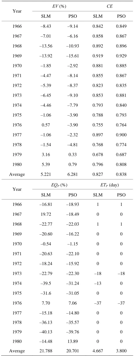
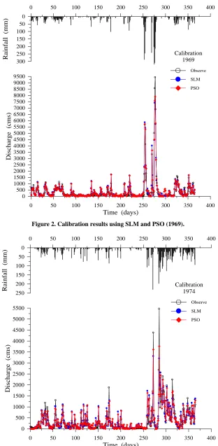
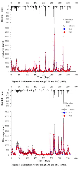
Table 1 shows the calibration results for the SLM and the PSO. Figures 2-5 display four representative cali- bration results. Calibration results show that the average absolute value of EV is slightly worse in the PSO (6.281%) than in the SLM (5.221%). Based on the aver- age value of the CE criterion, the PSO (0.838) outper- forms the SLM (0.827). The CE of the PSO also outper- forms that of the SLM for each year. Based on the EQP criterion, the average of the absolute value of the PSO (20.701%) is slightly better than that of the SLM (21.788%). Based on the ETP criterion, the average ab- solute value of the PSO (3.800 days) is better than that of SLM (4.667 days). Especially in the case of year 1974 (Figure 3), the ETP of SLM is –13 days; however, the

ETP of PSO is 0 days. The PSO obtains a more accurate simulation of the peak values compared to the SLM.

Table 2 presents the average value of the estimated coefficients of response function, i.e., , and the average value of the estimated coefficients of Equation (14), i.e., , and , obtained from the 15 cali- brated years. The average value of the estimated coeffi- cients can be used for performance evaluations of the SLM and PSO. The average of the estimated coefficients provides not only validation data for the proposed ap- proach, but also average system characteristics.

ˆ_i

a

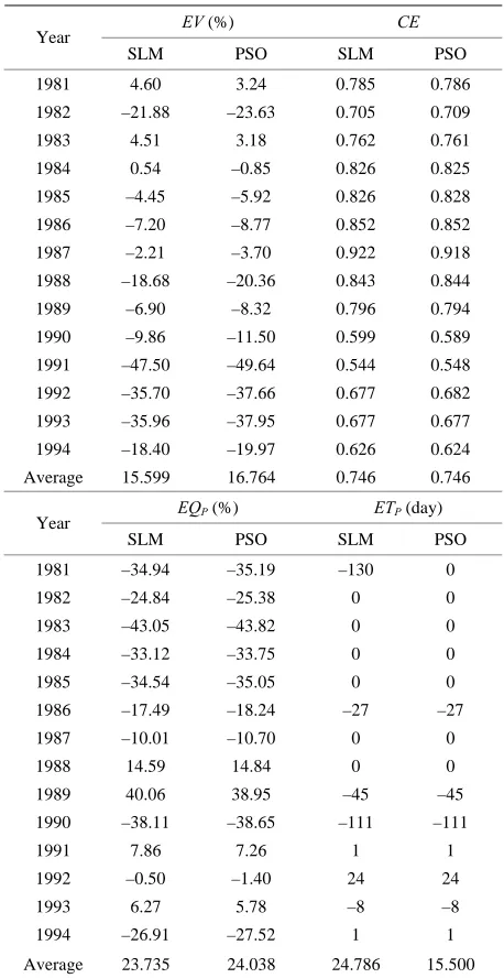
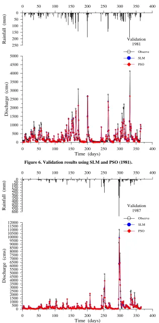
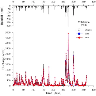
Table 3 shows the validation results when using SLM and PSO. Figures 6-9 display four representative vali- dation results. Validation results demonstrate that the average absolute value of EV of the PSO (16.764%) is slightly worse than that of the SLM (15.599%). Based on the CE criterion, the PSO performs comparably to the SLM. Based on the EQP criterion, the average of the ab- solute value of the PSO (24.038%) is slightly worse than that of the SLM (23.735%). Based on the ETP criterion, the average of the absolute value of the PSO (15.500 days) is better than that of SLM (24.786 days). Espe-

Table 1. Calibration results using SLM and PSO.

EV (%) CE

Year

SLM PSO SLM PSO

1966 –8.43 –9.14 0.842 0.849

1967 –7.01 –6.16 0.858 0.867

1968 –13.56 –10.93 0.892 0.896

1969 –13.92 –15.61 0.919 0.929

1970 –1.85 –2.92 0.881 0.885

1971 –4.47 –8.14 0.855 0.867

1972 –5.39 –8.37 0.823 0.835

1973 –6.45 –9.10 0.853 0.881

1974 –4.46 –7.79 0.793 0.840

1975 –1.06 –3.90 0.788 0.793

1976 0.57 –3.90 0.755 0.764

1977 –1.06 –2.32 0.897 0.900

1978 –1.54 –4.81 0.768 0.774

1979 3.16 0.33 0.678 0.687

1980 5.39 0.79 0.796 0.808

Average 5.221 6.281 0.827 0.838

EQP(%) ETP (day)

Year

SLM PSO SLM PSO

1966 –16.81 –18.93 1 1

1967 19.72 –18.49 0 0

1968 –22.77 –22.03 1 1

1969 –20.60 –16.22 0 0

1970 –0.54 –1.15 0 0

1971 –20.63 –22.10 0 0

1972 –18.24 –15.92 0 0

1973 –22.79 –22.30 –18 –18

1974 –39.5 –31.24 –13 0

1975 –31.6 –31.05 0 0

1976 7.70 7.06 –37 –37

1977 –15.18 –14.80 0 0

1978 –36.13 –35.57 0 0

1979 –40.13 –39.76 0 0

1980 –14.48 13.89 0 0

Average 21.788 20.701 4.667 3.800

Note: The columns for EV, EQP and ETP all contain negative values, and

0 50 100 150 200 250 300

Time (days)

350 400 0

500 1000 1500 2000 2500 3000 3500 4000 4500 5000 5500 6000 6500 7000 7500 8000 8500 9000 9500

Discharge

(cms)

0 50 100 150 200 250 300 350 400

0 50 100 150 200 250 300

Rai

n

fall

(mm)

Calibration 1969

Observe SLM PSO

Figure 2. Calibration results using SLM and PSO (1969).

0 50 100 150 200 250 300

Time (days)

350 400 0

500 1000 1500 2000 2500 3000 3500 4000 4500 5000 5500

Disch

a

rge (cms)

0 50 100 150 200 250 300 350 400

0

50

100

150

200

250

Rainfall

(mm)

Calibration 1974

Observe SLM PSO

0 50 100 150 200 250 300

Time (days)

350 400 0

500 1000 1500 2000 2500 3000 3500 4000 4500 5000

Disch

a

rge (cms)

0 50 100 150 200 250 300 350 400

0

50

100

150

200

250

Rainfall

(mm)

Calibration 1977

Observe SLM PSO

Figure 4. Calibration results using SLM and PSO (1977).

0 50 100 150 200 250 300

T

350 400

ime (days)

0 500 1000 1500 2000 2500 3000 3500 4000 4500

Discharge (cms)

0 50 100 150 200 250 300 350 400

0 50 100 150 200 250 300

Rai

n

fall

(mm

)

Calibration 1980

Observe SLM PSO

i i cˆi

Table 2. The average estimated coefficients, obtained from the 15 calibrated events.

cially in the case of year 1981 (Figure 6), the ETP of SLM is –130 days; however, the ETP of PSO is 0 days. The PSO can simulate the time of peak arrival more ac- curately compared to the SLM.

i _Hˆ aˆ bˆi

1 0.059619 0.057535 0.005992 –0.001940

2 0.233782 0.232144 –0.000360 –0.000630

3 0.046193 0.045697 0.005371 –0.002490

4 0.030542 0.030349 0.001085 0.001375

5 0.011485 0.012033 –0.000960 –0.002530

6 0.010943 0.009812 0.002254 0.000576

7 0.012044 0.010661 0.007537 0.000463

8 0.007258 0.003676 –0.001550 0.001933

The above results can be summarized as follows. In the case of calibration results, the PSO outperforms the SLM in all criteria except EV. In terms of CE criterion in particular, the PSO outperforms the SLM in each year. These calibration results imply that the proposed PSO is suitable for identifying the rainfall-runoff relationship. In the case of validation results, the CE of the PSO is the same as that of the SLM. The PSO is slightly worse than the SLM based on the EV and EQP criteria. However, the PSO clearly outperforms the SLM based on the ETP cri- terion. In both the calibration and validation results, the PSO can simulate the time of peak arrival more accu- rately compared to the SLM. This finding apparently shows that the PSO, which includes both linear and nonlinear terms, simulates the time of peak arrival more accurately compared to the SLM, which includes only linear terms.

Table 3. Validation results using SLM and PSO.

EV (%) CE

Year

SLM PSO SLM PSO

1981 4.60 3.24 0.785 0.786

1982 –21.88 –23.63 0.705 0.709

1983 4.51 3.18 0.762 0.761

1984 0.54 –0.85 0.826 0.825

1985 –4.45 –5.92 0.826 0.828

1986 –7.20 –8.77 0.852 0.852

1987 –2.21 –3.70 0.922 0.918

1988 –18.68 –20.36 0.843 0.844

1989 –6.90 –8.32 0.796 0.794

1990 –9.86 –11.50 0.599 0.589

1991 –47.50 –49.64 0.544 0.548

1992 –35.70 –37.66 0.677 0.682

1993 –35.96 –37.95 0.677 0.677

1994 –18.40 –19.97 0.626 0.624

Average 15.599 16.764 0.746 0.746

EQP(%) ETP(day)

Year

SLM PSO SLM PSO

1981 –34.94 –35.19 –130 0

1982 –24.84 –25.38 0 0

1983 –43.05 –43.82 0 0

1984 –33.12 –33.75 0 0

1985 –34.54 –35.05 0 0

1986 –17.49 –18.24 –27 –27

1987 –10.01 –10.70 0 0

1988 14.59 14.84 0 0

1989 40.06 38.95 –45 –45

1990 –38.11 –38.65 –111 –111

1991 7.86 7.26 1 1

1992 –0.50 –1.40 24 24

1993 6.27 5.78 –8 –8

1994 –26.91 –27.52 1 1

Average 23.735 24.038 24.786 15.500

6. Conclusions

In this work, performance in identifying rainfall-runoff relationships was compared between PSO and conven- tional SLM. The calibration results for PSO are better than those of the SLM in all criteria except EV. Specifi- cally, based on the CE criterion, the PSO outperforms the SLM in each year. The validation results for PSO are slightly worse than those for the SLM based on the EV and EQP criteria. The CE of the PSO is the same as that of the SLM. The PSO clearly outperforms the SLM based on the ETP criterion. The above results show that the proposed PSO is more suitable for modeling rain- fall-runoff relationships compared to SLM.

The estimated time of peak arrival is an essential cal- culation. Both the calibration and validation results con- firm that the PSO can simulate the time of peak arrival more accurately compared to the SLM. The main reason is that the PSO includes both linear and nonlinear terms whereas the SLM uses only linear terms.

This study applied PSO for identifying rainfall-runoff relationships. The PSO, which is a global random opti- mization algorithm, can simultaneously identify system structure and parameters. The daily rainfall-runoff data for the upstream Kee-Lung River are chosen to verify the appropriateness of the proposed model. Analytical results demonstrate that PSO effectively identifies the system structure and parameters of the rainfall-runoff relation- ship, which is an essential consideration in water re- source planning and application.

The inertia weight coefficient and acceleration coeffi- ients, which are used to adjust the velocities and posi-

Note: The columns for EV, EQPand ETPall contain negative values, and

0 50 100 150 200 250 300

Time (days)

350 400 0

500 1000 1500 2000 2500 3000 3500 4000 4500 5000

Di

sc

ha

rge

(cms

)

0 50 100 150 200 250 300 350 400

0

50

100

150

200

250

Rai

n

fall

(m

m)

Validation 1981

Observe SLM PSO

Figure 6. Validation results using SLM and PSO (1981).

0 50 100 150 200 250 300

Time (days)

350 400 0

500 1000 1500 2000 2500 3000 3500 4000 4500 5000 5500 6000 6500 7000 7500 8000 8500 9000 9500 10000 10500 11000 11500 12000

Di

sch

a

rg

e

(

cms)

0 50 100 150 200 250 300 350 400

0 50 100 150 200 250 300 350 400 450 500 550 600

R

a

in

fall

(mm)

Validation 1987

Observe SLM PSO

0 50 100 150 200 250 300

Time (days)

350 400 0

500 1000 1500 2000 2500 3000 3500 4000 4500 5000

Discharge (cm

s)

0 50 100 150 200 250 300 350 400

0 50 100 150 200 250 300

Ra

infa

ll

(mm)

Validation 1988

Observe SLM PSO

Figure 8. Validation results using SLM and PSO (1988).

0 50 100 150 200 250 300

Time (days)

350 400

0 500 1000 1500 2000 2500 3000

Dis

c

h

a

rge

(cms)

0 50 100 150 200 250 300 350 400

0

50

100

150

200

R

a

infal

l (m

m)

Validation 1992

Observe SLM PSO

tions of all the particles within each generation, play im- portant roles in PSO. In this study, inertia weight coeffi- cient w, and acceleration coefficients c1 and c2 are typi-

cally set to 0.5, 2.0 and 2.0, respectively. Much attention should be focused on how to determine their values. In practice, different improved method may be tried in the future regarding the main search procedure of the origin- nal PSO which is robust.

7. Acknowledgements

The author would like to thank the National Science Council, Taiwan for financially supporting this research under Contract No. NSC 100-2221-E-451-010.

REFERENCES

[1] C. T. Cheng, C. P. Ou and K. W. Chau, “Combining a Fuzzy Optimal Model with a Genetic Algorithm to Solve Multiobjective Rainfall-Runoff Model Calibration,” Jour- nal of Hydrology, Vol. 268, No. 1-4, 2002, pp. 72-86. doi:10.1016/S0022-1694(02)00122-1

[2] K. W. Chau, C. L. Wu and Y. S. Li, “Comparison of Several Flood Forecasting Models in Yangtze River,”

Journal of Hydrologic Engineering, Vol. 10, No. 6, 2005, pp. 485-491.

doi:10.1061/(ASCE)1084-0699(2005)10:6(485)

[3] J. Y. Lin, C. T. Cheng and K. W. Chau, “Using Support Vector Machines for Long-Term Discharge Prediction,”

Hydrological Sciences Journal, Vol. 51, No. 4, 2006, pp. 599-612. doi:10.1623/hysj.51.4.599

[4] C. T. Cheng, W. C. Wang, D. M. Xu and K. W. Chau, “Optimizing Hydropower Reservoir Operation Using Hybrid Genetic Algorithm and Chaos,” Water Resources

Management, Vol. 22, No. 7, 2008, pp. 895-909. doi:10.1007/s11269-007-9200-1

[5] W. C. Wang, K. W. Chau, C. T. Cheng and L. Qiu, “A Comparison of Performance of Several Artificial Intelli-gence Methods for Forecasting Monthly Discharge Time Series,” Journal of Hydrology, Vol. 374, No. 3-4, 2009, pp. 294-306. doi:10.1016/j.jhydrol.2009.06.019

[6] C. L. Wu, K. W. Chau and Y. S. Li, “Predicting Monthly Streamflow Using Data-Driven Models Coupled with Data-Preprocessing Techniques,” Water Resources

Re-search, 45, W08432, 2009, 23 Pages. doi:10.1029/2007WR006737

[7] F. Wang, K. Xing and X. Xu, “A System Identification Method Using Particle Swarm Optimization,” Journal of Xi’an Jiaotong University, Vol. 43, No. 2, 2009, pp. 116- 120 (in Chinese).

[8] J. Kennedy and R. C. Eberhart, “Particle Swarm Optimi- zation,” Proceedings of IEEE International Conference

on Neural Networks, Perth, Vol. 4, 1995, pp. 1942-1948. doi:10.1109/ICNN.1995.488968

[9] K. W. Chau, “Particle Swarm Optimization Training Al-gorithm for ANNs in Stage Prediction of Shing Mun River,” Journal of Hydrology, Vol. 329, No. 3-4, 2006, pp. 363-367. doi:10.1016/j.jhydrol.2006.02.025

[10] M. K. Gill, Y. H. Kaheil, A. Khalil, M. McKee and L. Bastidas, “Multiobjective Particle Swarm Optimization for Parameter Estimation in Hydrology,” Water Re- sources Research, Vol. 42, W07417, 2006, 14 Pages.

doi:10.1029/2005WR004528

[11] K. W. Chau, “A Split-Step Particle Swarm Optimization Algorithm in River Stage Forecasting,” Journal of Hydro-

logy, Vol. 346, No. 3-4, 2007, pp. 131-135.

[12] Y. Luo and X. G. Yuan, “Global Optimization for the Synthesis of Integrated Water Systems with Particle Swarm Optimization Algorithm,” Chinese Journal of Che- mical Engineering, Vol. 16, No. 1, 2008, pp. 11-15. doi:10.1016/S1004-9541(08)60027-0

[13] X. S. Zhang, R. Srinivasan, K. G. Zhao and M. V. Liew, “Evaluation of Global Optimization Algorithms for Para- meter Calibration of a Computationally Intensive Hydro-logic Model,” Hydrological Processes, Vol. 23, No. 3, 2008, pp. 430-441. doi:10.1002/hyp.7152

[14] W. C. Wang, X. T. Nie and L. Qiu, “Support Vector Machine with Particle Swarm Optimization for Reservoir Annual Inflow Forecasting,” Proceedings of International Conference on Artificial Intelligence and Computation Intelligence (AICI), Sanya, 2010, pp. 184-188.

doi:10.1109/AICI.2010.45

[15] S. Gaur, B. R. Chahar and D. Graillot, “Analytic Ele- ments Method and Particle Swarm Optimization Based Simulation—Optimization Model for Groundwater Man-agement,” Journal of Hydrology, Vol. 402, No. 3-4, 2011, pp. 217-227. doi:10.1016/j.jhydrol.2011.03.016

[16] Y. X. Wei and L. X. Wang, “Engineering Hydrology,” Water Conservancy and Electricity Press, Beijing, 2005 (in Chinese).

[17] Y. C. Liang, C. G. Wu, X. H. Shi and H. C. Ge, “Swarm Intelligent Optimization Algorithm—Theory and Appli- cation,” Science Press, Beijing, 2009 (in Chinese).

[18] H. C. Kuo, J. R. Chang and C. H. Liu, “Particle Swarm Optimization for Global Optimization Problems,” Journal of Marine Science and Technology, Vol. 14, No. 3, 2006, pp. 170-181.