Evolutionary based system for qualification and evaluation of group achievements (EBSYQ)

EVOLUTIONARY BASED SYSTEM FOR QUALIFICATION AND EVALUATION OF GROUP

Department of Machine- and Product Design

H-3515 Miskolc, Egyetemváros, Hungary

ARTICLE INFO ABSTRACT

Sigmoid functions are used in many fields of scientific life for the description of several phenomena. Comparing several sigmoid type curves, in this paper useful functions are selected which can be used during the evaluation and qualification process of t

of the characteristics of these curves and their derivatives and integral curves, a system of 38 points of view is proposed as a possible new comparison system (EBSYQ) for ranking, comparing or evaluatin

best achivement among several groups, even in case of difficult or complicated decision situations. The working and efficiency of the proposed system is

comparison process of two groups of students studying the same course. The proposed evolutionary based system of evaluation could be used not only for student groups, but also for sport results or for the comparison and analysis

Copyright©2017, Ferenc J. Szabó.This is an open access article distributed under the Creative Commons Att distribution, and reproduction in any medium, provided the original work is properly cited.

INTRODUCTION

In this paper a system is elaborated for evaluation, ranking and comparison of results and achievements of groups or teams. The system is based on the analysis of the characteristic sigmoid curves of the groups, which represent the „evolution” of the group achievements, if we take into account more and more members of the group. As the first step of the description of materials and methods, six different types of sigmoid curves (Kehl and Sipos 2009) are compared. On the basis of comparison, two different types of curves are selected for the analysis: The growth function (bounded, exponential) of Bertalanffy (1960) and the Pearl–Reed (1920) logistic growt function. In the second step, the curves are approximated by using the method of least squares, for the solution of this minimisation problem the Nelder–Mead unconstrained „simplex” optimization algorithm (Nelder and Mead 1965) is used, with the calculation of the regression coefficient as well. Both of the two selected curves give good regression coefficient results, therefore both of them can be used during the analysis and evaluation process. The evaluation and comparison process starts in the third step, finding differences concerning the curve shapes and parameters of the curve equations, which can give useful points of view for

*Corresponding author: Ferenc J. Szabó,

Department of Machine- and Product Design, University of Miskolc, Institute of Machine and Product Design,H-3515 Miskolc, Egyetemváros, Hungary

ISSN: 0975-833X

Article History: Received 11th _{May, 2017} Received in revised form 23rd _{June, 2017}

Accepted 16th _{July, 2017}

Published online 31st August, 2017

Citation: Ferenc J. Szabó. 2017. “Evolutionary based system for qualification and evaluation of group achievements (

Current Research, 9, (08), 55507-55516. Key words:

Sigmoid functions; Evolutionary based system; Group achievements, Engineering education, Comparison of teams.

RESEARCH ARTICLE

EVOLUTIONARY BASED SYSTEM FOR QUALIFICATION AND EVALUATION OF GROUP

ACHIEVEMENTS (EBSYQ)

*Ferenc J. Szabó

and Product Design, University of Miskolc, Institute of Machine and Product Design

3515 Miskolc, Egyetemváros, Hungary

ABSTRACT

Sigmoid functions are used in many fields of scientific life for the description of several phenomena. Comparing several sigmoid type curves, in this paper useful functions are selected which can be used during the evaluation and qualification process of teams and their results. On the basis of the analysis of the characteristics of these curves and their derivatives and integral curves, a system of 38 points of view is proposed as a possible new comparison system (EBSYQ) for ranking, comparing or evaluating the results of groups. Using this system it will be easier to decide the winning team or the best achivement among several groups, even in case of difficult or complicated decision

situations. The working and efficiency of the proposed system is

comparison process of two groups of students studying the same course. The proposed evolutionary based system of evaluation could be used not only for student groups, but also for sport results or for the comparison and analysis of evolutionary type optimisation algorithms

is an open access article distributed under the Creative Commons Attribution License, which distribution, and reproduction in any medium, provided the original work is properly cited.

In this paper a system is elaborated for evaluation, ranking and comparison of results and achievements of groups or teams. analysis of the characteristic sigmoid curves of the groups, which represent the „evolution” of the group achievements, if we take into account more and more members of the group. As the first step of the description t types of sigmoid curves (Kehl and Sipos 2009) are compared. On the basis of comparison, two different types of curves are selected for the analysis: The growth function (bounded, exponential) of Reed (1920) logistic growth function. In the second step, the curves are approximated by using the method of least squares, for the solution of this Mead unconstrained „simplex” optimization algorithm (Nelder and Mead 1965) is ion of the regression coefficient as well. Both of the two selected curves give good regression coefficient results, therefore both of them can be used during the analysis and evaluation process. The evaluation and ep, finding differences concerning the curve shapes and parameters of the curve equations, which can give useful points of view for

University of Miskolc, Institute 3515 Miskolc, Egyetemváros, Hungary.

comparison and evaluation of the results of investigated groups. As the first example, two different groups of 1st mechanical engineering students

same test for the „Introduction to Mechanical Engineering” course. The criteria for the evaluation and ranking of the groups are derived from the comparison of the parameters and shapes of the two sigmoid curves and the first de

logistic growth curve. Another useful curve can be determined (the life-curve) (Lorentz 1905) during the fourth step of the investigation, which is also called the Hubbert

1956). The sigmoid shape in this case is shown by th of the curve; - the curve itself has a bell

first derivative of the logistic growth function. Analysis of the life- curve leads to the spectrum of „eigenvalues” of the groups, the behaviour of these curves is very similar Lorentz-function and Lorentz-profile (Lorentz 1905). The first derivative of the life-function gives some information about the distribution of the results around an eigenvalue for investigated group. On the basis of the comparison of parameters an shapes of all these curves, 38 different features can be elaborated for the comparison and evaluation of the groups, which gives the basis of the evaluation system. Each point of comparison of this system can also be characterised numerically, which can be very useful for making the final selection of the „winning” or „best” group.

system for comparison and evaluation (EBSYQ) can provide advantages to each participant in education, testing or

International Journal of Current Research Vol. 9, Issue, 08, pp.55507-55516, August, 2017

Evolutionary based system for qualification and evaluation of group achievements (

EVOLUTIONARY BASED SYSTEM FOR QUALIFICATION AND EVALUATION OF GROUP

Institute of Machine and Product Design,

Sigmoid functions are used in many fields of scientific life for the description of several phenomena. Comparing several sigmoid type curves, in this paper useful functions are selected which can be used eams and their results. On the basis of the analysis of the characteristics of these curves and their derivatives and integral curves, a system of 38 points of view is proposed as a possible new comparison system (EBSYQ) for ranking, comparing or g the results of groups. Using this system it will be easier to decide the winning team or the best achivement among several groups, even in case of difficult or complicated decision- making situations. The working and efficiency of the proposed system is shown by the example of the comparison process of two groups of students studying the same course. The proposed evolutionary based system of evaluation could be used not only for student groups, but also for sport results or for

of evolutionary type optimisation algorithms.

ribution License, which permits unrestricted use,

comparison and evaluation of the results of investigated groups. As the first example, two different groups of 1st–year mechanical engineering students are compared, who wrote the same test for the „Introduction to Mechanical Engineering” course. The criteria for the evaluation and ranking of the groups are derived from the comparison of the parameters and shapes of the two sigmoid curves and the first derivative of the logistic growth curve. Another useful curve can be determined curve) (Lorentz 1905) during the fourth step of the investigation, which is also called the Hubbert- curve (Hubbert 1956). The sigmoid shape in this case is shown by the integral the curve itself has a bell-shape, similarly to the first derivative of the logistic growth function. Analysis of the curve leads to the spectrum of „eigenvalues” of the groups, the behaviour of these curves is very similar to the profile (Lorentz 1905). The first function gives some information about the distribution of the results around an eigenvalue for investigated group. On the basis of the comparison of parameters and shapes of all these curves, 38 different features can be elaborated for the comparison and evaluation of the groups, which gives the basis of the evaluation system. Each point of comparison of this system can also be characterised be very useful for making the final selection of the „winning” or „best” group. Using the proposed system for comparison and evaluation (EBSYQ) can provide advantages to each participant in education, testing or

INTERNATIONAL JOURNAL OF CURRENT RESEARCH

competitions: Teachers could more easily find the target groups for special attention (close- up consultations, coaching, special instructions, etc.), the jury or decision makers could make decisions or selections more quickly and objectively, eminent students could receive prizes or appropriate ranking based on objective and accurate decisions, failing student could receive more appropriate and targeted special consultations.

Sigmoid functions

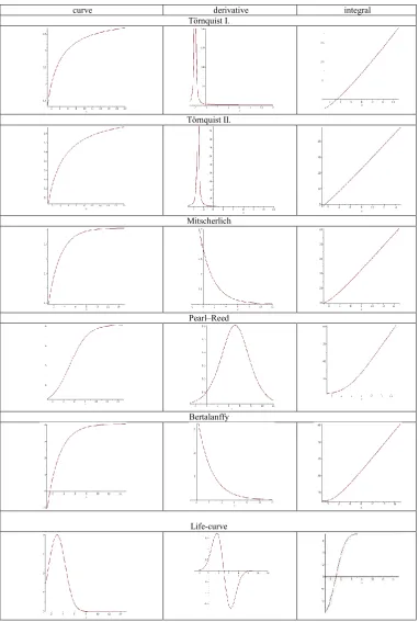
Six different types of sigmoid function are compared: two types of Törnquist- curves, the Pearl–Reed logistic curve, the Mitscherlich-curve, the growth curve of Bertalanffy, and the curve of the life function. After the comparison of the curve

shapes, more conclusions can be derived from the analysis of the derivatives and integrals of the curves. The „sigmoid” name given to these curves refers to the S-like shape of the curves, with a saturation-like behaviour. In infinity these curves approach a constant value, while before that the curves show a relatively quick development or increasing tendency.

The curves are frequently used to describe the development of biological species, social phenomena, market development, or product life. The iteration history of evolutionary type optimisation algorithms has also a sigmoid shape. Sometimes these curves are called „learning functions”, therefore they can be also used for evaluation and comparison of different

Table 1. The shape of the investigated sigmoid curves, their first derivatives and integrals

curve derivative integral

Törnquist I.

Törnquist II.

Mitscherlich

Pearl–Reed

Bertalanffy

Life-curve

student- teams and groups. Regarding these different fields of scientific life, it is possible to assign several meanings to a given characteristic of a curve and this meaning could be re-interpreted in an-other field, giving new meaning to that characteristic. This can give possibilities for finding new features with which to compare, evaluate or rank different achievements of groups or teams,whether it be in engineering education, sport or several competitions. On the basis of these points of view a complete system of evaluation can be elaborated. Using this system any jury can resolve difficult situations or difficult decision-making cases and they can explain their decisions numerically and in more detail. This makes the decision-making process more objective and accurate. In the first step let’s collect the sigmoid curves which can be applied to this process, writing the first derivative and the integral of the curves, as is shown in Table 1.

a.) Törnquist I. curve (Törnquist, 1981):

equation of the curve: ( ) = , first derivative: ( )=

−

( ) , integral: ∫ ( ) = − ( + ) (1)

b.) Törnquist II. curve (Törnquist 1936):

equation of the curve: ( ) = ( ) , first derivative: ( )=

− ( )

( ) , integral: ∫ ( ) = − ( − )ln ( + )

(2)

c.) Mitscherlich-curve (Mitscherlich 1909):

equation of the curve: ( ) = (1 − ),first derivative:

( )

= , integral:∫ ( ) = + (3)

d.) Pearl–Reed (logistic) curve:

equation of the curve: ( ) = , first derivative:

( )

=

( ) , integral: ∫ ( ) = − ln( ) +

ln (1 + ) (4)

e.) Bertalanffy-growth curve:

equation of the curve: ( ) = (1 − ), first

derivative: ( )= , integral:∫ ( ) = +

(5)

f.) Life-curve :

equation of the curve: ( ) = _{( )} , first derivative:

( )

= − ( _{( )} ) , integral: ∫ ( ) = √ ( −

) , erf( ) =

√ ∫ (6)

erf(x)is the Gauss-error function (Andrews 1998).

The six investigated curves can be split into two groups: curves with one point of inflexion (saturation or growth shape curves, such as Törnqist I and II, Mitscherlich, and Bertalanffy) and curves having two points of inflexion (the Pearl–Reed curve and the integral of the life-curve), where the second point of inflexion can describe some real phenomenon, when investigating the development history of the groups. Regarding the curve, its first derivative and its integral, more difference

can be found: in case of the curves having two points of inflexion, one of these three cases gives the „bell”-shaped curve, which provides several opportunities to derive further conclusions and to develop different features for the comparisons. Since the real studied phenomenon can be either a growth-curve type, or a logistic curve, it is enough to select two curves (Bertalanffy and Pearl–Reed) from the six for the further investigations. Analysis of the life- curve can give special results (response spectrum and eigenvalues of the groups, Lorentz-profile, spreading characteristics), so this curve will be studied separately.

Approximation of the curves

During the investigations, the data determining the given phenomenon are available in sets of discrete values. For the study of achievements of student groups the most important data is the number of students with a certain result (number of points, grade, etc.). These data will be approximated by the curves, by using the method of least squares, determining the

parameter values of K, r, c which give the best approximation.

After the approximation process, when we know the effects of these parameters on the shape and behaviour of the curves, it is possible to start the comparison and evaluation process, translating these characteristics to the efficiency, quality and quickness of the groups. This acts as the basis of an objective and detailed evaluation and comparison process. During the method of least squares it is necessary to approach the given

discrete values (xi, yi), i = 1, 2, 3, … , n, by a function y* =

f(x) , while the parameters of the curve should give the minimum possible value of the sum of the squares of the

differences. This means that regarding the function values f(xi)

= y*i , we have to find:

= ∑ ( − ∗) = . (7)

The minimum is possible if the first derivative of the function

H is 0, therefore:

= 0, = 0, = 0, this gives three equations for the

three unknowns K, r and c, so it is possible to find the

parameters for the best approximation. Another possible way to

find the minimum of H as a function of the three parameters, is

to solve the problem as an unconstrained minimisation task of

H using the three parameters as design variables. In this paper

coefficient’s absolute value to 1, the better the correlation between the data and the approximation curve. If the regression coefficient is negative, it shows a decreasing tendency, while positive value shows an increase. This means that the conclusions derived from a curve having „weak” regression coefficient will be not „true”, „strong” or accurate enough, but the conclusions derived on the basis of a curve having good correlation will be true and adequate, or„ strong”. For calculation of the regression coefficient, the curve equations need to be transformed into linear form for both of the selected functions. Linear transformation of the Bertalanffy- function:

( ) = (1 − ), = ( ), + =

( )

, (8)

teherefore the linear function for the Bertalanffy- curve is:

y* = a + bx , where a = ln c , b = -r .

The linear transformation of the Pearl- Reed function can be done in a similar way:

( ) = , ( )

( ) = , + =

( )

( ) ,

y* = a + b x (9)

The regression coefficient can be calculated as:

= (10)

where:

= ∑ , = ∑ ∑ , = ∑ ,

= (∑ )

= ∑ , = (∑ ) .

In equation (10) one can calculate the linear regression coefficient of the y* transformed function determined in equation (8) or (9), but for simplicity we returned to the y notation.

Comparison of two groups of engineering students

For the comparison of the results of two different student groups, a subject was selected which is being taught to several groups, with relatively large class sizes. The reason of that was to provide large amount of data in each group for the curve approximations, and to have at least two groups of the same subject for comparison. During the comparison and evaluation of student results, our objective was not the characterisation and evaluation of the individuals of the groups, but to work out several features for comparisons, with concrete meaning regarding the groups and their achievements, which could be used later – after some „translation” and rethinking – for other fields (sport results or evolutionary optimisation algorithms). The results of the students are analysed without name and without any personal data, only the values and the number of students having the same result will be investigated when deriving the conclusions and during the elaboration of the points of view for comparisons and evaluations. All of the comparisons and the conclusions referred to the groups and to the results of the groups, not to individual group members. This is to respect as much as possible the rules and moral or ethical

prescriptions concerning the individual rights, and personal information of the students. The resulting points of two different groups of 1st year mechanical engineering students taking the same course and writing the same test are as follows (maximum possible points: 50) :

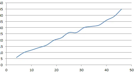
Group I. First it is necessary to write the resulting number of points in an increasing order, taking into account how many students achieved the same resulting points (total number of students in the group: 64, average point obtained: 23.67). The points in increasing order:

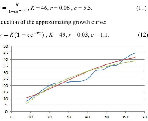
2,4,6,6,6,7,7,8,8,11,11,12,14,14,14,16,18,20,20,20,20,21,21,22, 22,22,22,22,22,23,23,23,23,23,23,23,23,24,24,25,25,26,28,31,3 1,31,32,32,33,34,34,35,36,36,36,36,36,36,39,41,41,42,44,45. The growth (or evolutionary) nature of the curve of the results shows up if it is drawn as a „history” of the best results, as a function of the investigated number of the students, on the basis of the increasing order of point results (Figure 1). Although the curve shows some saturation- behaviour, it does not seem to be a typical growth function or a typical logistic function. This explains why it is necessary to see and compare the regression coefficient for both of these curve types. After the approximation process using the method of least squares, the approximation curves can be seen in Figure 2. In Figures 1 and 2 the horizontal axis of the graph means the cumulative number of students taken into account for the given points, which can be read on vertical axis.

Figure 1. Curve of results of Group I. (points as a function of the number of investigated students)

Equation of the approximating logistic curve:

= , K = 46, r = 0.06 , c = 5.5. (11)

Equation of the approximating growth curve:

= (1 − ) , K = 49, r = 0.03, c = 1.1. (12)

The correlation coefficient for the logistic function is -0.93, for the growth function -0.91. On the basis of the regression coefficient results, the first conclusion is that concerning the resulting curve of Group I shows better correlation with the logistic function, which means that the curve must have two points of inflexion. The conclusions and features for comparison will be „stronger” on the basis of the logistic function than those using the growth function for Group I. and therefore the logistic curve will be used to derive the conclusions and to elaborate the points comparison. Regarding Figures 1 and 2, it is obtrusive that the resulting curve has an almost horizontal section somewhere in the middle and a short but steeply increasing section at the end. The steep increase is caused by a small number of students (one or two) with very good result, which are outstanding comparing to the „normal” behaviour of the curve (of the group). These students are probably talented, diligent students, so it worth giving them more tasks or inviting them to student competitions, other student research works, projects, etc. (talent- treatment, talent nurturing system (Bérczes 2015)).

The horizontal section of the curve is caused by a group of students with average points, they do only „what is enough” and no more. These students could be a good target group for a special „challenging” program or special consultations increasing their interst and results, because this could be one of the most efficient ways to increase the overall result of the group. Around 20 points, there is an increased motivation stage, where the pace of the increase is a little bit higher, than the „normal”. This 20-point limit was the „acceptable” rank or passing mark, which could be behind this increased motivation. This motivation will decrease around 22- 23 points result. The fact that the logistic function has a better regression coefficient than the growth function does indicates that the beginning of the curve (showing the failing marks) has a considerable effect, that is, in the group there are some students with probably insufficient motivation (or interest or knowledge, etc.) and maybe that’s why their result was not enough to pass the exam. The smaller the correlation of the growth function (comparing to the logistic function correlation), the stronger this phenomenon. The proposed comparison process in this paper makes it possible to compare and evaluate numerically the strength of this phenomenon, which will make easier for a teacher to decide if it is necessary to organise a repetition course or more consultations for these students in order to improve their results or help them to reach the passing mark (searching for close-up methods).

Let us see the effects of the curve parameters (K, r, c): The

value of the parameter K is the theoretically best possible result

in the group, this shows the achievement capacity of the group.

Comparing several groups, the team with the highest K value

can achieve the best result, so this group will be the „record

holder”. The value of the parameter r shows how „quick” or

steep is the development or the increase of the results in the group. If this parameter is higher, it means that one can find more students in the group with good results and a smaller

number of students with unsatisfactory results. The parameter c

has a mixed effect on the shape of the curve: it can modify the maximum value and the development speed, too. The numerical value of these parameters can be very important when comparing different groups or teams, because they can show even very small differences between the groups numerically, giving the possibility to a jury to make objective, accurate decisions and comparisons.

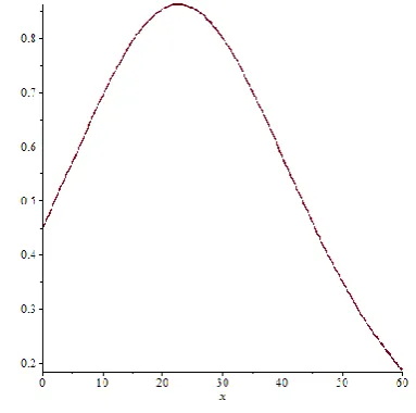
Regarding the first derivative of the approximating curves, for the growth curve the derivative (see Table 1) is monotonically decreasing, showing that the pace of the increase is decreasing, if we see higher point results. The first derivative of the logistic function (Figure 3) is more interesting: it has a bell-shape, with a maximum value, which shows the place of the maximum development pace. The equation of the curve:

,₌ . .

( . . ₎ (13)

The shape of the curve:

Figure 3. First derivative of the logistic curve approximating the results of Group I

It is interesting, that the derivative has its maximum near to the average value of the group results (place of maximum: 26, average: 24). The maximum of the bell-curve shows the highest development pace of the group, this could be also a very good basis of a comparison between groups. The place of the highest speed can be found also in Figure 1 or 2, it can be seen that after that place the development pace is decreasing. The place of the highest development pace can be in connection with the highest motivation part of the curve, too, so the highest development pace can show numerically also the most highly motivated part of the group. For comparison, it is necessary to see the results of the other group, too, in order to develop the criteria for the evaluation and comparison of the group achievements:

Group II. Number of students in the group: 50, average point

result: 23.98. Point results in increasing order: 1,2, 4,6,8,9,10, 11,12,12,13,14,14,15,16,16,17,20,20,20,22,22,22,23,25,26,26,2 6,26,27,29,30,31,31,31,31,32,32,32,35,36,38,38,39,42,45,45,47 ,48,49. On the basis of these data a characteristic curve of the group can be drawn, which can be seen in Figure 4.

Equation of the approximating logistic curve:

= , K = 46 , r = 0.075, c = 5.5 (14)

The equation of the approximating growth function:

= (1 − ) , K = 50 , r = 0.03 , c = 1.02 (15)

By using our approximation algorithm based on the method of least squares, the approximation functions can be found in Figure 5. The regression coefficient for the logistic function is -0.94 and, for the growth function it is -0.92, better than in the case of Group I. On the basis of the results of the approximation, it can be concluded that the logistic function correlates better with the data than the growth function, therefore this function will be used. The result curve of Group II is similar to that of Group I, but it contains smaller waves and fewer horizontal sections. This means that the development history of the results in the group is smoother, than in the other group, the lower motivation part is missing around 22-23 points. At the end of the curve the steep increase caused by excellent students is a little stronger and the theoretically possible highest result of the group is considerably higher (49 in this group, 45 in the other group).

The better correlation given by the logistic function means that here also it is possible to find a sub-group of students with low point results. But the slightly better correlation of the growth function means that in Group II this phenomenon has less importance (-0.92 is better than -0.91), even if the number of the failed students is 17 (34%), which is higher than for Group I (17 failed, 26.5%). This is an other example of how this evaluation system can show very small differences and the numerical representation of the characteristics can be useful to help in the decision making process.

Figure 5. Approximation of the result curve of Group II. (solid line: logistic curve, dashed line: growth curve)

Regarding the parameter K, there is no difference between the

two groups (K = 46 for both), so the „achievement capacity” of

the groups is similar. (It must be noted that for the growth

function, the K = 50 value for Group II is slightly better, than

the K = 49 for Group I, and the correlation of the growth

function is a little better for Group II than for Group I. This means, however, that the logistic function shows a „stronger” basis for the comparison, since it is possible to find a slight

difference using the growth function, too.). The value of r is

higher for the Group II, therefore here we can find the higher pace of development, so specifically this group contains fewer

students with insufficient results. The value of c is the same for

both groups, and cannot give us a means for comparison in this case.

In Group II, the more highly motivated students have results around 25 points, so this is better than for Group I. This increase could be a sign of some „higher quality” of the group (knowing that this could be a function of many parameters, for example in which part of the day is the material taught, when was written the test, effects of many individual differences (Tóth 2014), etc.). The average points are also better for Group II, so these results suggest that Group II could be the winner at the end. But before making the final decision, let’s see the bell-curve of Group II:

The equation of the first derivative of the logistic function (14) is as follows:

,₌ . .

( . . ) (16)

The bell- shaped curve of the Group II can be seen in Figure 6.

Figure 6. First derivative of the logistic curve of Group II

The place of the maximum of the logistic curve is the same for the groups (23 and 24), but the value of the maximum is higher for Group II (0.86 compared to 0.69 for Group I) so Group II can reach a higher pace of growth.

Comparison of the life- curves

Comparing the life curve (or Hubbert-curve) to other sigmoid-like functions in Table 1, it can be seen that the sigmoid shape is occurs for the integral of the function, not for the function itself. Another difference is that for creating the function, instead of results expressed as points, the marks will be used. In Hungary a 5 step ranking system is used. In this system 1 means an insufficient result (fail), 2 means the minimum required result (pass), 3 is a satisfactory mark (average), 4 is above average and 5 is excellent.

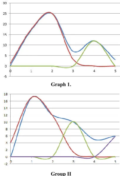
The requirement for the pass mark (2) is around 40% of the maximum points, and normally equidistant intervals will be used for deciding how many points will be necessary for marks of 3 and 4. Using the 5-step ranking system, the points of the groups can be translated into marks. The life curve of a group will show how many students received the given mark. The life curves of the groups are shown in Figure 7 (horizontal axis shows the marks from 1 to 5 and vertical axis shows the number of students).

Graph 1

Graph 2.

Figure 7. Life curves of the two groups

In the life curve, the saturation character of group behaviour will be signalled by the integral of the life curve. This sigmoid curve is different from the sigmoid functions shown in Sections 2- 4, because the coordinate axes are different. This causes the meaning of the parameters to change also. In the integral

function of the life curve, the parameter K means how many

students we have to investgate in order to reach the given

result, therefore the smaller K will be better, because for good

results a smaller number of students is enough. The name of this function is the Gauss- error function, so using this notation

one can say that if K is smaller, the „error liability” of the

group is lower. If the parameter r is higher, the curve is steeper,

meaning that the error-making tendency is smaller in that

group. The parameter c here also has a „mixed” effect, it can

modify the effect of both K and r.

The meaning of the bell- shaped function also change in this case: here the bell- function shows the expectable characteristic value(s) of the group results and it is possible to see the spread of the results, too. In Figure 7, one can find two characteristic values for Group I and three for Group II. Approximating the life curve of the groups, each characteristic value needs its own approximation curve, prompting us to call these values „eigenvalues” of the group, and the approximate eigencurves are similar to and can be called Lorentz- functions of the groups (Figure 8). On the basis of these curves, we can say that the eigencurves and the system of eigenvalues of the groups together can describe the response spectrum of the group (Figure 9). This is an analogy to vibrating systems: the vibrating system is the group and the exam test is the excitation. Around the eigenvalues a kind of „resonance” is present, and the width of the Lorentz- curve is in connection with a kind of „damping”. The eigenvalue is where the life curve has a maximum (several local maxima are possible). For higher eigenvalues, the result which can be attached to this

eigenvalue is better, so in case of higher eigenvalues, the higher „amplitude” value means a better characteristic for the group, however, for smaller eigenvalues the lower amplitude is better, because in this case a smaller number of students can be associated with that weaker result. Regarding Figures 7, 8 and 9, it is possible to measure and compare the width of the eigencurves around a certain eigenvalue. Numerically it is possible to define the „width at half maximum” of the eigenvalue, which is in connection with the spreading or dispersion of the results around that eigenvalue. This will show the significance of that eigenvalue. In the comparison process, the smaller significance of a given eigenvalue is better if the result associated to the eigenvalue is smaller. Larger spreading is better if the associated result is higher. This can give further useful points of view for comparison of the results of several groups. The derivative of the life curve is also connected with the dispersion of the results, so if we use the name Lorentz function for the eigencurves, it is possible to calculate the first derivative of each eigencurves, which will be the dispersion function of that eigenvalue (Figure 9), which can be called the Lorentz- profile.

Graph 1.

Group II

Figure 8. Lorentz- functions and spectrum of the groups

Equations of the eigenfunctions: ( ) = _{( )} (17)

Group I

Eigenvalue 1: K = 29.0r = 1.65 c = 1.1 Eigenvalue 2: K = 12.0 r = 4.0c = 4.0

Group II

Eigenvalue 1: K = 18.5 r = 1.3c = 0.95 Eigenvalue 2: K = 10.1 r = 3.0c = 2.2 Eigenvalue 3: K = 6.0r = 4.97 c = 0.95

Equations of the derivatives and integrals of the curves can be created by using equation (6). The integral of the Lorentz

function in Table 3 is supposed in the following form: y = K1

Figure 9. The spectrum, eigenvalues, Lorentz- functions and Lorentz- profiles of the groups

Table 2. The significance factors calculated for the eigenvalues of the groups

Eigenvalue Group I Group II

E1 71.4 42.1

E2 28.8 27.0

E3 ---- 52.5

Table 3. Comparison aspects of the evaluation system

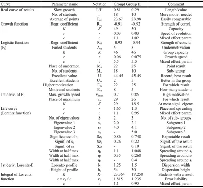
Curve Parameter name Notation GroupI Group II Comment

Real curve of results Slow growth L/H 0.81 0.29 Length/value

No. of students n 18 10 More motiv. needed

Average of points Pav 23.67 23.98 Easily comparable

Growth function Regr. coefficient Rkg -0.91 -0.92 Strength of correl.

K K 49 50 Capacity

r r 0.03 0.03 Speed of evolution

c c 1.1 1.02 Mixed effect param.

Logistic function (Fl)

Regr. coefficient Rkl -0.93 -0.94 Strength of conclu.

Failed students Am 5 3 Undermotivation

K K 46 46 Group capacity

r r 0.06 0.075 Growth speed

c c 5.5 5.5 Mixed effect param.

Place of undermot. Mh 22 25 Point result

No. of students Msz 18 10 Sub- group

Excellent value U 44-45 45-49 Record, best result

Excellent students Usz 2 5 Better in the group

Higher motivation Em 22 25 For which result

Motivated students Esz 8 5 How many students

1st deriv. of Fl Max. growth speed vfmax 0.7 0.85 High motivation

Place of maximum vm 29 26 For which result

Life curve (Lorentz function)

K K 29 18.5 At most signi. eigenv.

r r 1.65 1.3 Place and spreading

c c 1.1 0.95 Mixed effect param.

No. of eigenvalues S 2 3 No. of sub- groups

Eigenvalue 1 s1 2.0 2.1 Subgroup 1

Eigenvalue 2 s2 4.0 4.1 Subgroup 2

Eigenvalue 3 s3 - 5.0 Subgroup 3

Significance of s1 Sz1 0.86 0.748 Expectable result

Signif. of s2 Sz2 0.26 0.22 Signif. of the result

Signif. of s3 Sz3 - 0.19 Signif. of the result

Width at half max. η1 1.1 1.048 Spreading around s1

Width at half max. η2 0.35 0.268 Spreading around s2

Width at half max. η3 - 0.4 Spreading around s3

1st deriv. Lorentz-f. Lorentz- profile bd 1.25 1.5 Dispersion width

Height of profile hd 54 30 Dispersion height

Integral of Lorentz function

K K1 23.364 17.258 Students with a result

r = r1 / c r1 1.815 1.235 Error liability

c c 1.1 0.95 Mixed effect param.

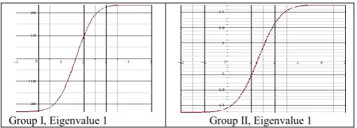
It is interesting to see that the dispersion curve has zero value where the Lorentz- curve has its maximum, in case of each eigenvalue. Multiplying the eigenvalue by the „amplitude” and by the width at half maximum, the resulting number can be called the significance factor.

Group I, Eigenvalue 1 Group II, Eigenvalue 1

Figure 10. Error functions of the groups (integral of the Lorentz function)

This factor can be relatively high, if the eigenvalue is a good result, many students achieved that good score and the spreading is high around this eigenvalue. Since a relatively smaller result reached by many students and having high spreading around it can also give a high significance factor, the teacher or the jury has to select between the eigenvalues to determine, which they will treat as more significant. Ranking and comparing the eigenvalues one by one for the groups, as well as reading and explain the numerical values of the significance factors of each eigenvalue, can help also in forming the final decision and can help to discover sub-groups in the group which should be treated or helped by special methods and consultations (talented students, failed students, low motivated average, etc.). Table 2 shows the significance factors of the eigenvalues of the groups, while Figure 10 shows the sigmoid functions (the integral of the Lorentz-function, also called error function), calculated for the first eigenvalue of the groups. The highest significance factor resulting for Group I is 71.4 at 1.75 eigenvalue, while for Group II this is 52.5 for the eigenvalue of 5. On the basis of the curves and characteristics shown in previous Sections, it is possible to collect all the possible viewpoints of the proposed evolutionary system for the comparison and evaluation of the results and achievements of groups (Table 3). All in all 38 points can be collected and elaborated on the basis of the curves and characteristics of the groups, and of these 32 are „decision- friendly”, which means hat it can be given to one of the groups because it is better from that point of view. From the 32 points of view, Group I performed better in 8 and Group II in 24. Therefore it can be concluded that the winner of this comparison and evaluation process is Group II. We could say, based on the aspects, 25% Group I and 75% Group II, so the Group II wins 3 to 1 , if we want to give soccer-like results.The comparison process of Group I and Group II shows the efficiency of the proposed system to display and evaluate numerically even very small differences between the groups or between the results or achievements of the groups. This could be a significant help to a jury in deciding the winning group, but also for teachers of the groups to find the sub-groups possibly needing some special treatments or consultations (for talented students, failed students, etc.). Comparison of several groups also helps to evaluate or to find the real weight of the necessity of this kind of special attention.

DISCUSSION

In this paper an evolutionary based evaluation and qualification system (EBSYQ) is proposed for the comparison of group or

team results or achievements. The evolutionary basis of the system comes from the application of sigmoid curves (growth curve, logistic curve), since these curves can be used also for the description of the iteration history of evolutionary type optimisation algorithms. Thirty-eight different points of view are collected for the comparison of the group results. On the basis of these comparison criteria it will be very easy for a teacher to find the appropriate target–sub-group for a given type of special work or consultation activity (for talented students, competitions for outstanding students, increasing the interest and attendance of average students, or special consultations or remedial work for undermotivated or failed students). The application of this system during a competition among groups (or selection of possible applicants for a job, etc.) makes possible to the decision makers to see the existing differences more clearly, even if they small, and hard to detect or notice in other ways. This could help a jury or decision makers to make decisions in more objective and accurate manner, numerically evaluating and comparing each point of view during the comparison process. The efficiency and usage of the system is demonstrated through a real-life example: two student groups writing the same test were compared. Analysis of the example by the EBSYQ system proves that the system can show even very small differences clearly and numerically, which can be useful help even in case of close competitions. The first step of the usage of the proposed system is to obtain the data as points. This can be the test results of the group members but if it is a special competition and there is no written test it is necessary to build the series of most important requirements or objectives and the points can be given to the group members. This will be the only one subjectivity in the system.

also very useful aspects and viewpoints to the final decision to a jury or to design special consultation to be given by a teacher. The first derivative of a Lorentz-function gives the dispersion function, the Lorentz-profile. The shape, the height and width of the Lorentz profile can give useful information about the distribution of the results which can be in connection with the strength of the cohesion or cooperation of the group members. The integral of the Lorentz- function gives the error- function of the group, which is better if it is steeper, because in this case the maximum result of the group is achieved quicker. The numerical evaluation of each decision criteria makes also possible to assign a weighting to the viewpoints, in this way some skills or knowledge or type of results can be more emphasised to fit the goals or objectives of the given competition or selection procedure (selection for jobs, finding a target group for further educations, fulfilling special requirements of competitions, design of special consultations, etc).

Application of the EBSYQ evaluation system of group achievements can be useful in several decision-making situations in scientific and education fields, resulting more accurate and more objective decisions, which can give advantages to teachers in finding more precisely the target groups for special treatments and consultations, or to decision makers in making better decisions more easily and quickly, to the students or to the members of evaluated groups to win and obtain with higher probability and on more objective basis the prize they are compete for and to arrive more surely in a position where they can enjoy the results of their long, hard and diligent work. Further research in this theme could be to extend this system to international student group competitions or other fields of life: analysis and comparison of sports results (groups, individuals) and analysis of evolutionary type optimisation algorithms.

Acknowledgements

The author of this paper would like to thank Dr. Gabriella Bognár Vadászné, professor, director of the Institute of Machine and Product Design at the University of Miskolc for her useful suggestions and helps, to Ms. Klára Benyó, university tutor of engineering in the Institute of Machine and Product Design at the University of Miskolc, for making available the necessary data of student groups for this research and for her useful suggestions and helps. The described study was carried out as part of the EFOP-3.6.1-16-00011 “Younger and Renewing University – Innovative Knowledge City – institution development of the University of Miskolc aiming at intelligent specialisation” project implemented in the framework of the Szechenyi 2020 program. The realisation of this project is supported by the European Union, co- financed by the European Social Fund. The research work presented in this paper is partly based on the results achieved within the following projects:

 HEIBus 575660-EPP-1-2016-1-FI-EPPKA2-KA (Smart

HEI- Business Collaboration for Skills and

Competitiveness) ERASMUS+ International Project (HEI = Higher Education Institutes).

 TÁMOP 4.2.1.B-10/2/KONV-2010-0001 in the framework

of the New Hungarian Széchenyi Plan.

 The realisation of this project is co-supported by the

European Union and co-financed by the European Social Fund. The author would like to thank to all these programs and persons for helping to finance and to realise this research work.

REFERENCES

Andrews, L. C. 1998. Special Functions of Mathematics for

Engineers: SPIE Optical Engineering Press: Bellingham, USA.

Bérczes, R. 2015. “The Improvement of Higher Education Quality and Talent-nurturing with Scientific Students’

Association (SSA) Commitment” Acta Polytechnica

Hungarica, Vol. 12. No. 5: 101-120.

Bertalanffy, L. 1960. Principles of Theory of Growth. In:

Fundamental Aspects of Normal and Malignaent Growth. Amsterdam. pp. 137-259.

Hubbert, M. K. 1956. “Nuclear Energy and Fossil Fuels.”

Drilling and Production Practice, American Petoleum

Institute & Shell Development Co. Publication, No. 95: 9-11.

Kehl, D.; Sipos, B. 2009. Approximation of logistic function, growth function and life function by Excel command

language. Statisztikai Szemle [Statistics Survey], Vol. 87.

No 4. (In Hungarian).

Lorentz, M. O. 1905. Methods of Measuring the Concentration

of Wealth.Publications of the American Statistical

Association. Vol. 9 No. 70: 209- 219.

Mitscherlich, E. A. 1909.: The law of minimum and the law of

diminishing soil productivity. (In german).

Landwirtshaftliche Jahrsbücher, 38., pp. 537-552.

Nelder, J. A., Mead, R. 1965. A simple method for function

minimisation. Computer Journal 7. : pp 308- 313. doi:

10.1093/comjnl/7.4.308

Pearl, R.; Reed, L. J. 1920. On the Rate of Growth of the Population of the United States since 1790 and its

Mathematical Representation. Proc. of the National

Academy of Sciences. Vol. 6. No 6. pp. 275-288.

Törnquist, L. 1936. The Bank of Finland’s Consumption Price

Index. Bank of Finland Monthly Bullettin,10, 1-8.

Törnquist, L. 1981. Collected scientificpapers of Leo Törnquist. Research Institute of the Finnish Economy. Series A. ISBN 978-951-9205-74-8, 1981.

Tóth, P. 2014. “The Role of Individual Differences in

Learning”. Acta Polytechnica Hungarica, Vol.11, No. 4:

183-197.

*******