Fish fast-starts are sudden accelerations from rest associated with prey capture and escaping from predators. Weihs (1973) defined three kinematic stages for fast starts: a preparatory stage in which the straight-stretched fish bends into a Cor S shape, a propulsive stage in which the fish executes a reverse bend, and a variable stage, which may be a subsequent power stroke, steady swimming or unpowered coasting. Large forces must be generated when a fish with a straight body suddenly whips its tail to the side and straightens out again (i.e. fish must generate a forward thrust from an essentially sideways tail motion). Harper and Blake (1990) studied the kinematics of fast-starts using ciné film and accelerometry. They found maximal accelerations of 25 g, where g is the acceleration due to gravity, for northern pike Esox lucius. Later, Frith and Blake (1991, 1995) applied Weihs’ (1973) hydromechanical model to kinematic data to determine the energetic cost and efficiency of pike fast-starts. Unfortunately, these studies did not measure the actual forces directly, so conclusions regarding muscle power and efficiency can only be inferred.
Ahlborn et al. (1991) employed a simulated fish-tail apparatus to visualize the flow during fast-starts and proposed a vortex production–destruction model to determine the thrust forces. They concluded that the propulsive forces are associated with a change of rotational momentum of vortex structures at the tail fin, rather than with linear displacement and acceleration of the fluid as modeled by Lighthill (1971) and Yates (1983).
The model of Ahlborn et al. (1991) suggested a quantitative difference in thrust production of the initial sideways flip and the return stroke of the tail. Although
kinematically identical, the sideways flip would essentially set up a vortex and thereby exert a sideways reaction force onto the fish, and the return stroke would essentially stop the rotational motion of the vortex and produce forward thrust. It was noted that the thrust would be even greater if the return stroke inverted the direction of the initial vortex rather than only stopping it. For this reason, we refer to the model as the ‘momentum-reversal model’.
The flow-visualization experiments of Ahlborn et al. (1991) did show the production and subsequent destruction of the initial tail tip vortex. However, the gravity-driven mechanism of the apparatus did not allow the motion parameters to vary, and no force measurements were made. The model failed to recognize that energy expenditure would be minimized if the primary vortex was exactly inverted, and it did not account for how the vorticity induced by the forebody would interact with the propulsive mechanisms described.
Here, we report new measurements of the thrust force, Fx, and the accumulated impulse, J(t), generated by fish tail motions during the start-up phase in the intended forward ‘swimming’ direction. J(t) is defined as:
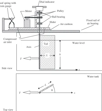
where t is time. The experiments were conducted using a completely redesigned tail simulation apparatus (Fig. 1). The tail-fin motion is now controlled by a computer and the tail angle, φ, is measured as a function of time. Furthermore, we extended the momentum-reversal model by showing how (1) J(t) = ⌠
⌡
t
0
Fxdt ,
Printed in Great Britain © The Company of Biologists Limited 1997 JEB1136
Measurements of the thrust and forward impulse of a simulated fish tail and mathematical modeling indicate that the propulsive forces of fast-start swimming can be optimized by three different effects: (i) exactly inverting the tail tip vortex that is generated with the initial stroke, (ii) using a moderately flexible tail, and (iii) introducing a
specific delay between the initial stroke and the return stroke. Experiments were performed with a new computer-controlled fish-tail simulation apparatus, and the results confirm the theoretical predictions of a previous study.
Key words: fish, swimming, fast-start, thrust, vortex, momentum.
Summary
Introduction
EXPERIMENTAL SIMULATION OF THE THRUST PHASES OF FAST-START
SWIMMING OF FISH
B. AHLBORN1, S. CHAPMAN1, R. STAFFORD1, R. W. BLAKE2 ANDD. G. HARPER2,*
1Department of Physics, University of British Columbia, Vancouver, British Columbia, Canada V6T 1Z1 and 2Department of Zoology, University of British Columbia, Vancouver, British Columbia, Canada V6T 1Z4
Accepted 13 June 1997
energy expenditure can be minimized and how vorticity induced in the flow by the forebody actually helps propulsion.
Propulsion by reversal of momentum
To appreciate our extension of the momentum-reversal model, its principal features are first reviewed. The model predicts the thrust and power production of fish with rather stiff bodies, to which Lighthill’s (1971) slender-body model cannot be readily applied. The model starts from first principles by describing the angular motion of the fluid elements near the tail tip. We assumed that the tail moves sideways in the initial stroke and immediately thereafter returns to the straight position in the return stroke. The first sideways flip of the tail presumably generates a vortex with some velocity distribution u(x,y,z)=rω(x,y,z), where r is the distance from the centre of rotation of the vortex and ω is the angular velocity of the vortex, resulting in the angular momentum Gi:
where dm is the mass element in the fluid and ωiis the angular velocity at which a solid body with the same mass moment of inertia, Ii=∫r2dm, would rotate in order to have the same angular momentum. Giis produced by applying a torque, Γ=Fyx1, with an essentially sideways force, Fy (Fig. 2A). This vortex is subsequently stopped or even inverted by the application of Γ with an essentially longitudinal force, Fx, exerted during the next phase of the tail motion (Fig. 2B). The fish makes use of the inertia initially imparted to the water. In this way, the induced vortex acts like a ‘stepping stone’ against which the fish can push to gain forward momentum. The torque, Γ, which changes the angular momentum of the vortex from the initial value, Gi, to some final value, Gf, is modeled as force, Fx, applied at distance y2 from the center of rotation. Fish may swim in a stealthy manner that minimizes the vorticity left in the wake (Ahlborn et al. 1991), a special case where Gf=0. The propulsion force then becomes:
where ∆t is the time during which the torque Γis applied. With (3) Fx=
1 y2
1 y2
1 y2
Gf−Gi
∆t
0 −Gi
∆t
Gi
∆t
= = − ,
(2) Gi=
⌠ ⌡vortex
ωr2dm = I iωi,
AA
A
A
A
A
AAAA
AAAA
AAAAAAAAA
AAAAAAAAA
AA
AA
AAAAAAAAAAAAAAA
A
A
AAA
Dial indicator
Air cushion
AAAA
AAAA
AAAA
AAAA
AAAA
AAAA
AAAA
x T
Ball bearing
Water level Tail
Axis
A
A
A
A
A
A
A
A
A
A
A
A
Leaf spring with strain gauge
Motor Pulley
Slider
Compressed air inlet
L
Fixed rail of air bearing
A
AAA
AAA
AAA
x
φ
T
Water tank Side view
Top view
h
[image:2.609.209.557.73.452.2]L
some simplifying assumptions about the geometry of the induced vortex, the thrust force, Fx, was derived as a function of the tail frequency, f, the deflection amplitude of the tail tip, A, the submerged height of the tail, h, water density, ρ, and an entrainment constant, K:
Fx= (2/π)KρhA3f2. (4) The gravity-driven tail-flip apparatus of Ahlborn et al. (1991), where the return stroke immediately followed the initial sideways flip, showed the destruction of the first vortex. Here, we add three simple considerations to the model.
(i) The increase of force by reversal of the angular momentum
It is easy to see that the force becomes larger if the rotational flow is not only stopped, but is inverted in its direction, so that the final angular momentum, Gf, has the opposite sign to Gi. This gives:
The principle of propulsion by reversal of momentum is expressed in this equation: the inertia induced by the initial stroke is utilized to increase the thrust force, Fx. The model has two extreme cases: either Gi or Gf may be zero. In stealthy motion, Gf=0 and no vortex is left behind. A propulsive force can also be generated if no initial vortex existed, i.e. Gi=0, and only a final vortex with angular momentum Gfis generated. This condition may be present in swimming modes where the fin acts like an airfoil that encounters undisturbed laminar flow. However, it is clear from equation 5 that the thrust force Fx will then be smaller than when some angular momentum existed before the return stroke was applied. It is of interest
that momentum inversion carries no energetic penalty. In fact, the energy expended is minimized if a specific value is chosen for the final angular momentum Gf.
(ii) The energy minimum
The total energy investment, ΣE, for a given impulse, J(∆t)=Fx∆t, is minimized in this model if the angular momentum is reversed in a specific manner. This comes about since the force Fx grows in proportion to the difference between the angular velocities ωi and ωf, while the kinetic energy grows as the sum of the squares of the angular velocities. The proof of this is to express the total kinetic energy of the system as a function of the final angular velocity and calculate the minimum. The total angular kinetic energy, Ei, of the first vortex may be written as a function of the average angular velocity, ωi, of an equivalent solid body and an appropriately scaled mass moment of inertia, Ii′:
In general, this scaled mass moment, Ii′, need not be equal to the quantity, Ii, that defines the average angular velocity. The kinetic energy, Ef, of the vortex left in the fluid after the tail has applied the torque, Γ, can be similarly expressed. The total energy, ΣE, invested in the flip and return motion is the sum of the vortex energy, Ei, initially imparted to the water and the vortex energy, Ef, left behind. The energy minimum Eminis found in the approximation Ii′=Ii, and If′=If, where If is the moment of inertia of the final vortex. The total invested energy is:
ΣE = Ei+ Ef= (1/2)(Iiωi2+ Ifωf2) . (7) The initial angular velocity, ωi=Gi/Ii, is expressed as function of the impulse, J(t)≈Fx∆t, using equation 5:
ωi = [Ifωf−J(t)y2]/Ii. (8) If ωiis substituted into equation 7, the net energy, ΣE, becomes a function of ωf only. By taking the partial differential,
∂ΣE/∂ωf, and setting it equal to zero, the extremum of ΣE is found at the angular velocities ωi,minand ωf,min.
and
It can be shown that the extremum is a minimum with the energy:
From equations 5 and 11, it is evident that tail flips of short duration, ∆t, where the resultant longitudinal force, Fx, is (11) Emin=
Fx∆t ·y2 (Ii+ If)
.
^
(10)
ωi,min= = − ωf,min.
− J(t)y2 (Ii+ If)
(9)
ωf,min=
J(t)y2 (Ii+ If)
,
(6)
Ei= ωi2Ii′.
⌠ ⌡vortex
ωr2dm = 1 2 1
2
(5) Fx=−
1 y2
Gf−Gi ∆t .
− V
-V0
rs
ls U
+
Fy
Fx y2 x1
B A
φ
1
V1
Fig. 2. Flow field around a streamlined aquatic animal with boundary layer velocity profiles on the left side (ls) and right side (rs); V0is the
vorticity generated in the boundary layer and U is the local flow velocity. (A) V1is the vortex resulting from tail motion through angle
φ. Fyis the lateral force exerted by the tail onto the water. x1is the
moment arm of force Fy. (B) The vortex to be inverted by the return
applied with a small moment arm, y2, are physiologically advantageous: they generate large thrust forces and require relatively little energy. For a specified impulse, J(∆t)=Fx∆t, the total energy, ΣE, becomes a minimum when the applied torque exactly inverts the angular velocity (equation 10). Within the scope of the assumptions discussed by Ahlborn et al. (1991), the thrust force at this energy minimum would be twice that of equation 4, namely:
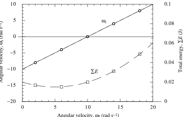
Fx,ΣEmin= (4/π)KρhA3f2. (12) Fig. 3 illustrates how the total energy ΣE (equation 7) and initial angular velocity ωi(equation 8) will vary with the final angular velocity, ωf, if the same impulse, J, is delivered. Values typical of our experiment, J=0.1 N s, y2=0.02 m and
Ii=If=2×10⁻⁴kg m2, are assumed in this example. Note that
ΣEminoccurs when − ωi=ωf≈5 rad s−1.
(iii) The effects of the forebody
The forebody of the animal generates its own flow field. The velocity boundary layer on the left side (ls) and the right side (rs) of a bluff body have strain fields which facilitate the production of vortices with a rotational sense as indicated on Fig. 2A. Such vortices are clearly seen on Freimuth’s (1989) elegant flow-visualization photographs of flapping foils in a background flow. The boundary layer strain fields cause part of the drag acting on the bluff body. In Fig. 2A, the upper space is shown with a negative circulation and the lower half-space with a positive circulation. The sense of rotation is maintained when vortices are shed in the von Kármán vortex street (for a description, see Prandtl and Tietjens, 1934). The meandering wake in the von Kármán vortex street may be considered as an ‘extension’ of the bluff body that separates the rows of opposing vortices.
Vortices produced by the sideways motion of the tail (Fig. 2A) have the same sense of rotation as the flow surrounding the forebody. As the tail flips into the upper half-space, it generates vortex V1containing angular momentum Gi
with a negative circulation. Therefore, it will reinforce any negative circulation that may have come from the forebody. Similarly, if the tail swings into the lower half-space, it will produce a vortex that reinforces the positive circulation arriving from the left side of the forebody. The total angular momentum, Gi, of vortex V1 may, therefore, be attributed partly to the shear forces in the forebody boundary layer (rs) and partly to the lateral force, Fy, exerted as the tail was moved to angular position φm, the maximum deflection of the tail. Since any increase of Gi enhances the propulsive force, the additional vorticity produced by drag on the forebody actually increases this force. In the context of the momentum-reversal model, the strain fields in the boundary layer of the forebody (although contributing to the energetic costs of the motion) become an asset. It appears that nature has managed to extract an advantage out of an apparently adverse situation.
Materials and methods
The experiments were performed in a 100 l aquarium onto which the tail flip apparatus was mounted (Fig. 1). The apparatus was purpose-built as an undergraduate research project. Detailed specifics of the design are available from the authors. A rectangular foil of submerged height, h=15.0 cm, and width, L=5.0 cm, simulates a fish tail. The foil was slid into a metal sleeve acting like a spine which was attached to a round shaft above the water surface. It extended to within 1 mm of the tank floor, so that the water motion could be approximated as a two-dimensional flow. The shaft was driven by a stepping motor, controlled by a personal computer. This allowed the fin to rotate on predetermined paths to create motions resembling those of fish tails, from half-cycles to several full cycles of frequencies selected so that the tail would follow the imposed current waveforms. This accounts for any slack in the motor–pulley system. We concentrate on half-flips, with tail deflection traces as shown in Fig. 4. However, we also recorded some measurements for full cycles in which the tail −20
−15 −10 −5 0 5 10
0 0.02 0.04 0.06 0.08 0.1
0 5 10 15 20
∑E
ωi
Angular velocity, ωf (rad s−1)
∑
Total energy,
E
(J)
Angular velocity,
ωi
(rad s
[image:4.609.245.563.71.272.2]−1)
Fig. 3. Total energy ΣE produced by the tail motion and initial angular velocity ωias a function of final
made one excursion of amplitude φmto the left and to the right of the center line.
In order to measure the thrust force component, Fx, in the negative x-direction as a function of time, the tail rotor was mounted on a platform that rested on air bearings and was restrained to movement in the x-direction. While moving without friction, the platform was held in position by a leaf spring which carried two strain gauges mounted in a Wheatstone bridge. The strain gauges were calibrated to measure the x-component of the force exerted on the tail. When an object of mass m moves at a radial distance, ro, around an axis with velocity v, a centrifugal force, Fr=mv2/ro, is generated where v is directed away from the axis. This effect decreases the measured thrust and increases the drag slightly when the tail is moving. When the tail foil is suddenly stopped at the angle φm, it will produce a force component in the x-direction. For the largest accelerations measured in our experiments, this force was calculated to be 0.01 N and would increase thrust. Since these dynamic effects are in opposition to each other and within the noise level of our measurements (0.01 N), we neglected both.
The computer controlled the lateral deflections of the tail, measured the tail angle as a function of time, recorded the thrust force as a function of time, integrated the thrust force to yield the accumulated impulse, and evaluated the electrical power delivered to the tail fin. The flow field was recorded from below by a 35 mm camera with a motor drive set at 3 frames s−1. The opening time of the camera was recorded simultaneously with the measurement of force and tail position. Typically, we used an exposure time of 0.25 s (see Fig. 4).
A small siphon was mounted at the level of the water surface so that a layer of water could be removed before each run. If this precaution was not taken, the water surface quickly accumulated contaminants that greatly changed its viscosity, thereby affecting the flow pattern. For flow visualization, aluminum particles were filed from a block directly onto the water surface to serve as tracer particles. We found that aluminum particles readily clumped together if they had been prepared long beforehand. Before beginning an experiment,
the tail section of length L=5.0 cm and submerged height h=15.0 cm was oriented in the x-direction, so that the tail angle, φ, was zero.
Aquatic animals are known to use elastic-energy storage mechanisms (Alexander, 1987; Cheng and Blickhan, 1994), and fish tails are highly elastic. Elastic materials obey Hooke’s law where the extension grows linearly with the applied force. Therefore, energy storage is greater in flexible materials than in stiff materials. Consider a force, F, acting on an elastic object with a spring constant, k, deflected to an amplitude, As, so that
F=kAs. The accumulated potential energy, Ep=(1/2)kAs2= (1/2)k(F/k)2=(1/2)F2/k. Flexible materials have a small spring constant and stiff materials have a large spring constant. Therefore, soft materials can store more energy in Hooke’s range of elasticity. In our propulsion model, the energy is imparted to the water and a stiffer tail will transfer energy more efficiently. To investigate the effect of stiffness of fish tails, three tails of different stiffness were used. The tail models all had the same height, h, and length, L, but different stiffness: (i) a stiff tail was made from 0.89 mm thick aluminum, (ii) a flexible tail was fabricated from 0.38 mm bronze, and (iii) a soft tail was made from 0.076 mm brass foil. The flexibilities of the tail models were measured in static experiments. The deflection of the trailing edge of the tail was quantified by horizontally clamping the spine of the tail and pulling the trailing edge of the tail down using weights attached to a thin thread that ran from the spine over the tail. A force of 0.3 N deflected the trailing edge of the soft brass tail by 2.2 cm, and the flexible bronze tail by only 1 mm. Over a range up to 2 N, the aluminum tail would not bend appreciably.
The apparatus was designed to investigate the start-up forces associated with fish fast-starts. Therefore, the platform was only designed to move forward enough to bend the restraining springs and generate a sufficiently strong signal in the strain gauges. In its present configuration, this apparatus is not suited to investigate the steady swimming of fish. We believe that the results obtained for half-flips give a reasonable approximation of the propulsive forces generated during the start-up phase of fish fast-starts. However, the full-flip experiments must be interpreted with caution. Therefore, we refer to them only for 0.2
0.15
0.1
0.05
0
−0.05
−0.1
−0.15
−0.2
Thrust (N)
Drag (N)
Tail angle,
φ
(degrees)
60
40
20
0
−20
−40
−60
φm
0
Spike
1
2
3
4 Thrust Plateau
Tail position
τc
τr
τ0
φf
b c d e
0.2 0.4 0.6 0.8 1 1.2 1.4 1.6 1.8 2
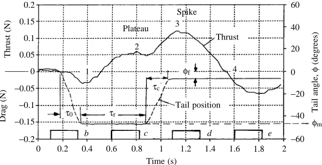
[image:5.609.235.565.72.241.2]Time (s) Fig. 4. Thrust/drag forces and tail angle, φ,
during an excursion of the tail and return to final orientation, φf. Numbers on the thrust
trace indicate the phases described in the text. Tail motion is characterized by excursion (opening) time, τo, resting
interval, τr, and return (closing) time, τc.
interpretation of the last phase of the half-flip experiments. To simulate steadily swimming fish, we would have to use the apparatus in a flow channel or mount it on a cart in a drag tank, so that relative motion between the tail simulator and fluid could be set at appropriate values to mimic steady swimming. Parameters that could be varied in these experiments are the tail deflection wave form, namely the tail angle, φ, as a function of time, and the stiffness of the tail fin. While a real fish moves its tail in a flowing, steadily changing motion (approximating a sine wave), phases of motion resembling the trapezoidal deflection function, φ(t), as depicted on Fig. 4, can be identified from still frames (Bainbridge, 1960; McCutcheon, 1977) and from high-speed films of swimming fish (Harper and Blake, 1990).
Results Force measurements
Experiments with trapezoidal deflection wave forms revealed four very distinct thrust phases both for half-flips (1–4, Fig. 4) and also for full-flips: (1) a negative precursor as the tail moves out; (2) a gradually increasing thrust ending in a plateau as the tail momentarily holds its maximum deflection; (3) a spike as the tail returns towards its rest position; and (4) a gradual decay of the thrust to zero after the motion has stopped. Full-flips have an additional interval of small negative thrust and a large positive thrust spike when the tail returns to its rest position. The model tail did not return exactly to its original position, but came to rest at an angle |φf|>0, so that momentum fluxes in the x-direction exerted a residual drag force. We varied the resting interval, τr, to study the period over which the thrust plateau could be extended. Fig. 5 shows thrust force traces for τr=0.5, 0.7, 0.9 and 1.1 s.
We found statistically significant variations in the drag precursor, probably due to the fact that we did not wait long enough between experiments to let the water settle. Since these variations were random, we concluded that they did not affect
the results. However, it is clear from Fig. 5 that during the rest period the thrust reaches a maximum and then gradually decays, dropping to approximately zero for a resting period
[image:6.609.320.555.157.672.2]τr=0.9 s. It is also evident that, for all delay intervals, the maximum thrust occurs during the return stroke when momentum would be inverted in accordance with our model.
Fig. 5. Thrust forces and deflections for different rest periods, τr,
between the initial excursion of the simulated tail and its return stroke. Rest periods correspond to the curves as follows: (A) τr=0.5 s, (B)
τr=0.7 s, (C) τr=0.9 s and (D) τr=1.1 s.
0.3
0
−0.3
Thrust (N)
0 0.5 1.0 1.5
Time (s)
A B C D
A B C
D Force Deflection
[image:6.609.45.290.530.691.2]τr
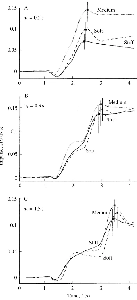
Fig. 6. Calculated impulses, J(t) for different rest periods, τr: (A)
τr=0.5 s, (B) τr=0.9 s and (C) τr=1.5 s. Each consists of three curves
showing mean values for five runs each for stiff, medium and soft simulated fins. The vertical lines intersecting square points indicate the times of peak impulse for each of the fins. See text for further explanation.
A 0.15
0.1
0.05
0
τr= 0.5 s
Medium
Soft
Stiff
0 1 2 3 4
B
0.15
0.1
0.05
0
τr= 0.9 s Medium
Soft
Stiff
0 1 2 3 4
C 0.15
0.1
0.05
0
τr= 1.5 s
Medium
Soft Stiff
0 1 2 3 4
Impulse,
J(
t) (N
s)
The computer recorded the propulsion force, Fx(t), and calculated the total impulse J(t)=∫Fx(t)dt. Fig. 6 shows the mean results from five runs each for each tail-type at the delay intervals τr=0.5, 0.9 and 1.5 s. The effect of increasing τrwas unexpected. The impulse first increases as τris extended and then declines. The maximum impulse is produced with a delay interval of 0.9 s (Fig. 6B), and a large thrust spike is generated when the tail is returned to the starting position, φ=0 ° (see Fig. 4). The thrust is considerably larger than the drag generated in the kinematically similar initial flip. The impulse peaks and then drops (Fig. 6) owing to the decline of the thrust seen in phase 4 (Fig. 4), which we attribute to a misalignment of the tail.
Since fish tails are flexible, we investigated how this property affects thrust. The results show that the impulse is affected by varying both delay time and flexibility (Fig. 6). The impulse, J(t), is a convenient yardstick for comparing the tail types. Two qualitative observations of the effect of tail flexibility can be made. (i) The stiff aluminum tail reaches its maximum impulse first. If the speed of the response is important, a stiff tail has the advantage. (ii) The slightly flexible bronze tail (medium type) generates the highest impulse regardless of the delay time.
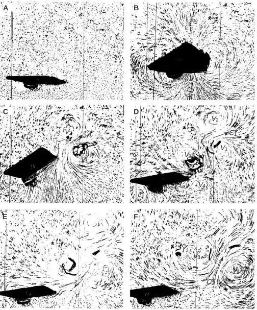
Interpretation of flow-visualization photographs The motion of the fish-tail simulator has two phases which are kinematically identical: the initial stroke and the return stroke. This motion might be expected to generate equal but opposite forces. However, in the Introduction we have shown that this need not be the case. Indeed, the experiments show asymmetric force production. The drag produced by the initial stroke is much smaller than the thrust produced during the return stroke, and there is thrust production during the resting interval τr, when the tail does not move at all (Fig. 4). Furthermore, the impulse can be maximized by selecting a particular delay time τr and a tail of intermediate flexibility (Fig. 6). To investigate these results further, we obtained flow-visualization photographic sequences of the different phases of thrust production. A typical sequence is given in Fig. 7.
The fluid is at rest in Fig. 7A. The tail flips towards the top of the photograph and returns to its rest position. The camera is below the tail so that its base appears to the left of the axis, and the camera views from below when the tail is deflected (Fig. 7B). The intended swimming direction is to the left (negative x-direction).
These flow-visualization pictures show the growth and decay of several vortices. Fig. 8 represents the vortices and induced flow in a line drawing. Although prominent, the vortices represent only part of the flow system generated by the foil. There are also regions of laminar flow induced between vortex pairs. Such vortex pairs are known from previous flow-visualization experiments (e.g. Rosen, 1959). The particle-seeding technique employed here shows both components relatively well, whereas dye technology, as employed by Freimuth (1989), emphasises the vortices and shows little of the intervening flow. This is evident in the
visualization photographs of model insect wings taken by Maxworthy (1979) using both techniques.
Cause and effect in such flow structures are difficult to determine. It is unclear whether the flow is induced by the vortices or the vortices are induced by the flow. Here, the flow is generated by the initial push of the tail and the vortices are induced by the flow. Therefore, we prefer to replace the term ‘induced flow’ (between a pair of vortices) by the term ‘fluid current’ (which induces vortices), so that we do not presuppose the cause and effect. This is in agreement with the similarity between magnetic fields, B, and lines of vorticity, ξ, and the equivalence of electric fields, Ε(which drive electrical currents j) and pressure gradients ∇p (which drive the fluid currents). Fluid currrents and their associated vorticity fields are analogous to j and B in electromagnetic fields.
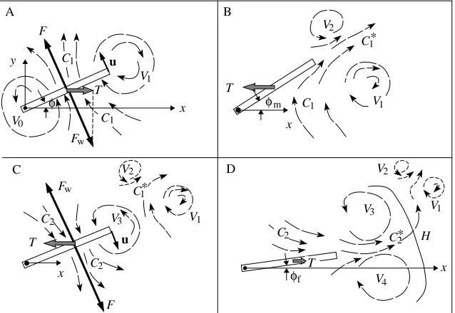
We can interpret the flow-visualization pictures (Fig. 7) given this concept of mutual induction. In the initial flip (Figs 7B, 8A), the tip of the tail moves with tip velocity vector
u. The tail fin applies a force, F, that sets up the current
element, C1. The tail experiences the reaction force, Fw. Its x-component, T, causes the drag on the body (negative thrust). The current element C1induces the vortex V0near the axis of rotation and the vortex V1behind the trailing edge.
After the tail fin has come to a sudden stop at its maximum deflection, φm(Figs 7C, 8B), the fluid current, C1, driven by its own inertia, pushes against the fin. This action causes a thrust force, T, that gradually builds to the plateau shown in Fig. 4. T pushes the fin in the intended swimming direction (negative x). Since the fin is held fixed at the deflection angle,
φm, the fluid current must change direction. This acceleration causes additional thrust. The redirected flow (labeled C1*) and the vortex V1are pushed slightly to the side. As C1* emerges at the trailing edge of the fin, the vortex V2is induced, and the ‘structure’ of a vortex pair (V1and V2) and its intervening fluid current C1* becomes apparent. Such vortex pairs may persist for some time, drifting slowly across the tank. In an ideal frictionless fluid, these vortices would coast along indefinitely without decay as required by Kelvin’s law of conservation of vorticity.
The thrust in the plateau is the reaction force required to change the momentum from C1to C1*. The thrust lasts until the ‘structure’ has oriented itself so that the remainder of the current, C1*, still in the vicinity of the tail, flows parallel to the tail fin. The gradual decrease of the thrust force plateau as a function of τrin Fig. 4 indicates how the current C1* in time loses its velocity component perpendicular to the tail. However, the motion in the water is not spent. What remains of current C1* increases the relative velocity between the tail and the fluid during the return flip and causes the thrust spike seen in Fig. 4. The return stroke is not captured in Fig. 7; it occurs between frames C and D. However, in Fig. 8C, we illustrate our thoughts on the appearance of flow structures in the middle of the return stroke. The tail tip moves back towards the rest position as indicated by the velocity vector,
A
B
C
D
E
F
V
3V
4C
2*
V
3V
4V
1C
1*
V
2V
0V
1V
1C
1*
[image:8.609.52.556.70.677.2]V
2Fig. 7. Photographs showing the flow field around the simulated fish tail, visualized using aluminum filings. The camera is mounted at a slight angle with respect to the rotation axis to reduce reflection. During frame A, the tail is stationary, while during frame B the tail moves sideways as indicated on Fig. 2. After stopping momentarily (C), the tail returns to its initial position (D). A pair of vortices with a current flowing away from the tail are shown in E and F. The photographs were taken at 3 Hz with an exposure time of 0.25 s as indicated on Fig. 4. V0, vortex created by forebody; V1,
reaction is the thrust T. As long as the initial current C1* is not entirely spent when the return stroke occurs, the relative velocity between the water and the tail must be larger than during the initial stroke. Therefore, the thrust during the return stroke must be larger than the drag of the initial stroke. The inertia in the water, set into motion by the initial stroke, causes the unequal drag and thrust in the initial and return phases. This concurs with the momentum-reversal model, where the flow set up by the initial stroke enhances the thrust extracted by the return stroke.
Fig. 8D corresponds to Fig. 7D. It illustrates the flow as the tail tip reaches its final fixed position. Again, the fluid current C2, set up by the return stroke, runs into an obstacle and changes direction to become the current C2*. The acceleration required to change C2into C2* induces a force onto the tail that contributes to the thrust. C2 induces the vortices V3 and V4. Since the final tail angle, φf, is larger than zero, there is a residual drag force (Fig. 7F). If the flow was visualized using dye rather than particles, we would probably see the outlines of vortices V3and V4and the head H of a ‘mushroom cloud’ marking the leading edge of current element C2*. Such views of similar vortex patterns are seen in studies by Rosen (1959) and Maxworthy (1979).
We reiterate that the forces measured in this stationary tail simulation give a quantitative account of the propulsive forces generated during the very first moments of a fish fast-start, when the fish has not yet moved relative to the water. Our results have only qualitative significance for the later phases of the motion.
Quantitative analysis of half-flips
It is possible to extract a value for tail force F since it is related to the negative thrust precursor as T=−Fsinφ. For a maximum negative precursor, T≈−0.03 N, found at φ=35 °:
F = −T/sin35 °≈0.05 N . (13)
This calculation can be compared with the thrust forces generated during steady swimming. The thrust force as calculated in Ahlborn et al. (1991; equation 4) is:
T = 25ρh A3f2, (14)
where ρ is the density of water, h is the section height, A=Lsinφmis the swing amplitude of the tail tip and f=1/τis the tail frequency. With ρ=1 g cm−3, h=15.0 cm, L=5.0 cm and
φm=35 °,
A = Lsinφm = 2.9 cm . (15)
A trapezoidal tail flip curve resulting from these experiments has no unique frequency. However, an upper and lower bound can be calculated. The lowest frequency, fmin, is found from the time τ1/2during which the tail tip makes one excursion and returns to the original position. Fig. 4 shows τ1/2=1 s, which yields fmin=0.5 Hz. The highest frequency, fmax, is defined by the time, τo, that it takes to reach the maximum deflection. With
τo=τ*/4≈0.2 s, where τ* is the time for one full tail beat, then
fmax=1/τ*≈1.3 Hz. When these values are entered into equation 14, a lower limit for the thrust can be derived using the same dimensions as in equation 14:
Tmin≈25ρh A3×0.52 = 0.022 N , (16) and an upper limit:
Tmax≈25ρh A3×1.252 = 0.13 N . (17) The measured thrust of 0.05 N, given by equation 13, falls into the middle of the range set by the momentum-reversal model. The Reynolds number used here, based on tail tip velocity, u, and tail length, L, is typically approximately 5000. The Reynolds number of a swimming fish would be approximately five times larger. However, in the Reynolds number range 5000–50 000, structures in the flow do not change significantly. Therefore, our results will still reveal qualitative aspects of fluid motions around fish tails. The C
V
V T F
F
x y
φ V
T
C
C
V
T
C V
V
C
u
T
V
V
x V
φm
A B
C D
V
F
u
F x
x
C
C
V C
C H
φf
1 1
1 1
0
2
1
1 1
2
3 1
1
2 2
3 w
w
2
2 2
4
*
[image:9.609.248.567.74.294.2]* *
Fig. 8. Schematic diagram illustrating the flow contours of B–E on Fig. 7. x and y are the reference axes; F is the force of the tail acting on the water and Fwis the reaction force of the water acting on
the tail; T is the thrust force along the x-axis; V0–V4
refer to vortices produced sequentially by the tail movements; C1 and C2and C1* and C2* refer to
frequencies were selected to optimize the data acquisition from the apparatus and, as a result, the period for the tail cycle is longer than might be expected from real fish. The principle difference is that a real tail is a three-dimensional structure, whereas we have an approximation of a two-dimensional tail. The tail beat frequency used here was 0.5–1.25 Hz, whereas measurements from fish indicate cruise frequencies of approximately 3–7 Hz (Bainbridge, 1960; Altringham and Johnston, 1990; Rome and Swank, 1992) and much higher values during burst swimming (Harper and Blake, 1990). Using a lower tail beat frequency affects the hydrodynamics, but the qualitative aspects of the fluid movement are similar.
Discussion
Measurements of the thrust and impulse produced by a simulated fish tail reveal distinctive phases of motion relevant to fish fast-starts: (i) a negative precursor, (ii) an impulse-generating phase in which the sideways flow is deflected towards the rear, and (iii) a maximum thrust phase where the direction of momentum is inverted. Phases ii and iii produce active wakes with vortices that turn in the opposite sense to the von Kármán vortices in the wake of a dragged object.
Fast-starts resembling the C-starts defined by Weihs (1973) involve a flip and return motion. The tail bends sideways to an angle φand then returns to the straight position. The gravity-driven tail-flip apparatus of Ahlborn et al. (1991) simulated this motion as a continuous process, where the return flip followed the initial stroke without delay. The momentum-reversal model also assumes that no time elapses between the production and destruction of the first vortex. However, when fish swim, these simple kinematics may be modified: fish can momentarily hold their tail in a bent position before they straighten again (Harper and Blake, 1991). A pause of duration
τroccurs between the initial and return strokes. To assess the physiological significance of these kinematics, we redesigned the tail-flip apparatus so that the tail would execute a flip and return of arbitrary deflection angle φmseparated by a resting interval τr. By varying the resting interval, we could investigate the kinematic effects of each phase of the motion. The device also enabled measurement of the time-resolved propulsion forces, Fx(t), and the accumulated impulse, J(t)=∫Fx(t)dt. The results showed that the impulse has a maximum value for a particular resting interval, τr.
The results also show that impulse optimization is affected by two factors: (i) a delay of τr=0.9 s between the initial and return stroke yields maximum thrust for our apparatus, and (ii) tails of intermediate flexibility produce larger impulses than either stiff or very flexible tails. Fig. 6 shows a clearly discernible difference in the peak impulse when tails of varying stiffness are used. The tail of medium flexibility generated the most thrust. In these experiments, we also recorded the current, j, and the voltage, Vm, applied to the tail deflection motor to calculate the power input, P=jVm.All three tails had the same power consumption curve, P(t) (results not shown). Therefore,
differences in momentum and impulse must have arisen from hydrodynamic differences.
The stiffness and shapes of the model tails do not accurately reflect those of real fish. True fish tails are probably capable of actively ‘self-cambering’ (McCutcheon, 1970) to maximize thrust and efficiency during the tail beat. Although tails of varying flexibility are used in the present experiments, they still do not behave like real tails. The active, dynamic changes in tail shape and stiffness of live fish are not, as yet, well understood. The use of very stiff and very flexible fins here is an attempt to simplify the dynamics of the tail movements and to show that the stiffness of the tail is a significant parameter for efficient aquatic propulsion. To further simplify the flow visualizations and analysis, a two-dimensional tail model was used; a straight edge extending from above the surface of the water to just above the bottom of the tank (Fig. 1). Real fish tails will have complex, three-dimensional motion and will be subject to considerable circulation around their upper and lower tips.
A simple extension of the momentum-reversal model shows that the expended energy may be minimized at constant thrust if the vortex produced initially is reversed in direction and a specific value for the final angular velocity is achieved. The calculations were carried out for a simplified vortex model. However, the energy minimum arises from the form of the equations; the thrust force arises from differences in angular momenta, while the energy increases in proportion to the sum of the squares. Therefore, the momentum-reversal model shows that energy minimization should also be possible in more realistic models.
An interesting effect emerged from the kinematically similar motion of the initial and return strokes; the drag and thrust forces are unequal. We attribute this effect to the inertia in the fluid ‘structures’ initially induced. The residual motion of the water after the initial stroke increases the relative velocity between the tail and water during the return stroke. The return stroke, therefore, must invert the momentum that was induced by the initial stroke. This concurs with the momentum-reversal model of fish propulsion (Ahlborn et al. 1991). The model predicts that one sweep of the tail fin generates (angular) momentum that enhances thrust generation by the return phase of the tail beat.
Although the model fish tail used here does not closely resemble a real fish tail, we believe that the four phases of motion of the tail flips shown here should also be found for real swimming fish. For example, a specific prediction can be made from the small negative impulse, late in phase 1 (Fig. 4), at the maximum excursion of the tail. This suggests that the tail should maintain a positive angle for a certain period τrand flip quickly when the tail is moving laterally to reduce the effect of the negative impulse. This prediction was also derived from Lighthill’s (1971) analysis and was noted in two previous studies on swimming fish (Lighthill, 1971; Wardle and Reid, 1977).
design of the apparatus and the computer program. The extensive comments by the referees are also greatfully acknowledged.
List of symbols
A amplitude of deflection of the tail tip As amplitude of spring extension
B magnetic field
C1, C2 first and second current elements
C* redirected current element dm mass element in the fluid
ΣE total kinetic energy invested
Ei rotational kinetic energy of vortex V1
Ef rotational kinetic energy remaining in the water after torque Γhas acted on V1
Emin minimum energy expenditure
Ep accumulated potential energy
f tail flip frequency
fmin minimum tail flip frequency
fmax maximum tail flip frequency
F force of the tail acting on the water Fr centrifugal force
Fw reaction force of water acting on the tail
Fx thrust force component in x-direction
Fx,ΣEmin thrust force delivered when energy expenditure is minumum
Fy thrust component in y-direction g gravitational acceleration
Gi angular momentum of the vortex created by the first sideways motion
Gf angular momentum after the tail has interacted with the vortex
h submerged height of model tail H borders of ‘mushroom cloud’ Ii moment of inertia of initial vortex
Ii′ moment of inertia associated with total initial kinetic energy
If moment of inertia of the final vortex
If′ factor giving the correct total kinetic energy with average angular velocity ωf
j electric current
J total impulse for time interval ∆t J(t) impulse accumulated at time t
K entrainment constant
k spring constant
L length of the model tail
m mass of an object
P power input to motor
∇p pressure gradient
r distance from centre of rotation of the vortex ro local radius of curvature
t time measured from beginning of tail flip
∆t time during which torque Γis applied T thrust force acting on hinge (=Fx)
Tmin, Tmax lower and upper limits of thrust force
U flow velocity
u average tail tip velocity
u tail tip velocity vector v velocity of an object
V vortex
V0 vortex created by forebody
V1 vortex created by first sideways flip
V2–V4 subsequent vortices produced sequentially
Vm voltage
x, y, z spatial coordinates
x direction of fluid flow relative to tail
x1 moment arm of force Fygenerating the vortex V1
y2 moment arm of force Fxwhich stops or reverses vortex V1
Ε electric field
Γ torque changing vortex V1into vortex V2
φ tail angle with respect to the x-axis
φm maximum tail deflection
φf final tail deflection angle
ρ water density
τ time interval of tail flip
τc closing (return) time of the tail
τo opening (excursion) time of the tail
τr resting time of the tail
τ1/2 time for one excursion of the tail and return to original position
τ* time for one full tail beat
ω angular velocity of vortex
ωi average angular velocity of vortex V1
ωf average angular velocity after Fxacts on vortex
ωi,min initial angular velocity at minimum energy expenditure
ωf,min final angular velocity at minimum energy expenditure
ξ line of vorticity
References
AHLBORN, B., HARPER, D. G., BLAKE, R. W., AHLBORN, D. ANDCAM, M. (1991). Fish without footprints. J. theor. Biol. 148, 521–533. ALEXANDER, R. MCN. (1987). Bending of cylindrical animals with
helical fibres in their skin or cuticle. J. theor. Biol. 124, 97–110. ALTRINGHAM, J. D. ANDJOHNSTON, I. A. (1990). Modelling muscle
power output in a swimming fish. J. exp. Biol. 148, 395–402. BAINBRIDGE, R. (1960). Speed, amplitude and tail-beat frequency of
swimming fish. J. exp. Biol. 37, 129–153.
CHENG, J. Y. ANDBLICKHAN, R. (1994). Bending moment distribution
along swimming fish. J. theor. Biol. 168, 337–348.
FREIMUTH, P. (1989). Vortex pattern of dynamic separation. In Encyclopedia of Fluid Mechanics, vol. 8, p. 391. New York: McGraw Hill.
FRITH, H. R. AND BLAKE, R. W. (1991). Mechanics of the startle response in the northern pike Esox lucius. Can. J. Zool. 69, 2831–2839.
HARPER, D. G. ANDBLAKE, R. W. (1990). Fast-starts of rainbow trout, Salmo gairdneri and northern pike Esox lucius during escapes. J. exp. Biol. 148, 128–155.
HARPER, D. G. ANDBLAKE, R. W. (1991). Prey capture and the
fast-start performance of northern pike Esox lucius during escapes. J. exp. Biol. 155, 175–192.
LIGHTHILL, M. J. (1971). Large-amplitude elongated-body theory of fish locomotion. Proc. R. Soc. Lond. B 179, 125–138.
MAXWORTHY, T. (1979). Experiments on the Weis-Fogh mechanism of lift generation by hovering flight. J. Fluid Mech. 93, 47–63 MCCUTCHEON, C. W. (1970). The trout tail fin: a self-cambering
hydrofoil. J. Biomech. 3, 271–281.
MCCUTCHEON, C. W. (1977). Froude propulsive efficiency of a small fish measured by wake visualization. In Scale Effects in Animal Locomotion (ed. T. J. Pedley), pp. 339–363. London: Academic Press.
PRANDTL, L. AND TIETJENS, O. G. (1934). Applied Hydro and Aeromechanics. New York: Dover Books. 311pp.
ROME, L. C. ANDSWANK, D. (1992). The influence of temperature on power output of scup red muscle during cyclical length changes. J. exp. Biol. 171, 261–281.
ROSEN, M. W. (1959). Water flow about a swimming fish. United States Naval Ordinance Test Station Technical Publication 2298, 1–96. WARDLE, C. S. AND REID, A. (1977). The application of the
large-amplitude elongated body theory to measure swimming power in fish. In Fisheries Mathematics (ed. J. H. Steele), pp. 171–191. New York: Academic Press.
WEIHS, D. (1973). The mechanism of rapid starting of slender fish. Biorheology 10, 343–350.
YATES, G. T. (1983). Hydromechanics of body and caudal fin