Implementing and analysing the fast marching method

University of Twente

Bachelor Thesis

Implementing and Analysing the Fast

Marching Method

Author:

Dieuwertje Alblas

Supervisor:

Yoeri Boink MSc.

Contents

1 Introduction 2

2 Fast marching method 3

2.1 Outline of the algorithm . . . 3 2.2 Algorithm details . . . 4

3 Implementation 6

3.1 Expansion of the algorithm . . . 8

4 Analysis 9

4.1 Mathematical analysis . . . 9 4.2 Complexity . . . 11 4.3 Expansion of the algorithm . . . 12

5 Application 14

5.1 Blood vessel segmentation . . . 14 5.2 Route planning . . . 16

1

Introduction

The fast marching method is an algorithm that is developed in the 1990’s by J.A. Sethian (1996a). The method is similar to Dijkstra’s algorithm, that is used for finding optimal paths in a graph (Dijkstra, 1959). The goal of the fast marching method is to solve a discretised version of the Eikonal equation on a uniformly sized spatial grid. This solution has the form of a fictional arrival time for each point of the grid, originating from a point chosen beforehand. To accomplish this, a speed function is defined on each of the points of the grid. From the chosen starting point, this speed function is used to calculate the arrival times of the other points in the grid iteratively, point by point.

Besides solving the Eikonal equation on a 2D uniformly sized spatial grid, the fast marching method has been implemented for spherical coordinates by Alkhalifah and Fomel (2001). Sun et al. (1998) looked into solving the Eikonal equation numerically on an unstructured grid. It has also been used for calculating 3D travelling time by Sethian and Popovici (1999).

The fast marching method has a lot of applications. For example, in Deschamps and Cohen (2002), the fast marching algorithm is used for reconstruction of tubular objects. It can also be used for shortest path planning, as done in Garrido et al. (2006). Here, a more efficient version of the fast marching method was used to plan a route for a robot, without running into obstacles. In this report, the fast marching algorithm will be used to perform blood vessel segmentation. The algorithm will also be used as an alternative form of route planning.

Concluding, solutions of the Eikonal equation are of great use within many fields of research. However, computing these solutions analytically would be very time-consuming. Therefore, an implementation of the fast marching method is desirable. An implementation in_matlabalready exists1_{, as well as an implementation partly written in Python and C++}2_{. However, there is no}

implementation written entirely in Python yet. A Python implementation could be useful, because not every researcher understands _matlab or C++. Furthermore, to use Python, no expensive licences are necessary, which makes the Python code more accessible than thematlab implemen-tation. The goal is to build an implementation of the fast marching method in Python that is at least as fast as the existing matlabimplementation.

In this report, the fast marching method will be briefly explained. After that, the details of the implementation will be discussed, as well as the mathematical accuracy and the complexity. We will also look into improving the efficiency of the algorithm by adding more than one grid point per iteration. Finally, we will discuss two different applications of the fast marching method.

1_{Toolbox made by Gabriel Peyre, https://nl.mathworks.com/matlabcentral/fileexchange/}

6110-toolbox-fast-marching

2

Fast marching method

You can think of the fast marching method as an oil slick, that is dropped on an uneven surface. This slick will spread over the surface. The way this slick will spread, depends on different factors, for instance the smoothness of the surface at each location. Imagine we are interested in the propagation of the front of the oil slick, in particular the time it takes before the front reaches each point on the surface. In essence, this is the goal of the fast marching method.

To put this idea in a mathematical framework, we consider a spreading closed curve Γ on a surface. For generality, this surface has a dimension of two or higher. The way this curve spreads depends on the speed function F(~x) defined on the surface. We are interested in how the curve is spreading over the surface over time. To describe the position of the spreading curve Γ, it is possible to define an arrival time functionT(~x) as it crosses each point~x. IfF(~x)>0 ∀~xon the surface, this functionT(~x) satisfies the Eikonal equation:

|∇T|F = 1 (1)

This notation is called the boundary value formulation. This equation can be solved numerically using the fast marching method. However, if F(~x) < 0 for some points ~x, the fast marching method cannot be used to solve for T(~x). This situation occurs, because a point can be visited more than once by the curve, hence T(~x) can have more than one value. In this case, the initial value formulation is used. More information about situations where F(~x) < 0 can be found in Sethian (1996a). In this report, there will only be situations whereF(~x)>0, so only the boundary value formulation will be used.

2.1

Outline of the algorithm

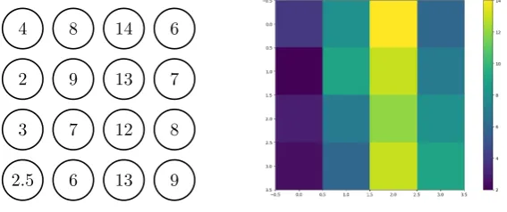
In the previous paragraph it was described that the goal is to find a functionT(~x) to describe the propagation of the initial front over time. This is a continuous problem. To find this function using the fast marching method, the problem has to be transformed into a discrete problem. There-fore, the domain has to be discretized into a uniformly sized spatial grid. The continuous speed functionF(~x) becomes a discrete function that is defined on every point of the grid, with abuse of notation now denoted byFi,j. As an example, a speed function on a 4x4 grid is shown in figure 1.

12 8 7 3 13 14 13 6 7 6 9 9 8 2.5 2 4

Figure 1: Possible speed functionFi,j on 4x4 grid

To initiate the fast marching algorithm, an initial front needs to be defined. This is usually done by choosing a single starting point (i, j) on the grid, and define the functionTi,j to be zero

there. Also, the points on the grid are divided into three sets: far, known andneighbours. The starting point is an element of known, sinceTi,j has a known value there. The points next to the

in the set known.

Known

Neighbours

Far

Figure 2: The sets known, neighbour and far on the spatial grid.

The next step in the fast marching method is calculating the values ofTi,jfor the newly added

neighbours and updating them if necessary. A more profound description of the way these values are calculated and updated can be found in section 2.2. The neighbour that has the smallest calculated value ofTi,j is added to the set known. This process takes place iteratively, until either

the given end point is in the set known, or all the grid points are in the set known. The process of the fast marching method is described in figure 3.

Calculate arrival times of newly added neighbours

Find the smallest value of neighbours

Add coordinate of the smallest value to known

Move new adjacent points from far to neighbour If end point∈/ known,

or∃(i, j)∈/ known

Figure 3: Flowchart of the fast marching algorithm

2.2

Algorithm details

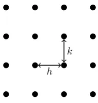
Now the outline and goals of the algorithm are clear, it will be discussed in more detail. For calculating the arrival times of the newly added neighbours, Sethian (1996a) uses a time scheme with spatial derivatives. To clarify the definition of the spatial derivative, take a look at figure 4. In this picture we see a uniformly sized spatial grid.

h k

Figure 4: 4x4 spatial grid withx-spacinghandy-spacingk.

Suppose we are interested in a value of a function T(x, y) on this spatial grid. Two types of spatial derivative operators are defined as follows:

D+xT =T(x+h, y)−T(x, y)

h (2)

D−xT =T(x, y)−T(x−h, y)

The operator (2) is called the forwards operator, because it uses the information ofT(x+h, y) to find a value for T(x, y). This operator propagates from right to left. Similarly, (3) is called the backward operator and propagates from left to right.

A discrete version of this difference operator is used to calculate the values of Ti,j, using the

speed functionFi,j at the specific point. To do so, the following scheme is used:

_max(D−x i,jT,−D

+x i,jT,0)

2

+max(D_i,j−yT,−D+_i,jyT,0)2

12

= 1

Fi,j

This can be interpreted as follows, whereTi,j is the arrival time at location (i, j):

max(Ti,j−Ti−1,j, Ti,j−Ti+1,j,0)2

+max(Ti,j−Ti,j−1, Ti,j−Ti,j+1,0)2

12

= 1

Fi,j

Only the values ofTi,jof points (i, j) that are elements of the set known can be used for calculating

the values of the neighbours. To calculate the value forTi,j we use the method presented in R.

Kimmel and J.A. Sethian (1996):

a= min(Ti−1,j, Ti+1,j)

b= min(Ti,j−1, Ti,j+1)

Now solve the quadratic equation forTi,j as follows:

If 1

Fi,j

>|a−b|, thenTi,j=

a+b+

r

2_F1

i,j

2

−(a−b)2

2 . (4)

Otherwise, letTi,j=

₁

Fi,j

2

+ min(a, b). (5)

These calculations are only done on the neighbours of the newly added point. If the value of a point (i, j)∈neighbours has been calculated before, the value found before will be updated, only if the newly found value is smaller.

3

Implementation

In this paragraph the implementation of the fast marching algorithm will be explained. The goal is to have speed function matrixFi,j as input, together with a start point and an end point. The

iterative process of calculating new arrival times will continue, until the given end point is an element of the set of known points. The output of the implementation will be a matrix the same size asFi,j containing all the known arrival timesTi,j. This will be the discretized version of the

aforementioned function of interestT(x, y).

The implementation is object based, so each object has its own functions that can be applied on it. As a side effect, this will give a better overview of all the separate parts of the algorithm. All the objects will be discussed in the following sections.

Status

This object is a matrix the size of Fi,j. It keeps track of the points in each of the sets known,

neighbours and far. Initially, this is a matrix containing only -1 values. This value means that the point to which this value is assigned is an element of the set far. Similarly, 0 means the point is a neighbour and 1 means the point is known.

Status has a few different functions that are defined on it:

• n2k is short for neighbour to known. It adds the point it is given as an input to the set known by changing its value in the matrix to 1.

• f2n, short for far to neighbour is called by n2k. It adds the adjacent points of the newly added point to the set neighbours by changing the status of the point from -1 to 0.

Times

This object is also a matrix the same size asFi,j. It keeps track of the values ofTi,j at different

points. When it is constructed, the value of the start point in this matrix is set to 0. The values of the remaining points are initially set at infinity.

Similar to the object status, the times class also has different functions that can be applied on the object:

• The first function isaddtime, that simply adds a calculated value ofTi,j to the given point

of the times matrix.

• The second function iscalctime. This function calculates the time at a given point, with the method given in 2.2. It returnsTi,j as well as the coordinates of the point (i, j).

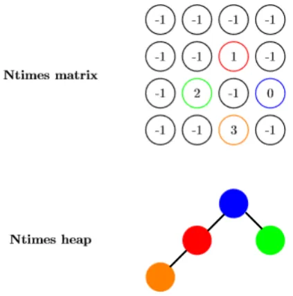
Ntimes

The class Ntimes consists of two objects. One of the objects is a heap, that contains and organises the calculatedTi,j of the neighbours. Besides the calculated value of each point in the neighbours

set, it also contains the coordinates of each calculated value. The form of the elements is a three dimensional vector, with the first tuple being the calculated arrival time, and the second and third tuple the coordinates of the point. The smallest value of this heap will be added to the set known each iteration. As stated before in 2.2, finding the minimum value is very efficient due to the min heap structure. The second object that is a part of the Ntimes class is a matrix the same size as

Fi,j. This matrix keeps track of which points already have a calculated value and where they are

located in the heap. In figure 5 the connection between the heap and matrix will be clarified.

Also on this object, several functions are defined:

• The second functiondelete is similar toinsert, but this function deletes a given entry from the heap, while maintaining the desired structure. It also keeps the matrix up-to-date with the correct entries. For detailed descriptions of both functionsinsert anddelete, please refer to Forsythe (1964).

• The third function checkdouble calls both the functions insert and delete. It has the calcu-lated time and the coordinates of the grid point as input. It checks for the given grid point if another value was already calculated for the same point. To do so, it uses the matrix. If the value in the matrix for this coordinate is equal to -1, there is no value for this coordinate yet. The function will call the function insert to simply add the new value to the heap. If the value in the matrix of the given grid point is not equal to -1, it means that there was already a value calculated. The value in the matrix will be used to trace back the existing value in the heap. Then it will be checked if the newly calculated value is smaller than the old value. If that is the case,delete will be called on the old value and insert will be called on the new value. If the new value is larger than the old value, the new value will be ignored and the old value will remain in the heap.

calctime on newly added neighbours

checkdouble on newly calculated values, adds values to heap

addtimeon smallest value in heap

n2k on smallest value in heap

f2n on smallest value in heap If end point ∈/ known

Figure 6: Flowchart of the implementation

The collaboration between the different objects in the code is depicted in figure 6. When it is compared to figure 3, we see the same steps, but now put in the framework of the functions defined above.

3.1

Expansion of the algorithm

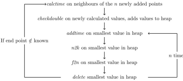
As stated in the introduction, we will look into improving the speed of the algorithm by adding more than one point per iteration. Here, this is done using the functions of the implementation described above. To accomplish this, the current implementation needs a few changes. For ex-ample, the smallest values of the heap are added to a list. The values of Ti,j for the neighbours

of the points in this list are calculated at the beginning of the next iteration. The flowchart in figure 7 describes the implementation wherenpoints are added per iteration. The complexity and accuracy of this implementation will be assessed in section 4.3.

calctime on neighbours of thennewly added points

checkdouble on newly calculated values, adds values to heap

addtime on smallest value in heap

n2k on smallest value in heap

f2non smallest value in heap

delete smallest value in heap If end point∈/ known

ntimes

4

Analysis

4.1

Mathematical analysis

The fast marching method is a quick method to solve the Eikonal equation numerically. However, at the core it is relatively inaccurate. In Sun et al. (2017), the fast marching method is combined with wavefront construction. This is another, less efficient, method that can solve the Eikonal equation numerically and has a more accurate solution. In this paragraph we will look into the accuracy of the found solutionTi,j.

To be able to find the error in the fast marching method, a uniformly spaced grid has been used, with Fi,j equal to 1 on the entire grid. Now it is possible to use the distance between the

starting point and each point of the grid to calculate the actual arrival times of each point. Since the speed is equal to 1, the arrival time at each point will be equal to the computed distance from the starting point. This will be the arrival time we will compareTi,j to.

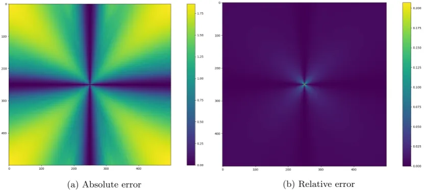
Figure 8a shows the absolute difference between Ti,j and the exact value. What immediately

stands out is that the error on the diagonal axes is much higher than on the horizontal and vertical axis. Another striking feature is that the error increases to the outer diagonal parts of the image. However, the value of the arrival time increases much faster than the error. Therefore, the relative error has a much lower value than in the core of the image.

(a) Absolute error (b) Relative error

Figure 8: Errors of fast marching method

The error in the fast marching method is due to discretization. Close to the starting point, the absolute errors are easy to explain. Farther away it will become an accumulation of many small errors and therefore hard to keep track of what exactly went wrong. Because the relative error is small far away from the starting point, we will analyse the part close to it.

In figure 9a we can see that the absolute error of the fast marching method is 0 on the horizon-tal and vertical axis. That is due to the fact that the front propagates accurately in this direction. Already in the first diagonal neighbours of the starting point, we see a relative error of approxi-mately 0.3. This is the case, because the distance, and therefore also the arrival time, between the starting point and its diagonal is equal to√2. However, the fast marching method will first add the direct neighbours of the starting point to the set known, because they have a smaller value of

Ti,j. Therefore, the front first propagates to the direct neighbours of the starting point, that will

(a) Absolute error (b) Relative error

Figure 9: Errors of the fast marching method, zoomed in

the edges of the diamond, as we can already observe in the first diagonal neighbours the front encounters. The diamond that has arisen after 1 time step, has to travel a distance of

√

2

2 to arrive

at the diagonal neighbour. Together, this accounts forTi,jof 1 +

√

2

2 ≈1.71 for the fast marching

method, versus the actual time√2≈1.41. This explains the error of 0.3. In the remainder of the point, the same phenomenon occurs, but it is harder to keep track of the exact error, sinceTi,jis

based on a value ofTi,j that already was inaccurate.

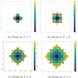
As already stated, the front propagates in a diamond shape, this can be seen in figure 10. This is due to the discretization of the problem. In the continuous version of the problem, the front would have propagated in the shape of a circle.

(a) Front atT = 1 (b) Front atT = 2

(c) Front atT = 3 (d) Front atT = 4

4.2

Complexity

The complexity of the algorithm is assessed here. This offers important information for the run time of the algorithm in relation to the size of the input. The complexity is assessed both analyt-ically and numeranalyt-ically.

The complexity of the fast marching algorithm isO(nlog(n)), wheren is the number of grid points of the input (Sethian, 1996a). For the implementation, the complexity of the used functions in each iteration will be analysed one by one.

• Calctimehas to calculate the times of three new neighbours worst case, with an exception in the first iteration of the algorithm, where the values of four neighbours have to be calculated. However, if the number of grid points tends to ∞, only 1 neighbour is added per iteration. We will focus on what happens for big numbers of grid points. Within this function, a constant number of arithmetic operations have to be performed.

• Checkdouble has to check if one of the values was already calculated. To do so, it has to check the matrix if the given point already has a value in the heap. Checking if there is already an existing value in the heap are a constant number of operations. The bottleneck in the efficiency is replacing a value in the heap. This is a worst case scenario, since now bothdelete andinsert have to be called. Both have an efficiency ofO(logn), withnthe size of the heap (Forsythe, 1964).3

• Finding the minimum of the heap only takes one operation. Calling delete to get rid of this entry has a complexity of O(logn), with againnthe size of the heap.

• Changing the status of the newly added point and the neighbours will take four operations worst case. When the number of grid points tends to ∞, this will only take two operations.

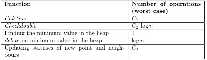
As we can see, there are some functions that take a constant number of operations. These constants are denoted byCi,i= 1,2,3 in table 1.

Function Number of operations

(worst case)

Calctime C1

Checkdouble C2 logn

Finding the minimum value in the heap 1

delete on minimum value in the heap logn

Updating statuses of new point and neigh-bours

C3

Table 1: Number of operations per function

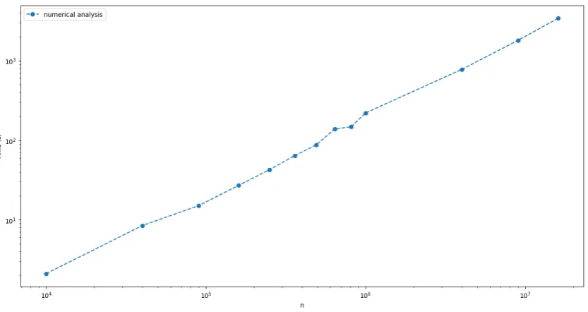
Concluding, the total number of operations per iteration is A1+A2logncomplexity per

iter-ation. Worst case,niterations are necessary to reach the end point. Therefore, the total number of operations is equal to A1n+A2nlogn. The values of A1 and A2 differ per implementation.

In this implementation,A1≈30 and A2≈7. Therefore, A1nwill grow faster thanA2nlogn for

relatively small values ofn. This phenomenon will cause the numerical analysis to appear linear, which can also be seen in figure 11.

Besides an analytical assessment of the complexity, the complexity was also analysed numeri-cally. To do so, a square spatial grid was used, with a constantFi,j defined on it. The size of the

spatial grid was increased. The time needed to perform the fast marching algorithm on each of the grids was recorded. The results of this experiment can be seen in figure 11.

Figure 11: Plot of the numerical complexity of the fast marching method

4.3

Expansion of the algorithm

The accuracy and efficiency of the implementation presented in section 4.3 will be assessed here.

The accuracy of the implementation addingnpoints per iteration will be compared to the fast marching method adding one point per iteration. Addingnpoints per iteration can cause a bigger inaccuracy in certain situations. The reason why the fast marching method works, is because each iteration only the smallest value is added. The main idea behind this is that the smallest value ofTi,j cannot be affected by the bigger values. In the original algorithm, the neighbours are

updated each iteration, because there may be a smaller arrival time via the newly added point. This causes trouble when we add the n smallest points, where some of these points are close together. Because maybe, when updating the times of the neighbours, a smaller value for Ti,j

could have been found. This phenomenon will increase the error of the algorithm. This can be seen in figure 12b. In the speed function shown in figure 12a, there is a sharp change in velocity. The fast marching method adding one point per iteration is compared to adding two points per iteration. The relative difference between these methods can be seen in figure 12b.

(a)Fi,j (b) Relative difference

figure 7, we perform the same operations, but do a loop over the last four. Among these four, we have to call the function delete, that is O(logN) worst case, with N the size of the heap. Also some constant number of operations have to be performed within this loop. This adds up to nlogN +C1n operations per iteration, only for the final small loop. In total, this adds up

to nlogN+C1n+C2logN+C3 per iteration. This is approximately the number of operations

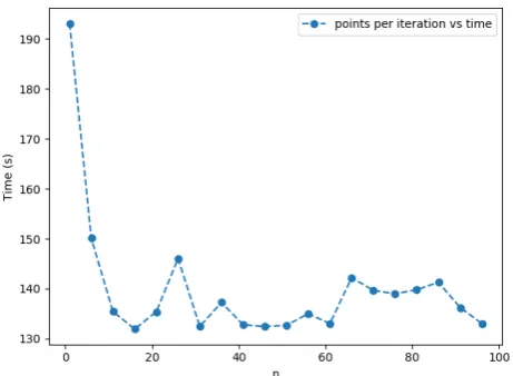
needed forniterations of the normal fast marching algorithm. The only thing that books us time here is not having to recalculate some points, which could cause inaccuracy, as described above. In figure 13 we can see the time needed to complete the fast marching method versus the number of points added per iteration. It is striking that using small values of nbooks quite some time. Increasing the number of added points per iteration aftern≈15 does not book time at all. More research has to be done on this issue.

Figure 13: Time versus number of points added per iteration

It might be useful to use a different data structure to store the values of the neighbours. We have to use a structure that is able to find the n smallest elements efficiently. However, before this will have major impact on the current speed of the algorithm, it is necessary to decrease the number of constant operations, since these contribute considerably more to the run time of the implementation. After this is done, the speed of the implementation can be increased by using a different structure to store the values of the neighbours.

As already stated, the current tree structure is not very efficient to find the smallest n ele-ments. In Frederickson (1993) an O(n) algorithm to find thenth _{smallest element in a min heap}

is presented. However, using this algorithm to find thenth _{smallest elements, would still result in}

anO(n2_{) operation. Hence, this approach would not be very efficient.}

A considerable approach is to use theuntidy priority queue introduced in Yatziv et al. (2006). This storage structure reduces the complexity of the fast marching method to O(k), with k the number of grid points, while maintaining a bounded error. In order to do so, a circular array with

ddiscrete levels ˆTi,i= 1,2, .., dis built. Each entry of the circular array holds a FIFO list, that

contains the calculated values of neighbours within a certain interval. The calculated values are quantized and stored in the correct list in the circular array.

A way of using this structure to add more than one point per iteration, is adding all the points in the list of entry ˆTicontaining the lowest values ofT to known in one iteration. When this approach

5

Application

As already stated in the introduction, the fast marching method has a lot of different applications. Here, we are going to look at two different applications. The first one is a form of blood vessel segmentation. The second one is an alternative form of route planning.

5.1

Blood vessel segmentation

To use the fast marching implementation for blood vessel segmentation, a picture of a blood vessel structure was used as a basis for the speed functionFi,j:

Figure 14: Original image of blood vessel structure4

The speed function is based on the colour of the pixel. It is defined such that a dark pixel results in a higher speed. This means that the speed on the blood vessels will be higher than the speed outside the blood vessels. The maximum value ofFi,j is 1, the minimum is equal to 0.1. In

figure 15 we see figure 14 translated to the speed function matrixFi,j.

Figure 15: Fi,j of original image

Now that Fi,j is known, the fast marching algorithm can be applied. In this specific example,

the start point is located in a blood vessel in the top left part of the image, and the end point is located in a blood vessel in the bottom right part of the image. The functionTi,j can be seen in

figure 16.

Figure 16: Ti,j originating from the top left

Using the matrix Ti,j, the shortest path between the start point and the end point can be

found. This is done using the gradient descent method.5 _{Because the speed was defined to be}

higher over the blood vessels, we can see in figure 17 that the shortest path is running over a blood vessel.

Figure 17: Shortest path from start point to end point on original image

This figure was a very clear picture of a blood vessel structure. However, when a similar pic-ture is not very clear, this is a good and quick technique to find the course of the blood vessels and get a binary picture. This idea can be extended by using the technique from Li and Yezzi (2007). Here, another dimension is added to the input matrixFi,j, using circles of different radii

and measuring the contrast on the inside and outside of the circle. The centers of these circles are on the course of the blood vessel. A high contrast value means that the radius of the circle coincides with the radius of the blood vessel at that point. These contrast values form the newly added dimensionktoFi,j,k. The fast marching method can be applied on this three dimensional

input to also find the radius of the blood vessels at each point, giving a precise segmentation. To be able to use this technique, the current implementation should be adjusted in order to be able to work with three dimensional data.

5.2

Route planning

For the alternative form of route planning, we will use the fast marching method to find the shortest path from Enschede to Maastricht. Therefore, we need a matrixFi,j of the Netherlands.

Figure 18: Fi,j of the Netherlands6

Figure 18 is based on the different types of infrastructure in the Netherlands. The yellow lines are highways, where the speed limit is 130 km/h, with an average speed of 120 km/h. The green lines on the map are roads where the speed limit is 70 km/h The speed is defined to be 0 outside the Netherlands and on waters. In the cities, the speed is 10 km/h. Between the cities and major infrastructures, the speed is defined to be 25 km/h.

In order to find the fastest route between Enschede and Maastricht, the implementation is used with Enschede as a start point and as an end point. In figure 19 the travel times throughout the Netherlands can be seen. From this figure, it becomes clear that the travel time from Enschede to Maastricht is 2.4 hours.

Figure 19: Ti,j starting from Enschede

Again, the gradient descent method is used to find the optimal route. The optimal path from Enschede to Maastricht that was constructed using the fast marching method is compared to the path that is found with Google Maps in figure 20. When we compare the route planned by the fast marching algorithm with the route planned by Google Maps, it is obvious that they are identical. Furthermore, when we look at the estimated travel time, Google Maps estimates a travel time that is somewhere between 2 hours and 20 minutes and 3 hours. The 2.4 hours calculated by the fast marching method lies within the travel time calculated by Google Maps.

(a) Fast marching (b) Google Maps

6

Conclusion and recommendations

As stated in the introduction, the goal was to make an implementation in Python that is at least as fast as thematlabimplementation. Fortunately, the presented Python implementation much faster for greater input than the_matlabimplementation. However, the implementation presented here can still be made more efficient. Primarily, as already discussed in section 4.2, by decreasing the number of arithmetic operations in certain functions.

The implementation that is presented here, only works on a two dimensional image. With a few alterations, the implementation can work with 3D images. It is also possible to use this algorithm for solving the Eikonal equation in more than three dimensions. This could be interesting when using the technique of Li and Yezzi (2007) for segmentation.

The fast marching method is a very quick way to solve the Eikonal equation. However, as already stated in section 4.1, it is relatively inaccurate around the initial point. This can cause trouble in applications where the exact value ofTi,j is very important. For these kinds of

appli-cations, it would be better to use the implementation given in Sun et al. (2017). However, the fast marching method is accurate enough to be applied for segmentation, like in Deschamps and Cohen (2002).

Adding more than one point per iteration, could book us some time. Using this version of the algorithm will not cause major errors, when the underlying speed function Fi,j does not contain

any sharp changes in velocity. Further research has to be done on whether there exists a value of

n that causes optimal efficiency, whether thisn differs per Fi,j, and what this value of n would

be. Also, there can still be looked into a more efficient implementation of adding n points per iteration, as mentioned in section 4.3.

References

Alkhalifah, T. and Fomel, S. (2001). Implementing the fast marching eikonal solver: spherical versus cartesian coordinates. Geophysical Prospecting, 49(2):165–178.

Deschamps, T. and Cohen, L. (2002). Fast extraction of tubular and tree 3d surfaces with front propagation methods. Object recognition supported by user interaction for service robots, 1:1–4.

Dijkstra, E. W. (1959). A note on two problems in connexion with graphs.Numerische mathematik, 1(1):269–271.

Forsythe, G. E. (1964). Algorithms. Commun. ACM, 7(6):347–349.

Frederickson, G. (1993). An optimal algorithm for selection in a min-heap. Information and Computation, 104(2):197 – 214.

Garrido, S., Moreno, L., Abderrahim, M., and Martin, F. (2006). Path planning for mobile robot navigation using voronoi diagram and fast marching. In2006 IEEE/RSJ International Conference on Intelligent Robots and Systems, pages 2376–2381.

Li, H. and Yezzi, A. (2007). Vessels as 4-d curves: Global minimal 4-d paths to extract 3-d tubular surfaces and centerlines. IEEE transactions on medical imaging, 26(9):1213–1223.

R. Kimmel and J.A. Sethian (1996). Fast Marching Methods for Computing Distance Maps and Shortest Paths.

Sethian, J. (1996a). Level Set Methods and Fast Marching Methods. Cambridge University Press.

Sethian, J. A. (1996b). A fast marching level set method for monotonically advancing fronts.

Proceedings of the National Academy of Sciences, 93(4):1591–1595.

Sethian, J. A. and Popovici, A. M. (1999). 3-d traveltime computation using the fast marching method. Geophysics, 64(2):516–523.

Sun, H., Sun, J.-G., Sun, Z.-Q., Han, F.-X., Liu, Z.-Q., Liu, M.-C., Gao, Z.-H., and Shi, X.-L. (2017). Joint 3d traveltime calculation based on fast marching method and wavefront construc-tion. Applied Geophysics, 14(1):56–63.

Sun, Y., Fomel, S., et al. (1998). Fast-marching eikonal solver in the tetragonal coordinates. In

1998 SEG Annual Meeting. Society of Exploration Geophysicists.