Performance analysis of a PAC system with card capacity of c

(1)

1

Faculty of Electrical Engineering,

Mathematics & Computer Science

Performance Analysis of a

PAC System with Card Capacity of

c

Andi Zuhra Wardiyah M.Sc. Thesis

May 2017

Supervisor:

(2)

Abstract

(3)

Acknowledgments

(4)

Production Authorization Card (PAC) systems are widely used in analyzing performance of multi-stage manufacturing systems. The cards are used to control and coordinate materials at each stage of a manufacturing process. Recently, PAC system has been adapted to evalu-ate performance analysis of various systems such as logistics, transportation, warehousing, restaurant, health care, etc. For instance, consider container transportation between ter-minals in a port. This transportation system is known as inter-terminal transportation

(ITT) system. Container delivery in an ITT systems is carried out by vehicles and these vehicles have multiple capacity. In practice, a free vehicle is dispatched as soon as a re-quest is received, but it can carry container up to its capacity. The loading/unloading time at terminals might vary, depending on container types and number of carried containers. When a vehicle is done delivering, it goes back to its pool.

The ITT system described above can be seen as a Production Authorization Card (PAC) system. The requests to move containers is a job in the PAC system, terminals are the network and a fixed number of vehicles are the cards. What is interesting is, instead of serving a single job, cards might serve multiple jobs at a time. This then leads to a question ”What is the best card dispatch scenario such that performance of the system is optimal?”.

1.2 Solution Approach

In this report, we give two approaches for modeling PAC systems. We first provide an exact analysis by assuming exponential service times and inter-arrival times. The states of the system constitute a Markov chain and the stationary distributions of the Markov chain is obtained using the matrix-geometric method. We then provide an approximation model for the case of general distributions of service and inter-arrival time. The approximation model is developed by means of decomposition and is validated using simulation.

1.3 Report Structure

(6)

(7)

2 Literature Review

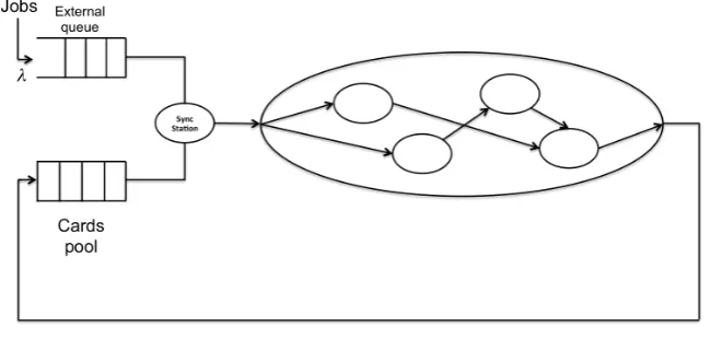
[image:7.595.142.467.248.403.2]

A Production Authorization Card (PAC) system consists of a network of stations with either single or multiple servers, a synchronization station and a finite number of autho-rization cards. In order for a job to be processed, it has to be attached to a card. This process takes place at the synchronization station. Once a job is paired with a card it can proceed to the network. After service completion, the card is released to its buffer.

Figure 1: PAC system

In queuing network terminologie, the PAC system described above is known as a semi-open queuing network (SOQN). SOQN is often used in analyzing performance of manu-facturing and warehousing system ([3], [5], [10], [14]). It is also used in analyzing dine-in restaurant performance [11]. There are several approaches in analyzing SOQN. In [6], Jian & Heragu used the matrix-geometric method. In [10], [11] and [14], the SOQN problem is solved using a decomposition/aggregation approach.

Studies about multi-capacity cards are very limited. To the best of our knowledge, currently [8] is the only study that considered multi-capacity cards. In this report, both matrix-geometric and decomposition approaches are considered in developing the model. At the rest of this section, we provide basic theory used in developing our model.

2.1 Matrix Geometric Method

(8)

recursively. The result of Neuts is described as follows. Consider a Markov process with state space E = (i, j),i≥0 and j is a vector, having infinitesimal generator ˜Q given by

˜ Q=           

B0 A0 B1 A1 A0

A2 A1 A0

A2 A1 A0 · · · A2 A1 · · ·

.. . ...            . (1)

Let π = [π0, π1, π2,· · ·] be the vector of stationary distribution satisfying πQ˜ = 0 and

πe= 1. Then, πk is given by

πk=π0Rk, k ≥0 (2)

with R is the minimum non-negative solution of matrix quadratic equation

A0+A1R+A2R2 = 0. (3)

R can be obtained by successive substitution of

˜

Rk+1 =−(A0+ ˜R2kA2)A−11 (4)

starting with ˜R = 0 and ˜R converges to R.

2.2 Closed Queuing Network

Closed queuing networks (CQN) are often used in analyzing flexible manufacturing systems and computer systems. In general, a closed queuing network is as follows:

• The network consists ofM stations numbered as j = 1,2,· · · , M.

• A fixed number of N identical jobs circulate around the network.

• Each station is either a single or a multi-server station with expected service time 1/µj,j = 1,· · · , M.

• Upon service completion at station i, job moves with probability pij to station j for

j = 1,2,· · · , M, wherePM

(9)

In case of exponential service times, we have a closed Jackson network. The CQN can be analyzed using exact methods or approximation methods. Exact methods are usually used in analyzing Jackson networks and BCMP networks [2] while approximation methods are widely used in analyzing queuing network with general service time.

In this report, we use the Approximation Mean Value Analysis (AMVA) method devel-oped in [3]. Similar to the mean value analysis, the AMVA method was develdevel-oped based on the arrival theorem. Before providing the AMVA algorithm, we introduce the following notations.

• n : number of jobs in the network

• pj(k|n) : marginal probability of k jobs at station j given n jobs in the network

• T Hj(n) : throughput rate to stationj

• Wj(n) : waiting time at station j

• Sj : service time at station j

• S_jrem : remaining service time at station j

• cj : number of servers at stationj

• Lq_j(n) : queue length at station j

• pb_j(n) : probability all servers at station j are busy

• Vj : visit ratio at station j

• µj : service rate at station j

We now provide AMVA algorithm as follows:

1. (Initialization) Set n = 0 and pj(0|0) = 1. Set V0 = 1 and determine other visit ratio’s Vj, j = 1,2,· · · , M.

(10)

3. For j = 0,· · · , M compute

E[Lq_j(n)] =

n−1 X

k=cj+1

(k−cj)p(k|n−1) (5)

E[S_jrem] = cj −1

cj + 1

E[Sj]

cj

+ 2

cj+ 1

1

cj

E[S_j2] 2E[Sj]

(6)

E[Wj(n)] = pbj(n−1) E[S rem

j ] + E[L q

j(n−1)]

E[Sj]

cj

+ E[Sj] (7)

pb_j(n−1) =

n−1 X

k=cj

pj(k|n−1). (8)

4. Compute T H0(n)

T H0(n) =

n

PM

i=0VjE[Wj(n)]

and T Hj(n) = T H0(n), j = 1,· · ·, M.

5. Compute pj(k|n), k = 1,· · · , n, j = 0,· · · , M from

pj(k|n) =

T Hj(n)

µj

pj(k−1|n−1)

pj(0|n) = 1− n

X

k=0

pj(k|n)

6. If n =N then stop, else go to step 2.

In addition to the AMVA analysis, we also provide an approximation model of production-to-order problem developed in [3]. This model will later be adapted in developing our approximation model. The idea of the approximation is to transform the original system into closed queuing network with synchronization as a special server. This approximation is summarized as follows.

1. Evaluation the closed queuing network (CQN) without synchronization station.

(11)

[image:11.595.161.443.183.320.2]

server. T H(N) can be obtained using an AMVA analysis of closed queuing network as shown in figure (2) withN jobs and zero service rate at the synchronization station.

Figure 2: Closed queuing network view of PAC system

2. Construction of a load-dependent server as a substitution of the synchronization station.

To construct a load dependent server, first observe that an arriving card at synchro-nization station sees there are cards in the queue joins the queue. The waiting time of an arriving card is no other than the interarrival time of a job. Therefore, it is logical to set the service rate of the load dependent server to µld(n) = λ for n = 2,· · · , N

whereλdenotes the arrival rate a job. If at an arrivals no cards are waiting, then the arriving card still has to wait for a job to arrive, this occurs with probabilityq. The mean waiting time of a card when no other cards waiting is _λq thus the service rate of a card given that no other cards waiting is µld(1) = λ_q. Probability q is estimated

by analyzing synchronization station in isolation (for details, see [3]), which yields

q = 1− λ

T H(N).

3. Evaluation CQN together with synchronization station seen as a load-dependent server.

(12)

load dependent server. These additional equations are the following

EWld = [ELld +pbld(n−1)]

1

λ +pld(0|n−1) q

λ, (9)

pb_ld(n) = T Hld(n)

λ [p

b

ld(n−1) +q pld(0|n−1)], (10)

pld(0|n) = 1−pbld(n), (11)

ELld(n) = T Hld(n) EWld(n). (12)

2.3 G/G/m queuing system

Queuing systems with a non Poisson interarrival time and generally distributed service time have been studied for years (see, for instance [7],[12], [15]). In [7], Kimura developed an approximation of the mean waiting time and the queue length distribution of aG/G/m

queuing system. His approximation was based on a combination of analytical solutions of simpler systems, for instance a combination of M/M/m and M/D/m systems. In [12], Sadowsky & Szpankowski decomposed theG/G/mqueuing system into a busy/idle period and provide a limiting distribution of the maximum queue length and the waiting time distribution of the system. An approximation of the expected waiting time and the delay probability of G/G/m queue are provided in [15]. Whitt’s approximation depends on the interarrival time and the service time distribution through their first and second moment. In this report, we mainly use the results from [15].

Delay Probability and Mean Waiting Time

The idea behind the approximation of the delay probability presented in [15] is by approx-imating the delay probability of G/M/m queue and extending it to G/G/m queue. The final approximation of the delay probability is given by

P(W >0)≈min{π,1}, (13)

with

π=     

   

π1, if m ≤6 or κ≤0.5 or Ca2 ≥1

π2, if m ≥7 andκ≥1.0 and Ca2 <1

π3, if m ≥7 and 0.5< κ <1.0 and Ca2 ≤1

(13)

and

π1 =ρ2π4+ (1−ρ2)π5, π2 =Ca2π1 + (1−Ca2)π6,

π3 = 2(1−Ca2)(κ−0.5)π2+ (1−[2(1−Ca2)(κ−0.5)])π1, π4 = min

1,1−Φ(β/z)

1−Φ(β) P(W(M/M/m)>0)

π5 = min

1, 1−Φ(a)

1−Φ(β)P(W(M/M/m)>0)

,

π6 = 1−Φ(κ),

β = (1−ρ)√m, a= 2β 1 +C2

a

, κ= m−√mρ−0.5

mρz , z =

C2

a+Cs2

1 +C2

s

,

where Φ is the cumulative distribution function of standard normal distribution. P(W(M/M/m)>

0) is given by

P(W(M/M/m)>0) =

(mρe)m

m!(1−ρe)

ζ, ζ = "

(mρ)m

m!(1−ρ)+

m−1 X

k=0

(mρ)k

k! #−1

. (15)

An approximation of the mean waiting time ofG/G/mqueuing system is also provided in [15]. In this report, we use the refined heavy-traffic approximation of the expected waiting time:

EWq ≈

C2

a+Cs2

2 EWq(M/M/m) (16)

where the mean waiting time of M/M/mqueue is computed using:

EWq(M/M/m) =

ρ

−1+

√

2(m+1)

(14)

3 PAC System Model

In this section we provide both an exact and an approximation model of the PAC system with multiple capacity of cards. The exact model is developed using a state space method while the approximation model is developed using a decomposition technique.

3.1 Exact Model

[image:14.595.96.506.333.494.2]

Consider a two-stations PAC system as shown in figure (3). Jobs arrive according to a Poisson process with rateλ. The service time at the first and second station are exponen-tially distributed with rate µ1,µ2, respectively. There are N available cards with capacity of c >1. Let k be the total number of jobs in the external queue and the first station and

Figure 3: Two-stations PAC system

let l be the total number of jobs at the second station. The state of the system is given by a two dimensional vector (k, l). Note that for PAC system, the total number of jobs circulating inside the networks are finite and at most N for the case of single capacity or at mostN c jobs for the case of multiple capacity. GivenN, k andl, the number of jobs at the first station can be obtained. The transition rate q from state (k, l) to (k0, l0) is given by

q((k, l),(k0, l0)) =        

      

λ, if (k0, l0) = (k+ 1, l)

µ1, if (k0, l0) = (k−c, l+c) µ2, if (k0, l0) = (k, l−c) 0, otherwise

(15)

with k ∈ {0,1,2,· · · }and l∈ {0, c,2c,· · ·, N c}. Organizing the state in a lexicographical order yields a generator matrix Q given by

Q=                           

B A0 0 · · · 0 0 0 · · · 0 B A0 · · · 0 0 0 · · · 0 0 B · · · 0 0 0 · · ·

..

. ... ... . .. ... ... ... . .. 0 0 0 · · · B A0 0 · · · A3 0 0 · · · 0 A1 A0 · · · 0 A3 0 · · · 0 0 A1 · · · 0 0 A3 · · · 0 0 0 · · ·

..

. ... ... ... . .. ... ... ... . .. 0 0 0 · · · A3 0 0 · · · 0 0 0 · · · 0 A3 0 · · ·

.. . ... ... . .. ... ... ... . ..                            (18) where B =         

−λ 0 0 · · · 0 0

µ2 −(λ+µ2) 0 · · · 0 0 ..

. ... ... . .. ... ... 0 0 0 · · · −(λ+µ2) 0 0 0 0 · · · µ2 −(λ+µ2)

        

, A0 =         

λ 0 0 · · · 0 0 0 λ 0 · · · 0 0

..

. ... ... . .. ... ... 0 0 0 · · · λ 0 0 0 0 · · · 0 λ

         ,

A1 =         

−(λ+µ1) 0 0 · · · 0 0 µ2 −(λ+µ1+µ2) 0 · · · 0 0

..

. ... ... . .. ... ... 0 0 0 · · · −(λ+µ1+µ2) 0 0 0 0 · · · µ2 −(λ+µ2)

(16)

and

A3 = 

       

0 µ1 0 · · · 0 0 0 0 µ1 · · · 0 0

..

. ... ... . .. ... ... 0 0 0 · · · 0 µ1 0 0 0 · · · 0 0



       

.

The stationary equations of this system are given by

π0B +πcA3 = 0, (19)

πk−1A0+πkB+πk+cA3 = 0, for k ∈ {1,· · · , c−1} (20) πk−1A0+πkA1+πk+cA3 = 0, for k ≥c (21)

∞

X

k=0

πke= 1. (22)

It can be seen that Q in the equation (18) has a repeating structure and thus by matrix-geometric theory, we have (πk)0s satisfy equation (2) with R is the minimal non-negative

solution of the matrix equation given by

A0+RA1 +Rc+1A3 = 0. (23)

Rewriting equation (23) into a fixed point equation form, yields

R = −(A0+Rc+1A3)A−11. (24)

Matrix R can be obtained by a successive substitution of

Rk+1 = −(A0+R_kc+1A3)A−11 (25)

starting withR0 = 0. The convergence of Rk is stated in the following result.

Proposition 1. Let R be the minimal non-negative solution of the matrix equation (23). Then, the sequence {Rk}k≥1 obtained from (25) starting with R0 = 0 is a monotone

in-creasing sequence and the sequence converges to R.

(17)

the sequence {Rk}k≥1 is a monotone increasing sequence as follows. Forn = 0, we get

R1 =−(A0+R0c+1A3)A−11 =A0(−A−11)

>0 =R0

Suppose it is true for n=k−1 that is Rk−1 > Rk−2, Rk >0. Then for n=k, we have

Rk=−(A0+Rkc+1−1A3)A−11 =A0(−A−11) +R

c+1

k−1A3(−A−11) > A0(−A−11) +R

c+1

k−2A3(−A−11) =Rk−1.

The strict inequality follows by the fact thatRk−1 >0 andRk−1 > Rk−2, thus the sequence is monotone increasing. The remain is to show that this sequence converges toRby showing

Rk ≤ R for all k ≥ 1. Again, using induction, the proof goes as follows. For n = 0, we

have

R1 =−(A0+R0c+1A3)A−11 =A0(−A−11)

≤A0(−A−11) +R

c+1_A

3(−A−11) =−(A0+Rc+1A3)A−11

=R.

Suppose it is true for n=k−1, so for n=k, we have

Rk =−(A0 +Rkc+1−1A3)A−11

≤ −(A0+Rc+1A3)A−11 (by induction hypothesis) =R.

(18)

Given the matrix R, the stationary probability at the state level k ≥ c is determined by

πk=πk−1R

=πc−1Rk−c+1. (26)

The stationary probability at the state level k ≤ c−1 can be obtained by solving the following equations

0= [π0π1π2 · · ·πc−1]         

B A0 0 · · · 0 0 B A0 · · · 0 0 0 B · · · 0

..

. ... ... . .. ...

RA3 R2A3 R3A3 · · · B+R4A3          , (27) 1 = ∞ X k=0

πke. (28)

The expected number of jobs at the external queue (ELe), the expected number of jobs at

station 1 including in service (EL1), the expected number of jobs at station 2 including in service (EL2), and the expected throughput time of a job (ET T), are calculated by (29), (30) and (31), respectively. Vector~n in (30) denotes the vector column [0, c,2c,· · ·, N c]T_.

ELe+EL1 = ∞

X

k=1 k πke

=

c−1 X

k=1

k πke+πc−1 ∞

X

k=c

kRk−c+1e

=

c−1 X

k=1

k πke+πc−1

(19)

EL2 = ∞

X

k=1 πk~n

=

c−1 X

k=1

πk~n+πc−1 ∞

X

k=c

Rk−c+1~n

=

c−2 X

k=1

πk~n+πc−1(I−R)−1~n, (30)

ET T = ELe+EL1+EL2

λ . (31)

(20)

3.2 Approximation Model

As discussed in the previous section, analyzing a PAC system using an exact method can be impractical since adding more stations in the network will result in a larger state space and matrix R in the equations (23) might be too large to be found in a reasonable time. Therefore, we develop an approximation model. The idea of the approximation model is by transforming the original PAC system (Figure 4a) into a multi-servers queuing system as shown in Figure 4b.

(a) PAC system

[image:20.595.87.512.254.393.2]

(b) Approximation system

Figure 4: PAC system and Approximation system

Consider a G/G/N queuing system. Customers arrive and are served in batches with arrival rate λB. We assume that the size of batches is fixed size c. A job in this G/G/N

queuing system is a batch of customers. Let E[T T] denotes the mean throughput time of the approximation system and let E[Wq] be the mean waiting in queue of the G/G/N

queuing system. Then, we have

E[T T] = E[WB] + E[Wq] + E[G] (32)

where E[WB] is the mean time of forming a batch. To complete the model, we need the

mean and variance of service time, E[G], Var(G), respectively. This is done by computing the cycle time of a card in the network of the underlying system.

Approximation of service time G

(21)

at the synchronization station of the underlying system do not follow a Poisson process, but we pretend they do and choose the service rate at the load-dependent server using the same analysis as in the approximation of production-to-stock problem. In evaluating a CQN-view of PAC system with load-dependent server, we consider the fact that an arrival process is not a Poisson process. Thus, instead of using equation (9) and equation (10), we use

EWld(n) = [ELld(n−1) +pbld(n−1)]

1

λ +pld(0|n−1)qEAres, (33) pb_ld(n) =T Hld(n) [pbld(n−1)

1

λ +pld(0|n−1)qEAres], (34)

where EAres denotes the residual inter-arrival time of a batch. The first term of equation (33) denotes the mean waiting time of an arriving card given that queue is not empty during arrival while the second term denotes the mean waiting time of an arriving card given that queue is empty during arrival.

In the original AMVA algorithm, there is no computation for variance of waiting time at each station. Therefore, in step 3 of the AMVA algorithm we add an additional equation for computing the variance. The variance of waiting time at stationj is obtained as follows. LetWj(k, n) denotes the waiting time of arriving job sees there are (k−1) jobs at station

j with n jobs in the network. If during arrival, there are free servers, then waiting time of a job at the station is just its service time. If arriving job sees all servers are busy, then it has to wait for free server and service time of jobs in front of it. Thus we have,

Wj(k, n) =

 



Sj, if 1≤k≤cj

Srem

j +

Pk−cj+1

i=1 Sj, if k > cj

(35)

which yields

Var (Wj(n)) = 1−pbj(n−1)

2

Var(Sj) + (pbj(n−1))

2_Var(_Srem j )+





n−1 X

k=cj

pj(k|n−1)(k−cj)



 2

Var(Sj) + Var(Sj). (36)

(22)

in the network are independent and provide two approximations. The first approximation is by assuming that the number of cards in the system is uniformly distributed and this approximation is denoted by approximationa1. This gives:

E[G] = 1

N N X n=1 M X j=1

VjE[Wj(n)], (37)

Var(G) = 1

N2 N X n=1 M X j=1

V_j2Var(Wj(n)). (38)

The second approximation, denoted by a2, is by considering a non uniform distribution of number of cards in the network. Let Qn be the probability havingn cards in the network,

then we have

E[G] =

N X n=1 Qn M X j=1

VjE[Wj(n)], (39)

Var(G) =

N

X

n=1 Q2_n

M

X

j=1

V_j2Var(Wj(n)). (40)

Qn is computed by analyzing the synchronization station in isolation. We assume that

arrivals for both batches and cards at the synchronization station follow a state-dependent Poisson process. Let i be the number of batch at external queue and j be the number of cards, then state (0, j) and (i,0) denote the possible state at the synchronization with

i = 0,1,2,· · · and j = 0,1,· · · , N. The stationary distribution of Pi,j of the Markov

process (shown in figure (5)) at the synchronization station satisfies

P0,j = j−1 Y

l=0

T H(N−l)

λB

P0,0, j = 1,· · · , N (41)

Pi,0 =

λB

T H(N) i

P0,0, i≥1 (42)

1 =

∞

X

i=0 Pi,0+

N

X

j=1

(23)

Thus, we have

Pn=

 

 P∞

i=0Pi,n n = 0,

P0,n n = 1,2,· · ·, N

Note that having n cards at the synchronization station means there are N −n cards in the networks. Therefore we have P n=QN−n.

Up to now, we have considered the case that a card is dispatched only if there are

c jobs waiting at the external queue. In other words, the card is always fully loaded. At the rest of this section, we develope an approximation model for the following case. During a free period, that is the period with at least one free card, a card is dispatched as soon as there are d ≤ c jobs at the external queue. Meanwhile during a busy period, the period that all cards are busy serving, once a card is available and there are at least

d > 1 jobs at the external queue, then it immediately serves the jobs up to its capacity. By conditioning on server availability during arrival, E[T T], the mean throughput time of a job is approximated by

E[T T] = E[T T|busy period] P(busy period) +

E[T T|free period] (1−P(busy period)). (44)

The mean throughput time during a free period is the mean service time E[G] plus the mean waiting to form a batch of size d, that is,

E[T T|free period] = EW_Bf p+ EG. (45)

During a busy period, jobs have to wait for any of theN servers ofG/G/N queue to be free. The arrival rate of batches during busy period has random size k, k = {d, d+ 1,· · · , c}. LetEWbp

q denotes the mean waiting time during a busy period and EWq denotes the mean

waiting time in queue of G/G/N queuing system, we have

EW_qbp = E[Wq|N busy server],

= E[Wq(G/G/N)]

P(busy period of G/G/N), (46)

(24)

approximated by

λbp_B = 1

c−d+ 1

c

X

j=d

λBj. (47)

where λBj denotes the arrival rate of a batch size j and is computed by

λBj =

λ

j. (48)

The mean waiting time for forming a batch during busy period EW_Bbp is given by

EW_Bbp= 1

c−d+ 1

c

X

j=d

EWBj, (49)

where EWBj denotes the mean waiting time for forming a batch size j and it is given by

EWBj =

j −1

2λ . (50)

Finally, we have the mean throughput time of a job that arrives during a busy period,

E[T T|busy period] = EW_Bbp+ EW_qbp+ EG. (51)

[image:24.595.150.454.507.684.2]

To complete the model, we need to compute the probability of the system is in a busy

(25)

period. A busy period starts at the moment that there is no card at the synchronization station. Under the assumptions that the arrival process for both cards and batches at the synchronization station follow a state-dependent Poisson process, then the probability of the system is in busy period is the probability of the system is in state (i,0) of the process shown in figure (5). Note that in this case, the arrival rate of a batch during a busy period differs from the arrival rate of a batch that arrives during a free period. Therefore, the birth and death process as shown in figure (5) is slightly different. For this case, the stationary distribution Pi,j satisfies equation (41) with λB = λBd, equation (42) with λB = λ

bp B and

(26)

4 Results and Discussion

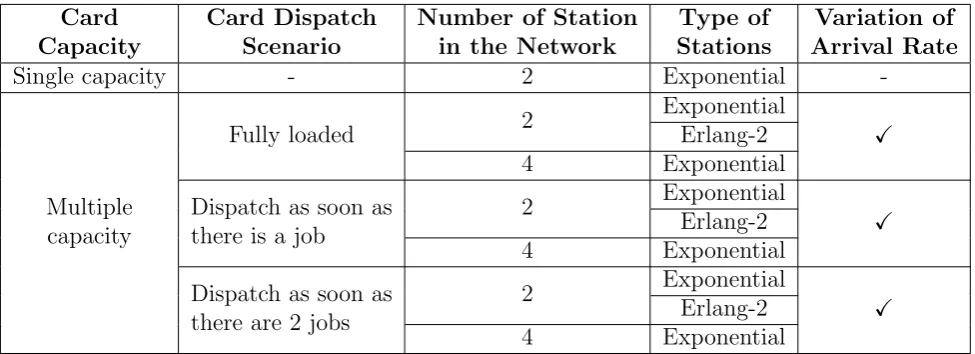
[image:26.595.72.560.305.482.2]

In this report, the performance measure of interest is the mean throughput time of a job, E[T T]. We validate the approximation model using simulation. The simulation is developed using the Python programming language. We run the simulation for a five years simulation period with six months of warm-up period. The purpose of the simulation is to obtain the steady state behavior of the system. Interarrival and service times in the system are in minutes. The proposed approximation model is validated for variety of cases as shown in Table 1. The number of replications for each case is 25.

Table 1: Numerical Experiments

Card Capacity

Card Dispatch Scenario

Number of Station in the Network

Type of Stations

Variation of Arrival Rate

Single capacity - 2 Exponential

-Multiple capacity

Fully loaded 2

Exponential

X

Erlang-2 4 Exponential Dispatch as soon as

there is a job

2 Exponential

X

Erlang-2 4 Exponential Dispatch as soon as

there are 2 jobs

2 Exponential

X

Erlang-2 4 Exponential

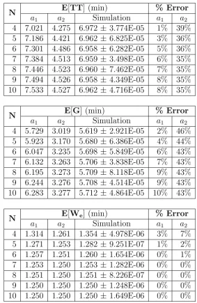
The results are summarized in Table 10 - 14 where E[G] denotes the mean service time of a batch, E[We] denotes the mean waiting time of a job at the external queue, and N

denotes the number of cards. The percentage of error is calculated as follows:

% error = |Approximation - Simulation|

Simulation x 100%.

[image:26.595.74.556.306.482.2]

Column a1 denotes the approximation of the mean and variance of service time G using equation (37) and equation (38), respectively. Columna2 denotes the approximation of the mean and variance of service time E[G] using equation (39) and equation (40), respectively. Column Literature denotes the results of the existing approximation.

Table 3 - 5 show the results for a fully loaded dispatch scenario with card capacity

(27)

the approximation a1 is small compared to the approximation a2. It is also shown that the mean throughput time of a job is increasing as the number of cards increases. This contradict with common case, that the throughput time of a job decreases as the number of cards increases. The reason of the contradiction is because the increment of the mean service time (E[G]), is higher than the decrement of the mean waiting time at the external queue which yields an increasing value of mean throughput time.

Besides comparison with simulation, we also compare the proposed approximation with the existing approximation provided in [3] for the case of single capacity card. It can be seen from Table 10 that our approximation model underestimate the mean throughput time of the system with the highest percentage of 16% for approximation a1 and up to 52% for approximation a2. Meanwhile, the existing approximation overestimate the mean throughput time of the system with maximum error of 5%. We also conduct a numerical experiments for larger network as shown in Table 8 and 9.

The results for the case of a non fully loaded scenario are summarized in Table 11 -14. In this case, we only consider approximation a1 since even for a fully loaded case, the approximation a2 already gives a high percentage of error. There is a large error in the mean waiting time at the external queue of the proposed approximation model a1. This is because when arrival rate of a job is low, the waiting probability is much lower that the the mean waiting time and this yields a large value of the first term of equation (46) and eventually overestimate the mean waiting time during busy period. Specifically, the main error is due to the assumption of the independence of stations in the networks which leads to an underestimation of the variance of service time, Var(G).

In the following table, we present the mean throughput time of a job with two different dispatch scenario. D1 and D2 denote the case of dispatch scenario with d = 1, d = 2, respectively and card capacity ofc= 5. The service time is computed using approximation

(28)

[image:28.595.211.392.136.272.2]

Table 2: Throughput time of a job with different dispatch scenario

N λ =0.2 λ =0.3

D1 D2 D1 D2

4 5.893 6.995 7.075 7.023 5 5.912 7.042 7.325 7.063 6 5.965 7.084 7.551 7.104 7 6.027 7.120 7.754 7.142 8 6.087 7.150 7.936 7.180 9 6.140 7.176 8.097 7.223 10 6.186 7.201 8.240 7.284

5 Conclusion and Recommendations

5.1 Conclusion

In drawing the conclusion for this research, we consider the research question:

What is the best card dispatch scenario such that performance of the system is optimal?

We develop an approximation model based on a decomposition technique. From the re-sults, it can be concluded that for a low arrival rate, dispatching a card only if there are two jobs increases the mean throughput time. Meanwhile, for a relatively high arrival rate, dis-patching the card only if there are two jobs decreases the mean throughput time compared to dispatching the card as soon as there is job at the external queue. However, it is worth to note that having a good approximation model plays important role. In comparison with simulation, the proposed approximation model generally is a poor approximation.

5.2 Recommendations

Future research can be done to obtain a better approximation of PAC systems. The idea of improvements are the following.

1. Relaxation of the assumption of an exponential arrival rate of cards in analyzing synchronization station.

(29)

3. Analyzing the system by decomposition of its busy and free period. During a free period, a PAC system can be modeled as a state-dependent queuing system while during a busy period, the PAC system can be modeled as a multi-server queuing system during its busy period.

(30)

References

[1] Buzacott, J.A., Shanthikumar, J.G., 1993, Stochastic Models of Manufacturing Sys-tems, Prentice Hall. ISBN 0-13-847567-9.

[2] Baldwin, R.O, Davis, N.J., Midkiff, S.F., Kozva, J.E., 2003,Queuing network analysis: concepts, terminology and methods. The Journal of System and Software 66:99-117.

[3] Buithenhek, R., 1998,Performance Evaluation of Dual Resource Manufacturing Sys-tems. PhD thesis, University of Twente.

[4] Briksorn, D., Drexl, A., Hartmann, S., 2006,Inventory-based dispatching of automated guided vehicles on container terminal, OR Spectrum 28:611-630.

[5] Ekren, B.A, Heragu, S.S, Krishnamurthy,A., Malmborg, C.J, 2013, Matrix-geometric solution for SOQN model of autonomous vehicle storage and retrieval system, Com-puters & Industrial Engineering 68:78-86.

[6] Jian, J., Heragu,S.S., 2009,Solving semi-open queueing networks, Operation Research 57(2):391-401.

[7] Kimura, T., 1994, Approximation for Multi-server Queues: system interpolations, Queuing System 17:347-382.

[8] Mishra, N. and Roy, D., van Ommeren, J.C.W., 2013, A stochastic model for inter-terminal container transportation, Memorandum 2032, Department of Applied Math-ematics, University of Twente, Enschede. ISSN 1874-4850.

(31)

[10] Roy, D., Krishnamurthy, A., Heragu, S.S, Malmborg, C.J, 2015, Queuing models to analyze dwell-point and cross aisle location in autonomous vehicle-based warehouse systems, European Journal of Operational Research 242:72-87.

[11] Roy, D., Bandyopadhyay, A., Banerjee, P., 2016, A nested semi-open queuing net-work model for analyzing dine-in restaurant performance, Computers & Operations Research 65:29-41.

[12] Sadowsky, J.S., Szpankowski, W.,1989,On the Analysis of the Tail Queue Length and Waiting Time Distribution of a GI/GI/c queue, Computer Science Technical Reports. Retrieved from http://docs.lib.purdue.edu/cstech/797.

[13] Tierney, K., Voss, S., Stahlbock, R., 2014, A mathematical model of inter-terminal transportation, European Journal of Operational Research 235:448-460.

[14] Xiaobo, Z., Zhou, Z., 1999, A semi-open decomposition approach for an open queuing network in a general configuration with kanban blocking mechanism, Int. J. Production Economics 60-61:375-380.

(32)

(33)

[image:33.595.161.446.264.707.2]

In this appendix, we provide tables that show the results of the numerical experiments for various cases as mention in section 4. Column a1 denotes the approximation of the mean and variance of service time G using equation (37) and equation (38), respectively. Column a2 denotes the approximation of the mean and variance of service time E[G] using equation (39) and equation (40), respectively. Table 3 - 5 show the results for a fully loaded dispatch scenario for different types of network.

Table 3: Card capacity c= 2 with two-stations exponential network, λ= 0.3 jobs per min, µ1 =µ2 = 0.5 batch per min

.

N E[TT] (min) % Error

a1 a2 Simulation a1 a2 4 6.933 3.972 6.656 ± 2.378E-05 4% 40% 5 7.016 4.010 6.651 ± 4.467E-05 5% 40% 6 7.072 4.021 6.648 ± 3.934E-05 6% 40% 7 7.112 4.024 6.653 ± 4.615E-05 7% 40% 8 7.143 4.024 6.652 ± 3.615E-05 7% 40% 9 7.167 4.023 6.654 ± 2.442E-05 8% 40% 10 7.187 4.022 6.650 ± 2.763E-05 8% 40%

N E[G] (min) % Error

N E[We] (min) % Error

(34)

[image:34.595.162.446.222.658.2]

Table 4: Card capacity c= 2 with two-stations exponential network, λ= 0.4 jobs per min, µ1 =µ2 = 0.5 jobs per min

.

(35)

[image:35.595.162.447.220.660.2]

Table 5: Card capacity c= 2 with two-stations exponential network, λ= 0.5 jobs per min, µ1 =µ2 = 0.5 jobs per min

.

(36)

[image:36.595.158.450.222.658.2]

Table 6: Card capacity c= 2 with two-stations Erlang-2 network, λ= 0.7 jobs per min,

µ1 = 2 jobs per min, µ2 = 1 jobs per min

.

a1 a2 Simulation a1 a2 4 5.650 3.265 6.034 ± 7.267E-05 6% 46% 5 6.052 3.703 6.031 ± 5.086E-05 0% 39% 6 6.391 4.022 6.0301± 7.376E-05 6% 33% 7 6.671 4.249 6.032 ± 4.842E-05 11% 30% 8 6.898 4.411 6.033 ± 6.184E-05 14% 27% 9 7.081 4.524 6.033 ±1.119E-04 17% 25% 10 7.230 4.604 6.029 ± 9.746E-05 20% 24%

(37)

[image:37.595.161.448.219.660.2]

Table 7: Card capacity c= 2 with two-stations Erlang-2 network, λ= 0.8 jobs per min,

µ1 = 2 jobs per min µ2 = 1 jobs per min

.

(38)

[image:38.595.160.448.218.660.2]

Table 8: Card capacity c= 2 with four-stations exponential network, λ= 0.2 jobs per min, µ1 =µ2 = 0.5, µ3 = 1.0, µ4 = 1.5 batch per min

.

a1 a2 Simulation a1 a2 4 6.529 2.788 6.239 ± 2.037E-05 5 % 55 % 5 6.583 2.784 6.244 ± 4.515E-05 5 % 55 % 6 6.620 2.782 6.243 ± 3.397E-05 6 % 55 % 7 6.647 2.781 6.242 ± 2.634E-05 6 % 55 % 8 6.667 2.780 6.244 ± 3.036E-05 7 % 55 % 9 6.683 2.779 6.242 ± 2.586E-05 7 % 55 % 10 6.697 2.779 6.239 ± 5.175E-05 7 % 55 %

(39)

[image:39.595.164.451.223.659.2]

Table 9: Card capacity c = 2 with four-stations exponential network, λ = 0.3, µ1 =µ2 = 0.5, µ3 = 1.0, µ4 = 1.5

.

a1 a2 Simulation a1 a2 4 6.982 4.036 6.807 ± 3.482E-05 3 % 41 % 5 7.107 4.018 6.826 ± 6.168E-05 4 % 41 % 6 7.189 4.009 6.837 ± 7.245E-05 5 % 41 % 7 7.246 4.005 6.835 ± 2.992E-05 6 % 41 % 8 7.291 4.002 6.834 ± 4.012E-05 7 % 41 % 9 7.325 4.000 6.829 ± 4.398E-05 7 % 41 % 10 7.354 3.998 6.834 ± 2.249E-05 8 % 41 %

(40)

[image:40.595.101.509.232.674.2]

This table shows the comparison between our approximation model with an existing approximation (Column Literature).

Table 10: Single capacity with two-stations exponential network, λ = 0.2 jobs per min,

µ1 =µ2 = 0.5 jobs per min.

Literature a1 a2 Simulation Literature a1 a2 4 7.115 5.651 3.284 6.732 ± 2.18E-04 6 % 16 % 51 % 5 6.853 5.789 3.255 6.691 ± 2.62E-04 2 % 13 % 51 % 6 6.745 5.906 3.240 6.673 ± 2.51E-04 1 % 12 % 51 % 7 6.699 6.000 3.233 6.663 ± 3.02E-04 0 % 10 % 52 % 8 6.681 6.074 3.228 6.663 ± 2.19E-04 0 % 9 % 52 % 9 6.673 6.134 3.225 6.663 ± 1.38E-04 0 % 8 % 52 % 10 6.669 6.184 3.222 6.663 ± 1.51E-04 1 % 7 % 51 %

Literature a1 a2 Simulation Literature a1 a2 4 6.634 5.582 3.270 6.337 ± 2.886E-05 5 % 12 % 48 % 5 6.652 5.767 3.250 6.507 ± 3.913E-05 5 % 9 % 49 % 6 6.659 5.898 3.239 6.595 ± 6.843E-05 5 % 7 % 49 % 7 6.663 5.997 3.233 6.639 ± 5.639E-05 5 % 5 % 49 % 8 6.665 6.073 3.228 6.657 ± 1.943E-04 5 % 4 % 49 % 9 6.666 6.134 3.225 6.654 ± 9.100E-05 5 % 3 % 49 % 10 6.666 6.183 3.222 6.664 ± 1.053E-04 5 % 2 % 49 %

(41)

[image:41.595.186.423.236.666.2]

The following tables show the result for a non fully loaded dispatch scenario for a two stations network.

Table 11: Mininum card capacity d = 1, maximum card capacity c = 5, λ = 0.2, µ1 = µ2 = 0.5

.

a1 Simulation

4 5.893 6.604 ± 6.969E-05 11% 5 5.912 6.628 ± 8.861E-05 11% 6 5.965 6.640 ±1.209E-04 10% 7 6.027 6.656 ± 2.463E-04 9% 8 6.087 6.664 ± 7.422E-05 9% 9 6.140 6.665 ± 8.618E-05 8% 10 6.186 6.668 ± 5.618E-05 7%

a1 Simulation

4 5.582 6.295 ± 2.966E-05 11% 5 5.767 6.487 ± 4.777E-05 11% 6 5.898 6.578 ± 7.921E-05 10% 7 5.997 6.629 ± 1.593E-04 10% 8 6.073 6.651 ± 6.969E-05 9% 9 6.134 6.660 ± 8.410E-05 8% 10 6.183 6.666 ± 5.579E-05 7%

a1 Simulation

(42)

[image:42.595.185.420.224.648.2]

a1 Simulation

4 7.075 8.801 ± 6.969E-05 20% 5 7.325 9.066 ± 8.861E-05 19% 6 7.551 9.287 ± 1.208E-04 19% 7 7.754 9.481 ± 2.463E-04 18% 8 7.936 9.608 ± 2.317E-04 17% 9 8.097 9.721 ± 2.139E-04 17% 10 8.240 9.804 ± 1.473E-04 16%

a1 Simulation

4 6.426 7.636 ± 2.966E-05 16% 5 6.899 8.304 ± 4.777E-05 17% 6 7.270 8.788 ± 7.921E-05 17% 7 7.569 9.153 ± 1.593E-04 17% 8 7.814 9.397 ± 1.699E-04 17% 9 8.017 9.584 ± 1.704E-04 16% 10 8.188 9.715 ± 1.305E-04 16%

a1 Simulation

(43)

[image:43.595.186.423.221.652.2]

.

a1 Simulation

4 7.313 6.980 ± 2.255E-05 5% 5 7.334 6.980 ± 4.042E-05 5% 6 7.356 6.978 ± 2.407E-05 5% 7 7.374 6.977 ± 3.309E-05 6% 8 7.390 6.977 ± 2.279E-05 6% 9 7.403 6.977 ± 3.309E-05 6% 10 7.415 6.978 ± 4.477E-05 6%

a1 Simulation

4 4.784 4.478 ± 1.212E-05 7% 5 4.825 4.481 ± 3.118E-05 8% 6 4.852 4.475 ± 2.407E-05 8% 7 4.871 4.478 ± 3.309E-05 9% 8 4.886 4.476 ± 2.278E-05 9% 9 4.898 4.478 ± 3.309E-05 9% 10 4.908 4.478 ± 4.477E-05 10%

a1 Simulation

(44)

[image:44.595.186.424.224.653.2]

.

a1 Simulation

4 6.995 6.647 ± 3.346E-05 5% 5 7.042 6.649 ± 3.198E-05 6% 6 7.084 6.650 ± 4.603E-05 7% 7 7.120 6.649 ± 2.968E-05 7% 8 7.150 6.652 ± 5.579E-05 7% 9 7.176 6.652 ± 4.298E-05 8% 10 7.201 6.649 ± 3.034E-05 8%

a1 Simulation

4 5.251 4.964 ± 3.410E-05 6% 5 5.346 4.980 ± 3.400E-05 7% 6 5.404 4.983 ± 4.056E-05 8% 7 5.445 4.984 ± 4.579E-05 9% 8 5.476 4.986 ± 4.783E-05 10% 9 5.500 4.986 ± 2.769E-05 10% 10 5.520 4.982 ± 3.193E-05 11%

a1 Simulation