University of Warwick institutional repository: http://go.warwick.ac.uk/wrap
This paper is made available online in accordance with
publisher policies. Please scroll down to view the document
itself. Please refer to the repository record for this item and our
policy information available from the repository home page for
further information.
To see the final version of this paper please visit the publisher’s website.
Access to the published version may require a subscription.
Author(s): Lucio Sarno, Daniel L. Thornton and Giorgio Valente
Article Title: The Empirical Failure of the Expectations Hypothesis of the
Term Structure of Bond Yields
Year of publication: 2007
Link to published version: http://dx.doi.org/
10.1017/S0022109000002192
The Empirical Failure of the Expectations
Hypothesis of the Term Structure of Bond
Yields
Lucio Sarno, Daniel L. Thornton, and Giorgio Valente
∗Abstract
This paper tests the expectations hypothesis (EH) using U.S. monthly data for bond yields spanning the 1952–2003 sample period and ranging in maturity from one month to 10 years. We apply the Lagrange multiplier test developed by Bekaert and Hodrick (2001) and extend it to increase the test power by introducing economic variables as conditioning information and by using more than two bond yields in the model and testing the EH jointly on more than one pair of yields. While the conventional bivariate procedure provides mixed results, the more powerful testing procedures suggest rejection of the EH throughout the maturity spectrum examined.
I.
Introduction
The expectations hypothesis (EH) of the term structure of interest rates is the proposition that the long-term rate is determined by the market’s expectation for the short-term rate plus a constant risk premium. The EH plays an important role in economics andfinance, so it is not surprising that it has been investigated thoroughly using a variety of tests and data (e.g., Campbell and Shiller (1991), Frankel and Froot (1987), Froot (1989), and Bekaert and Hodrick (2001)). It is well known that the tests that are commonly used to investigate the EH tend to generate paradoxical results (Campbell and Shiller (1991)). Recently, Bekaert, Hodrick, and Marshall (1997) show that one of these tests can yield results that
∗Sarno, lucio.sarno@warwick.ac.uk, Finance Group, Warwick Business School, University of
Warwick, Coventry, CV4 7AL, UK, Thornton, thornton@stls.frb.org, Federal Reserve Bank of St. Louis, PO Box 442, St. Louis, MO 63166, and Valente, giorgio.valente@cuhk.edu.hk, Department of Finance, The Chinese University of Hong Kong, Shatin, N.T., Hong Kong. The authors are indebted to Geert Bekaert (the referee), Stephen Brown (the editor), John Campbell, Rob Dittmar, Robert Ho-drick, and Jennifer Roush for their constructive comments on earlier drafts of this paper. They are also grateful to Bob Bliss and Dan Waggoner for providing the FORTRAN codes designed to calculate the bond yields used in this paper and for useful conversations. Pasquale Della Corte, Stephen Gardner, and John Zhu provided excellent research assistance. The views expressed here are the authors’ alone and do not necessarily reflect the views of the Board of Governors of the Federal Reserve System or the Federal Reserve Bank of St. Louis.
are unduly favorable to the EH when it is true, while Thornton (2006) shows that this test can yield results that are favorable to the EH when it is false.1
Given the statistical problems afflicting conventional tests of the EH, in this paper we employ a test that was originally proposed by Campbell and Shiller (1987) and recently made operational by Bekaert and Hodrick (2001) who de-velop a procedure for testing the parameter restrictions that the EH imposes on a vector autoregression (VAR) of the short- and long-term interest rates using a Lagrange multiplier (LM) test. The procedure isflexible and its size and power properties have been thoroughly investigated by Bekaert and Hodrick (2001). We apply this test to a data set for U.S. bond yields ranging in maturity from one month to 10 years over the sample period 1952–2003.2
In order to increase the power of the EH testing procedure, we move beyond the bivariate comparisons of short- and long-term yields that dominate the exist-ing literature. First, inspired by the growexist-ing literature linkexist-ing macroeconomic fundamentals to the behavior of the term structure of interest rates (e.g., Kozicki and Tinsley (2001), Evans and Marshall (2002), Ang and Piazzesi (2003), Ang, Piazzesi, and Wei (2003), Bekaert, Cho, and Moreno (2004), Rudebusch and Wu (2004), Carriero, Favero, and Kaminska (2006), Dewachter and Lyrio (2006), Diebold, Rudebusch, and Aruoba (2006), and Clarida, Sarno, Taylor, and Valente (2006)), we investigate the possibility of increasing the power of the EH testing procedure by examining the linkage between the term structure and macroeco-nomic variables used as conditioning information. Second, we attempt to increase test power by using more than two yields in the VAR model and testing the EH on more than one pair of rates.
To anticipate our results, wefind that the conventional bivariate procedure provides mixed results, suggesting that the EH is rejected at the short end of the maturity spectrum but not at the longer end. Specifically, consistent with a vast body of previous results (e.g., Campbell and Shiller (1991)), the EH is nearly always rejected when the maturity of the long-term rate is 24 months or shorter, but it is usually not rejected when the long-term rate is longer than 24 months. The more powerful procedures based on expanded VARs either with macroeconomic factors or with more than two bond yields suggest a more widespread rejection of the EH. In particular, the test based on a VAR including more than two bond yields suggests rejection of the EH throughout the maturity spectrum from one month to 10 years. Finally, the increase in power is documented using a simple Monte Carlo exercise designed to quantify the power gain obtained by moving from the bivariate VAR for bond yields to VARs that involve economic variables or more than two bond yields.
The outline of the paper is as follows. Section II presents the essential ingre-dients of the LM test proposed by Bekaert and Hodrick (2001). Section III briefly describes the data and preliminary unit root tests on our bond yields designed to
1Moreover, Kool and Thornton (2004) and Thornton (2005) show how conventional tests may
have generated misleading results in applied work.
2In a previous draft of this paper, we used the data set used by Campbell and Shiller (1991) in their
verify the validity of the stationarity condition required by the LM testing proce-dure. In Section IV, the LM test is applied to our data in three different settings: i) the conventional bivariate VAR designed to make all possible pairwise com-parisons among our 12 bond yields; ii) the expanded VAR that includes other economic variables as conditioning information; and iii) the expanded VAR that includes more than two bond yields. We report some Monte Carlo results to mea-sure the empirical power of our testing procedures and some robustness checks in Section V. The conclusions are presented in Section VI.
II.
The VAR Test of the EH
The EH asserts that the long-term rate is determined by the market’s expec-tation for the short-term rate over the holding period of the long-term asset plus a constant risk premium,
rn
t = (1/k)
k−1
i=0 Etr
m
t+mi+πn,m,
(1)
wherern
t is then-period (long-term) rate, rtm is them-period (short-term) rate, πn,mis the constant risk premium that may vary with the maturity of the rates, Etis the expectations operator, andk=n/mis an integer.3 Much of the relevant
literature relies on tests of the EH that are derived by parameterizing an algebraic manipulation of equation (1). In contrast, Bekaert and Hodrick’s (2001) procedure assumes that the long- and short-term rates can be represented by a general VAR specification and test the restrictions implied by the EH on the VAR. Because a general VAR encompasses a wider range of potential data generating processes (DGPs) than equation (1), it is reasonable to conjecture that tests based on the VAR specification will be more powerful than tests derived from equation (1). In addition, the VAR approach has the advantage of being easy to extend—albeit computationally more intensive—by including more than two interest rates or incorporating conditioning variables that might affect market expectations.
The VAR restrictions implied by the EH are highly nonlinear, and Bekaert and Hodrick (2001) propose and study the properties of various tests for these restrictions. Their Monte Carlo evidence suggests that, while the distance metric, Wald, and LM tests all exhibit size distortions, the LM test displays considerably better size properties. For a 5% nominal test, the empirical size of the LM test varied between 0.7% and 7.9%. In half of the cases, the empirical size was within one percentage point of the nominal size. Moreover, the LM test had reasonable power. Tofit a VAR to interest rates data that satisfy the restrictions imposed by the EH, we use the constrained Generalized Method of Moments (GMM) esti-mation described in Bekaert and Hodrick (2001). As this procedure is relatively new, it is briefly presented here. Considering the EH for two bond yields, the VAR takes the form,
(I−Θ(L))yt+1 = ηt+1, (2)
3Shiller, Campbell, and Schoenholtz (1983) show that equation (1) is exact in some special cases
foryt ≡ (rm
t ,rtn),Iis the 2×2 identity matrix,Θ(L)is a lag polynomial, and ηt+1 is a vector of error terms. Letg(zt, θ) ≡ ηt⊗xt−1, wherext−1 is a vector formed from stacking lagged values ofyt, and possibly with a constant term. zt
is defined as(y
t,xt−1), andθis a vector formed from the parameters inΘ(L). GMM estimation imposes orthogonality conditions of the formE[g(zt, θ)] =0. Using the sample moment condition,
gT(θ) ≡ T1
T
t=1
g(zt, θ),
(3)
GMM estimation proceeds by choosingθto minimize the following GMM crite-rion function,
JT(θ) ≡ gT(θ)WgT(θ).
(4)
The optimal weighting matrix, W, is defined as the inverse of Ω ≡ kk==∞−∞ E[g(zt, θ)g(zt−k, θ)](Hansen (1982)). We can use GMM to estimate restricted
VARs by forming a Lagrangian from the usual GMM quadratic objective function and a vector of parameter constraints. The Lagrangian is defined as
L(θ, γ) = −12gT(θ)Ω−1
T gT(θ)−aT(θ)γ,
(5)
whereγis a vector of LMs and the constraints onθhave been represented by the vector valued function,aT(θ) =0. Here the matrixΩTis a consistent estimate of
the matrixΩdefined above.
In constructing our constrained estimates, we begin with the unconstrained VAR parameters and iterate until the constraints are satisfied. The constraints that the EH imposes on a VAR can be seen by writing the VAR infirst-order form, that is ⎛ ⎜ ⎜ ⎜ ⎜ ⎜ ⎜ ⎜ ⎜ ⎜ ⎝ rm t rn t rm t−1
rn t−1
.. . rm t−k rn t−k ⎞ ⎟ ⎟ ⎟ ⎟ ⎟ ⎟ ⎟ ⎟ ⎟ ⎠ = ⎛ ⎜ ⎜ ⎜ ⎜ ⎜ ⎜ ⎝
θ1 θ2 · · · θr
I 0 0
0 I ...
..
. ...
0 I 0
⎞ ⎟ ⎟ ⎟ ⎟ ⎟ ⎟ ⎠ ⎛ ⎜ ⎜ ⎜ ⎜ ⎜ ⎜ ⎜ ⎜ ⎜ ⎝ rm t−1
rn t−1
rm t−2
rn t−2
.. .
rm t−k−1
rn t−k−1
⎞ ⎟ ⎟ ⎟ ⎟ ⎟ ⎟ ⎟ ⎟ ⎟ ⎠ + ⎛ ⎜ ⎜ ⎜ ⎝ ηt 0 .. . 0 ⎞ ⎟ ⎟ ⎟ ⎠, (6)
or simplyxt+1=Γxt+υt+1. Note thatEt(xt+k) =Γkxt, so thatEt(rmt+k) =e1Γkxtfor
e1=(1,0, . . . ,0). Note, too, thatrtn=e2xtfore2=(0,1,0, . . . ,0). Consequently, for any two bond yields such thatk=n/mis an integer, the EH implies that
rnt =
1
k k−1
i=0
Et(rtm+mi),
(7)
so that the EH can be equivalently expressed as
e2xt = 1k
k−1
i=0
e1Γmixt.
The constraints that satisfy the EH are given by
aT(θ) ≡ e
2− 1
k k−1
i=0
e
1Γmi = 0.
(9)
No simple closed form exists for the Jacobian of these constraints. Consequently, they are calculated numerically. The iterative method used in this paper is the Broyden-Fletcher-Goldfarb-Shanno (BFGS) method for numerical optimization. If the constraints have a significant impact on parameter estimation, then the es-timated LMs should be significantly different from zero. Bekaert and Hodrick (2001) derive the asymptotic distribution of the LM test statistic for the null hy-pothesis that the multipliers are jointly zero, i.e., for the hyhy-pothesis that the EH of the term structure of interest rates is valid. The LM test statistic is asymptotically distributed asχ2(l), wherelis the number of constraints.4
III.
Data and Preliminary Unit Root Tests
We use continuously compounded yields on riskless pure discount bonds for the U.S. These yields are calculated using end-of-month observations for bonds ranging in maturity from 1 to 120 months (or 10 years) over the period 1952:01 to 2003:12, taken from Bloomberg. The continuously compounded yields on risk-less pure discount bonds are obtained using FORTRAN codes kindly provided by Robert Bliss and Dan Waggoner, based on Bliss (1997) and Waggoner (1997). The estimation method is based on the McCulloch cubic spline parameters, esti-mated using programs originally provided by J. Huston McCulloch.
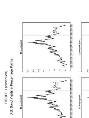
In order to check the quality of our resulting data set, we compare our time series for continuously compounded yields on riskless pure discount bonds to the equivalent time series obtained by McCulloch and Kwon (1993) in construct-ing an update of the data used by Campbell and Shiller (1991). Figure 1 graphs our time series of bond yields over the full sample period 1952:1–2003:12 (dot-ted line) and the corresponding bond yields calcula(dot-ted by McCulloch and Kwon (1993) over the shorter sample period 1952:1–1991:02 (solid bold line). The graphs confirm that the time series are virtually identical for the overlapping pe-riod, so that our series may be considered as a consistent update of the data used by Campbell and Shiller (1991) and McCulloch and Kwon (1993).
As an important preliminary to the implementation of the procedure for test-ing the EH, we tested for unit root behavior of each of the bond yields examined.5 This exercise is relevant since the VAR test described in Section II and its ex-panded version considered in the empirical work rely on the assumption that bond yields are stationary. Whilefinance theory is generally based on the assumption 4See Bekaert and Hodrick (2001) for a full technical exposition of the iterative procedure and
the asymptotic distribution of the LM statistic. Note that the above analysis presumes that the short-and long-term rates are stationary, orI(0). If rates areI(1), the above procedure needs amending, which may be done by building on the work of Campbell and Shiller (1987). See also Hall, Anderson, and Granger (1992), Engsted and Tanggaard (1994), Sarno and Thornton (2003), and Clarida, Sarno, Taylor, and Valente (2006).
5In all statistical tests executed in this and subsequent sections, we use a 5% nominal significance
that interest rates are stationary, and we have a strong economic prior that this is the case, it is often difficult to provide empirical evidence against the hypothesis that interest rates have a unit root. This is likely to be due to the low power of most conventional unit root tests in the presence offinite sample realizations of persistent—albeit stationary—processes with a root strictly below but very close to unity (e.g., Stock and Watson (1988), (1999)).
We rely on two different unit root tests: the test proposed by Kwiatkowski, Phillips, Schmidt, and Shin (1992), the KPSS test, for the null hypothesis of sta-tionarity; and the point optimal unit root test proposed by Elliott, Rothenberg, and Stock (1996), thePT test, for the null hypothesis of a unit root. The latter test is
the unit root test that was found to exhibit the best power properties among the several tests investigated by Elliott, Rothenberg, and Stock (1996).
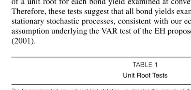
[image:9.612.63.383.356.508.2]The results from applying both test statistics are reported in Table 1. For each time series considered, we selected the lag length on the basis of the Akaike information criterion. The results indicate that the KPSS test fails to reject the null of stationarity in each case, whereas thePTtest statistic rejects the null hypothesis of a unit root for each bond yield examined at conventional significance levels. Therefore, these tests suggest that all bond yields examined are realizations from stationary stochastic processes, consistent with our economic prior and with the assumption underlying the VAR test of the EH proposed by Bekaert and Hodrick (2001).
TABLE 1
Unit Root Tests
The figures reported are unit root test statistics. mdenotes the maturity of the zero-coupon bond. PT is the Elliott,
Rothenberg, and Stock (1996) point optimal unit root test of the null hypothesis that the time series contains a unit root. KPSS is the Kwiatkowski, Phillips, Schmidt, and Shin (1992) test of the null hypothesis that the series is stationary. Both test statistics have been computed by estimating the residual spectrum at frequency zero by means of the Andrews’ (1991) rule with a quadratic spectral kernel. The 5% critical values are 3.26 (Elliott, Rothenberg, and Stock (1996), Table 1) and 0.463 (Kwiatkowski, Phillips, Schmidt, and Shin (1992), Table 1) for thePTand KPSS test, respectively.
m PT KPSS
1 4.590 0.174
2 5.112 0.157
3 5.383 0.154
4 5.560 0.152
6 5.593 0.150
9 5.823 0.149
12 6.404 0.151
24 8.246 0.161
36 9.837 0.172
48 11.380 0.182
60 12.875 0.193
120 18.390 0.246
IV.
The VAR Test Results
The data were adjusted for their mean prior to carrying out the VAR tests. The order of the VAR is determined by minimizing the Akaike information crite-rion.
A. VAR Tests for Bivariate Comparisons of Bond Yields
Bekaert, Hodrick, and Marshall (1997) show significant bias in standard tests of the EH because of the extreme persistence in short-term rates. Bekaert and Ho-drick (2001) show that this bias is reduced, but not eliminated in the VAR test they propose. Following Bekaert and Hodrick (2001), we correct for this bias by using the unconstrained estimates of the VAR for each rate pair to generate 100,000 artificial data sets of the sample size corresponding to each pair of rates using i.i.d. bootstraps of the residuals. The VAR parameters are reestimated to determine the bias—the difference between the average value of these parameters and the known values of the data generating process. These estimates are used to correct for the bias of the original VAR estimates. Bias-corrected parameters that satisfy the EH are obtained by using the unconstrained, bias-corrected parameters and residuals to simulate a series of 71,000 observations, with the initial 1,000 observations discarded. The bias-corrected, constrained parameters are obtained from implementing the procedure described in Section II. The empirical distribu-tion for the bias-corrected LM statistics is then obtained from 25,000 replicadistribu-tions of this procedure applied to artificial data obtained using the bias-corrected, con-strained parameters and the corresponding residuals. The empirical distribution and critical values for the LM statistics are relatively unaffected by the choice of maturity pair. Nevertheless, the asymptotic critical values are always smaller than the bootstrapped critical values. Hence, while in many cases, consistent with Bekaert and Hodrick’s (2001)findings, the size distortions of the LM test are rel-atively small, this was not uniformly the case. These results suggest that using the asymptotic critical values can be misleading and, therefore, we rely on the empirical distribution in our analysis.
The LM test results are presented in Table 2, where we report thep-values for the null hypothesis that the EH holds for all possible combinations of the integer
k=n/m(there are 48 such combinations). Thefigures in bold denote cases where the null hypothesis is not rejected at the 5% significance level. Consistent with Campbell and Shiller (1991), the EH is always rejected at the shorter end of the maturity spectrum, but not at the longer end. Specifically, the EH is rejected in every case where the long-term rate is two years or shorter or, put another way, the EH is not rejected only in instances where the long-term rate is three years or longer.
Another way to evaluate the EH is by assessing its forecasting accuracy: if the EH is valid, one should be able to forecast the long-term rate by making the forecasts conditional on the information embedded in the EH. To this end, Campbell and Shiller (1987), (1991) suggest comparing the ratio of the variance of the “theoretical” long-term rate to the variance of the actual data, where the theoretical long-term rate is the rate under the assumption that the EH holds.6 In
6The theoretical rate isrn
t = (1/k)e1(I−Γn)(I−Γm)−1yt, wheree1andΓare as defined in
TABLE 2
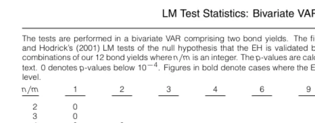
LM Test Statistics: Bivariate VAR
The tests are performed in a bivariate VAR comprising two bond yields. The figures reported arep-values of Bekaert and Hodrick’s (2001) LM tests of the null hypothesis that the EH is validated by the data for each of the possible 48 combinations of our 12 bond yields wheren/mis an integer. Thep-values are calculated by bootstrap as described in the text. 0 denotesp-values below 10−4. Figures in bold denote cases where the EH is not rejected at the 5% significance level.
n/m 1 2 3 4 6 9 12 24 60
2 0
3 0
4 0 0
6 0 0 0
9 0 0
12 0 0 0 0 0
24 0.025 0.047 0.018 0.008 0.001 0
36 0.104 0.204 0.143 0.124 0.118 0.092 0.053
48 0.264 0.370 0.304 0.294 0.335 0.022 0.064 60 0.433 0.489 0.427 0.429 0.497 0.114
120 0.828 0.795 0.731 0.751 0.836 0.064 0.057 0.162
order to formally test the EH using the ratios of the variances, we obtained the distributions of these ratios under the null that the EH holds. Specifically, we calculate these ratios for each of 25,000 replications of data generated using the bias-corrected, constrained VAR. Three features of these results are noteworthy.7 First, consistent with the results of Campbell and Shiller (1991), these ratios are always less than unity, suggesting that the long-term rate is too variable to be consistent with the EH. Second, the forecast accuracy declines askincreases or as (n−m)increases for a given value ofk. This is reflected by the fact that these ratios decline asn increases for a givenm, suggesting that the forecasting accuracy declines as the forecast horizon lengthens. Third, these ratios tend to be closer to unity when the EH is rejected by the LM test than when it is not. Hence, the size of the ratio appears to be a misleading indicator of the validity of the EH. Consistent with the results of the LM test, the results indicate that the EH is rejected at the short end of the maturity spectrum but not at the longer end. However, our results suggest that these ratios may be misleading in evaluating the validity of the EH and may be less deserving of attention than the other VAR-based tests. Thisfinding confirms the results of Bekaert, Wei, and Xing (2004) who also investigate the term structure at the long and short end (together with uncovered interest rate parity) and document large biases and widefinite sample distributions of these variance ratio statistics.
B. Extension to Allow Macroeconomic Variables as Conditioning Information
Conceptually, the VAR can also include other economic variables. There is a large and rapidly developing literature on various aspects of the relation between macroeconomic variables and the yield curve (e.g., Kozicki and Tinsley (2001), Evans and Marshall (2002), Ang and Piazzesi (2003), Ang, Piazzesi, and Wei (2003), Bekaert, Cho, and Moreno (2004), Rudebusch and Wu (2004), Carriero, Favero, and Kaminska (2006), Dewachter and Lyrio (2006), Diebold, Rudebusch,
and Aruoba (2006), and Clarida, Sarno, Taylor, and Valente (2006)). This interest is in part motivated by the realization that, while the term structure can be well characterized by a few latent factors, such analyses provide little insight into the forces that shift or rotate the term structure. It is also motivated by the realization that macroeconomic forces may drive the principal determinants of nominal in-terest rates (inflation and the real economy), and by the fact that monetary policy actions—which are in large part driven by these same forces—have consequences for short-term rates that are crucial to the rest of the term structure.
For example, Gurkaynak, Sack, and Swanson (2005) show that long-term rates respond significantly to macroeconomic surprises that should have only a transitory effect on short-term interest rates. They interpret this to be evidence that market participants adjust their expectations of long-run inflation in response to such shocks. Clarida, Sarno, Taylor, and Valente (2006) examine the relation between interest rates of different maturities for the U.S., Germany, and Japan over the period 1982–2000 using a multivariate modeling framework capable of simultaneously allowing for asymmetric adjustment and regime shifts that allow for time-varying term premia and other short-run deviations from the EH of the term structure. They show how the term structure of interest rates displays regime switches closely related to key state variables driving monetary policy decisions. This evidence adds to previousfindings that the behavior of the entire yield curve is associated with the state of the business cycle, which may have statistically and economically importantfirst-order effects on expectations of inflation, monetary policy, and nominal interest rates (e.g., Bansal and Zhou (2002)). In any event, recent research suggests an important relation between macroeconomic variables and the term structure. To our knowledge, only Carriero, Favero, and Kaminska (2006) directly investigate the effects of including such variables on the EH. They do not test the EH per se, however. Rather, they assess the benefits from including the macroeconomic variables for forecasts of the short-term rate.
Following Carriero, Favero, and Kaminska (2006), we use the CPI inflation rate and the unemployment rate which, like interest rates, are not subject to re-vision. Preliminary to testing the EH, we tested whether the economic variables were significant in interest rate equations of the VAR using the block exogeneity test suggested by Hamilton (1994). The results, reported in Table 3, indicate that in nearly all cases the null hypothesis of no effect is rejected at the 5% significance level. Hence, including these variables could affect tests of the EH.
The LM tests for the expanded VAR are presented in Table 4, which reports the bootstrappedp-values calculated using the same procedure described in Sec-tion IV.B. Again, thefigures in bold denote cases where the null hypothesis is not rejected at the 5% significance level. The EH is rejected in every case where the long-term rate is three years or shorter and in most cases when the long-term rate is four years. It is generally not rejected when the maturity of the long-term rate isfive or 10 years.
TABLE 3
Block Exogeneity Tests
The tests are performed in a bivariate VAR comprising two bond yields and allowing for two macroeconomic fundamentals (unemployment rate and inflation rate) in each of the two VAR equations. The figures reported arep-values for the likelihood ratio (LR) test of the null hypothesis that the coefficients in the bond yields equations attached to the macroeconomic fundamentals are jointly equal to zero. The test statistics are calculated by using the small-sample correction proposed by Sims ((1980), p. 17). 0 denotesp-values below 10−4. Figures in bold denote cases where the null hypothesis of no block exogeneity is not rejected at the 5% significance level.
n/m 1 2 3 4 6 9 12 24 60
2 0.111 3 0.070
4 0.038 0.007
6 0.053 0.041 0.077
9 0.020 0.023
12 0.001 0.001 0.001 0 0
24 0 0 0 0 0 0
36 0 0 0 0 0 0 0
48 0 0 0 0 0 0 0
60 0 0 0 0 0 0
120 0 0 0 0 0 0 0.001 0.001
TABLE 4
LM Test Statistics: Bivariate VAR with
Macroeconomic Fundamentals as Conditioning Information
The tests are performed in a bivariate VAR comprising two bond yields and allowing for two macroeconomic fundamentals (unemployment rate and inflation rate) in each of the two VAR equations. The figures reported arep-values of Bekaert and Hodrick’s (2001) LM tests of the null hypothesis that the EH is validated by the data for each of the possible 48 combinations of our 12 bond yields wheren/mis an integer. Thep-values are calculated by bootstrap as described in the text. 0 denotesp-values below 10−4. Figures in bold denote cases where the EH is not rejected at the 5% significance level.
n/m 1 2 3 4 6 9 12 24 60
2 0
3 0
4 0 0
6 0 0 0
9 0 0
12 0 0 0 0 0
24 0.001 0 0 0 0 0
36 0.014 0.006 0.017 0.033 0.024 0.011 0.015
48 0.041 0.017 0.032 0.011 0.114 0.125 0.003
60 0.088 0.043 0.117 0.227 0.257 0.308
120 0.304 0.180 0.378 0.571 0.639 0.762 0.519 0.583
of interest rates reflects information contained in these macroeconomic variables and that the test power may be increased by conditioning on macroeconomic in-formation. When this information is accounted for, the marginal information in the long-term rate has relatively little additional information useful for predicting the short-term rate.
C. Extension to Three Bond Yields
the restrictions that satisfy the EH, it can be shown that the results are invariant to how the EH is imposed on then-period rate.8
We applied the Bekaert-Hodrick test to all of the 91 possible three interest rate combinations. Thep-values of the LM tests that the EH holds are reported in Table 5. Unfortunately, the procedure failed to converge in 15 of the 91 cases— denoted as NC in Table 5. In all of these cases where the procedure converged, the EH was overwhelmingly rejected at very low significance levels. Interpreting non-convergence as a rejection of the EH, the evidence is overwhelmingly against the EH when three rates are considered.9The non-convergence does not appear to be related to the model stability. Indeed, the largest root of the unrestricted VAR tends to be smaller for the three interest rates VARs. The evidence suggests that when more than two bond yields are considered, it is less likely that the estimated parameters of the unrestricted VAR will satisfy the restrictions implied by the EH. Note that the increase in power in this case is coming from the fact that the null hypothesis is now a joint hypothesis that the EH holds for two pairs of bond yields. Hence, this is a more stringent test of the EH than the tests based on the bivariate VAR with two bond yields and the VAR with macroeconomic factors, which test the validity of the EH on one pair of bond yields at the time.10
D. Summing Up the Empirical Results from the VAR Tests
Overall, the VAR tests of the EH carried out in this section provide three clear
findings. First, incorporating macroeconomic factors as conditioning information in the VARs enhances the power of the tests for the hypothesis that the EH holds. This is consistent with the exploding literature linking macroeconomic factors to the term structure of interest rates cited earlier. Second, moving beyond bivariate analysis toward VAR models that incorporate more than two bond yields appears to also yield a substantial increase in test power. Third, taking together our results from the three different variants of the VAR-based LM tests, we observe a rejec-tion of the EH of the term structure of interest rates not only at the short end of the
8It can be shown that when the EH holds forrmandrhand forrmandrn, it automatically holds
forrhandrn.
9The BFGS method is widely known to have good convergence properties when started near an
optimum point and works reasonably well even for “ill-behaved problems” (Greene (2000), p. 192). It is plausible to think that Bekaert and Hodrick’s modification of it would have good convergence prop-erties near an optimum as well. Thus, the non-convergence of the method may be due to unrestricted VAR coefficients being “too far” from any set of coefficients that satisfy the EH. We are inclined to think that even if a different method were able to derive a set of restricted coefficients, their distance from the unrestricted set would most likely cause the LM test to reject the EH. We investigate the robustness of the choice of the iteration method later in the paper.
10Because the test on the trivariate VAR is a joint test, the increase in power reported here may be
TABLE 5
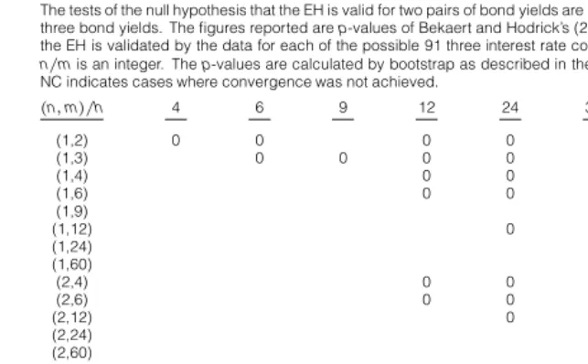
LM Test Statistics: Trivariate VAR
The tests of the null hypothesis that the EH is valid for two pairs of bond yields are performed in a trivariate VAR comprising three bond yields. The figures reported arep-values of Bekaert and Hodrick’s (2001) LM tests of the null hypothesis that the EH is validated by the data for each of the possible 91 three interest rate combinations of our 12 bond yields where n/mis an integer. Thep-values are calculated by bootstrap as described in the text. 0 denotesp-values below 10−4. NC indicates cases where convergence was not achieved.
(n,m)/h 4 6 9 12 24 36 48 60 120
(1,2) 0 0 0 0 0 0 0 NC
(1,3) 0 0 0 0 0 NC NC 0
(1,4) 0 0 0 0 0 0
(1,6) 0 0 0 0 0 NC
(1,9) 0
(1,12) 0 0 0 0 0
(1,24) 0 0
(1,60) NC
(2,4) 0 0 0 0 0 NC
(2,6) 0 0 0 0 0 0
(2,12) 0 0 0 0 0
(2,24) 0 0
(2,60) NC
(3,6) 0 0 0 0 0 0
(3,9) 0
(3,12) 0 0 0 0 0
(3,24) NC NC
(3,60) NC
(4,12) 0 0 0 0 NC
(4,24) 0 NC
(4,60) NC
(6,12) 0 0 0 0 0
(6,24) 0 0
(6,60) NC
(12,24) 0 0
(12,60) NC
term structure—as it is often recorded by the relevant literature—but throughout the maturity spectrum from one-month to 10-year yields.11
We now turn to some Monte Carlo evidence and robustness checks on our core results.
V.
Monte Carlo Evidence and Robustness Checks
In this section, we investigate further our claim that the two tests based on expanded VARs, either with macroeconomic fundamentals or with more than two bond yields, lead to an increase in power relative to the simple bivariate VAR tests. To this end, we conduct Monte Carlo experiments designed to measure the empir-ical power of the three VAR-based LM tests employed in the empirempir-ical analysis. We also report some robustness checks carried out to assess the sensitivity of our core results, presented in Section IV, to the potential presence of structural breaks in the VARs and to the choice of the optimization method used in performing the LM tests.
A. The Empirical Power of the VAR Tests
We calculate the empirical power of the LM tests as the percent of Monte Carlo experiments carried out under the alternative hypothesis that the EH does 11Given the rejections of the EH, the VARs employed in this paper might provide insights on the
not hold where the test statistic exceeds the empirical critical value, calculated by bootstrap as described in Section IV. Table 6 reports the values of the empiri-cal power of the LM tests for the three different VARs considered in this paper. Following Bekaert and Hodrick (2001), we use the unconstrained VAR as the alternative hypothesis.12
TABLE 6
Empirical Power of LM Tests of the EH
The figures denote the empirical power of the LM test statistic when the data are generated under the alternative hypoth-esis, as described in the text, under three different cases. Case 1 relates to a bivariate VAR with two bond yields. Case 2 relates to a bivariate VAR with two bond yields and macroeconomic fundamentals (unemployment rate and inflation rate), and Case 3 relates to a trivariate VAR with three bond yields.
Nominal Level
0.01 0.05 0.10
Case 1 0.648 0.707 0.734
Case 2 0.779 0.820 0.854
Case 3 0.870 0.955 0.981
The LM test calculated from the bivariate VAR with two bond yields (Case 1 in Table 6) displays an empirical power of about 65% at the 1% level, 71% at the 5% level, and 73% at the 10% level. These results are comparable to the empirical power recorded by Bekaert and Hodrick (2001), who report similar empirical power for EH tests.
For the expanded VAR with macroeconomic factors as conditioning infor-mation (Case 2 in Table 6), power increases to about 78% at the 1% level, 82% at the 5% level, and about 85% at the 10% level. This is consistent both with the conjecture that macroeconomic conditioning information enhances the power of the EH tests and with thefindings presented in Section IV.B.
Finally, the highest power is obtained for the VAR with three bond yields (Case 3 in Table 6), where the empirical power is 87% at the 1% level, and about 96% and 98% at the 5% and 10% levels, respectively, for the null hypothesis that the EH holds on two pairs of bond yields. Again, this is consistent both with our priors and with thefinding that the EH is rejected throughout the U.S. yield curve, as reported in Section IV.C. Overall, the Monte Carlo evidence confirms that the two expanded VARs lead to more powerful LM tests.
B. Structural Breaks
Campbell and Shiller (1991) found evidence that the EH performed better during the 1952–1978 sample period than during the entire sample period. To investigate the robustness of the results to the sample period, we test for structural breaks in the VARs using the procedure for endogenous break testing suggested
12Specifically, the results reported were obtained using the unconstrained VAR for bond yields
by Andrews and Ploberger (1994). This procedure is applied to each of the 48 rate combinations for the bivariate VARs.13
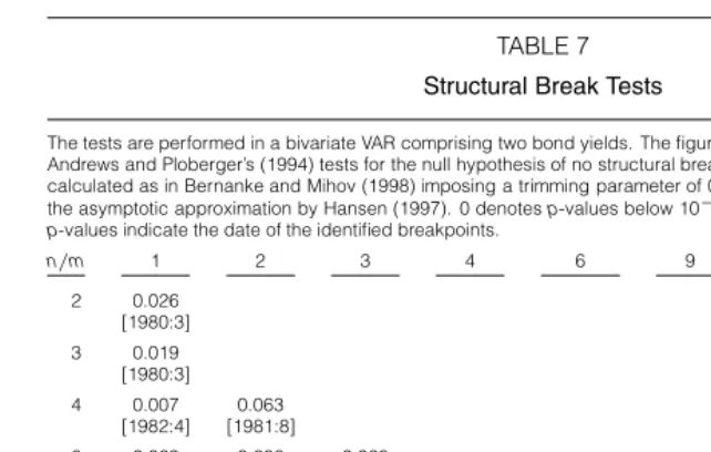
The results, reported in Table 7, suggest a variety of structural breaks that cluster around two periods, 1980–1981 and 1961–1962. Because the qualitative results were relatively insensitive to the specific choice of the break date, the results are presented only for two periods. Thefirst period, 1952:01–1978:12, is consistent with Campbell-Shiller’s argument that the EH may have performed better before 1978 than after. The second period, 1982:01–2003:12, takes into account the finding that the main structural break appears to be around 1980– 1981, which is consistent with a widely held view that the behavior of interest rates may have changed in the early 1980s (e.g., Ang and Bekaert (2002)).14
TABLE 7
Structural Break Tests
The tests are performed in a bivariate VAR comprising two bond yields. The figures reported are the smallestp-values of Andrews and Ploberger’s (1994) tests for the null hypothesis of no structural break at unknown point. The test statistic is calculated as in Bernanke and Mihov (1998) imposing a trimming parameter of 0.15. Thep-values are calculated using the asymptotic approximation by Hansen (1997). 0 denotesp-values below 10−4. Values in square brackets under the p-values indicate the date of the identified breakpoints.
n/m 1 2 3 4 6 9 12 24 60
[image:17.612.61.382.279.483.2]2 0.026
[1980:3]
3 0.019
[1980:3]
4 0.007 0.063
[1982:4] [1981:8]
6 0.020 0.236 0.028
[1981:8] [1981:8] [1980:3]
9 0 0.045
[1981:8] [1980:3]
12 0 0.044 0.050 0.017 0
[1981:8] [1981:8] [1981:8] [1981:8] [1961:10]
24 0 0.006 0.003 0.003 0 0
[1981:8] [1981:8] [1981:8] [1981:8] [1961:10] [1981:8]
36 0 0 0.003 0.002 0 0 0
[1981:8] [1981:8] [1981:8] [1981:8] [1961:10] [1981:8] [1962:2]
48 0 0 0.001 0.001 0 0 0
[1981:8] [1981:8] [1981:8] [1981:8] [1961:10] [1962:2] [1962:2]
60 0 0 0.002 0.002 0 0
[1981:8] [1981:8] [1981:8] [1981:8] [1961:10] [1962:2]
120 0 0.002 0.004 0.002 0 0 0 0
[1981:8] [1981:8] [1981:8] [1981:8] [1961:10] [1962:2] [1962:2] [1981:8]
Thep-values from the LM statistics for the bivariate VARs are presented in Table 8 for both subsamples examined (Panels A–B). The qualitative conclusions about the EH are similar for the two periods. For most interest rate combinations
13Essentially we applied the structural break tests following the same reasoning as Bernanke and
Mihov (1998), p. 889, by examining all possible combinations.
14The three years from 1979:01 to 1982:12 were excluded because of the well-known volatility
where the EH was not rejected in thefirst period, it was also not rejected in the second period. Moreover, the EH is generally rejected at the short end of the maturity spectrum but not at the longer end. However, there is some evidence in favor of the Campbell-Shiller conjecture that the EH performed better in the pre-1978 period since the rejection of the EH in that period is very robust only when the longer rate has maturity of one year or less, whereas in the post-1982 sample period wefind a rejection of the EH that is quite robust when the longer rate has a maturity of two years or shorter. Overall, thesefindings resemble the results for the full sample reported in Table 2.
TABLE 8
LM Test Statistics: Sub-Periods
The tests are performed in a bivariate VAR comprising two bond yields. The figures reported arep-values of Bekaert and Hodrick’s (2001) LM tests of the null hypothesis that the EH is validated by the data for each of the possible 48 combinations of our 12 bond yields wheren/mis an integer. Thep-values are calculated by bootstrap as described in the text. 0 denotesp-values below 10−4. Figures in bold denote cases where the EH is not rejected at the 5% significance level.
n/m 1 2 3 4 6 9 12 24 60
2 0
3 0
4 0 0
6 0 0 0
9 0 0
12 0.012 0 0 0 0.352
24 0.025 0.087 0.097 0.168 0.287 0
36 0.104 0.204 0.201 0.240 0.318 0.042 0.028
48 0.164 0.170 0.304 0.344 0.425 0.207 0.064 60 0.233 0.384 0.347 0.392 0.497 0.041
120 0.284 0.495 0.298 0.351 0.368 0.184 0.037 0.021
2 0
3 0
4 0 0
6 0 0 0
9 0 0
12 0 0 0 0 0
24 0.015 0.037 0.017 0.018 0.012 0
36 0.122 0.214 0.113 0.124 0.118 0.102 0.083
48 0.254 0.370 0.304 0.192 0.235 0.012 0.040 60 0.383 0.419 0.470 0.392 0.417 0.144
120 0.780 0.750 0.710 0.692 0.860 0.061 0.087 0.122 Panel A. 1952:01–1978:12 Sample Period
Panel B. 1982:01–2003:12 Sample Period
While Table 8 reports the subsamples results only for the bivariate LM test with two bond yields, we also performed the subsample analysis on the LM tests for the expanded VAR with macroeconomic fundamentals and with three bond yields for some of the rate combinations considered. For the rate combinations examined, the results across the two subsamples were consistent with the full sample results in Tables 4–5.
C. Optimization Method and Convergence
and the Davidon-Fletcher-Powell (DFP) methods. The Newton method did not converge in 55 cases whereas the DFP method did not converge in 19 of the 91 cases examined. In all cases where the two alternative procedures converge, the EH is rejected.
Also, in Section IV.C we interpret non-convergence as a possible rejection of the EH. In this regard, it is interesting to note that in the eight instances where the DFP method converged when the BFGS method did not, the EH is rejected with a very lowp-value. These results are consistent with our suggestion in Section IV.C that non-convergence may be due to the unrestricted VAR coefficients being “too far” from any set of coefficients that satisfy the EH. Of course, these re-sults do not prove that non-convergence implies a rejection of the EH constraints since non-convergence may be caused by factors other than large violations of the constraints.15
VI.
Conclusions
The EH plays important roles in economics andfinance and, not surprisingly, has been widely tested using a variety of tests and data. Our paper extends this literature by testing the restrictions implied by the EH on a VAR of the long- and short-term rate using the Lagrange multiplier test recently proposed by Bekaert and Hodrick (2001). The VAR test rejects the EH at the shorter end of the ma-turity spectrum (when the long rate is two years or shorter), but not at the longer end, consistent with the mixed results often recorded in the relevant literature (Campbell and Shiller (1987), (1991)).
In order to increase the test power, we extended the analysis in two direc-tions. First, inspired by the growing literature linking macroeconomic funda-mentals to the behavior of the term structure of interest rates, we investigate the possibility of increasing test power by expanding the VAR model to allow macroe-conomic variables as conditioning information. Second, we increase the size of the VAR by using more than two yields and testing the EH on more than one pair of rates. Our results are less encouraging for the EH when the interaction between the term structure and the macroeconomy is considered and when the VARs are extended to include more than two bond yields. When the relation between the term structure and the unemployment and inflation rates is accounted for, the EH is rejected in nearly all cases when the longer rate has a maturity of four years and in all cases when the longer rate is three years or shorter. In addition, for the model with three bond yields either the EH is strongly rejected at very low marginal significance levels or the procedure fails to converge. In addition, the increase in test power obtained from conditioning on macroeconomic variables and from including more than two bond yields is supported by a Monte Carlo analysis that suggests that empirical power is higher for the expanded VARs.
The evidence in this paper confirms the usefulness of the recently developed testing procedure proposed by Bekaert and Hodrick (2001) and the potential to enhance its power properties by extending the underlying models to allow for
15We are thankful to James McCulloch, Roel Oomen, and Mark Salmon for a useful conversation
macroeconomic factors or several interest rates. More importantly, our empirical results suggest that departures from the EH of the term structure of interest rates are statistically important and pervasive throughout the U.S. yield curve from one-month to 10-year rates. This may be due to various reasons, including the violation of the assumption of a constant risk premium underlying the EH and the possibility that the models we use, albeit richer than many others examined in the literature, may still provide a poor approximation to the potentially much more complex process that drives the term structure of interest rates. Much more work needs to be done to understand the term structure of bond yields. The evidence presented here suggests that the term structure is likely to be considerably more complex than the EH suggests.
References
Andrews, D. W. K. “Heteroskedasticity and Autocorrelation Consistent Covariance Matrix Estima-tion.”Econometrica, 59 (1991), 817–858.
Andrews, D. K. W., and W. Ploberger. “Optimal Tests When a Nuisance Parameter Is Present Only Under the Alternative.”Econometrica, 62 (1994), 1383–1414.
Ang, A., and G. Bekaert. “Regime Switches in Interest Rates.” Journal of Business and Economic Statistics, 20 (2002), 163–182.
Ang, A., and M. Piazzesi. “A No-Arbitrage Vector Autoregression of Term Structure Dynamics with Macroeconomic and Latent Variables.”Journal of Monetary Economics, 50 (2003), 745–787. Ang, A.; M. Piazzesi; and M. Wei. “What Does the Yield Curve Tell Us about GDP Growth?” Mimeo,
Columbia University and University of Chicago (2003).
Bansal, R., and H. Zhou. “Term Structure of Interest Rates with Regime Shifts.”Journal of Finance, 57 (2002), 1997–2043.
Bekaert, G.; S. Cho; and A. Moreno. “New-Keynesian Macroeconomics and the Term Structure.” Mimeo, Columbia University (2004).
Bekaert, G., and R. J. Hodrick. “Expectations Hypotheses Tests.” Journal of Finance, 56 (2001), 1357–1394.
Bekaert, G.; R. J. Hodrick; and D. A. Marshall. “On Biases in Tests of the Expectations Hypothesis of the Term Structure of Interest Rates.”Journal of Financial Economics, 44 (1997), 309–348. Bekaert, G.; M. Wei; and Y. Xing. “Uncovered Interest Rate Parity and the Term Structure.” Mimeo,
Columbia University (2004).
Bernanke, B. S., and I. Mihov. “Measuring Monetary Policy.”Quarterly Journal of Economics, 113 (1998), 869–902.
Bliss, R. R. “Testing Term Structure Estimation Methods.” Advances in Futures and Options Re-search, 9 (1997), 197–231.
Campbell, J. Y., and R. J. Shiller. “Cointegration and Tests of Present Value Models.” Journal of Political Economy, 95 (1987), 1062–1088.
Campbell, J. Y., and R. J. Shiller. “Yield Spreads and Interest Rate Movements: A Bird’s Eye View.”
Review of Economic Studies, 58 (1991), 495–514.
Carriero, A.; C. A. Favero; and I. Kaminska. “Financial Factors, Macroeconomic Information and the Expectations Theory of the Term Structure of Interest Rates.” Journal of Econometrics, 131 (2006), 339–358.
Clarida, R. H.; L. Sarno; M. P. Taylor; and G. Valente. “The Role of Asymmetries and Regime Shifts in the Term Structure of Interest Rates.”Journal of Business, 79 (2006), 1193–1224.
Dewachter, H., and M. Lyrio. “Macro Factors and the Term Structure of Interest Rates.”Journal of Money, Credit and Banking, 38 (2006), 119–140.
Diebold, F. X.; G. D. Rudebusch; and S. B. Aruoba. “The Macroeconomy and the Yield Curve: A Dynamic Latent Factor Approach.”Journal of Econometrics, 131 (2006), 309–338.
Elliott, G.; J. H. Stock; and T. J. Rothenberg. “Efficient Tests for an Autoregressive Unit Root.”
Econometrica, 64 (1996), 813–836.
Engsted, T., and C. Tanggaard. “Cointegration and the U.S. Term Structure.”Journal of Banking and Finance, 18 (1994), 167–181.
Frankel, J. A., and K. A. Froot. “Using Survey Data to Test Standard Propositions Regarding Ex-change Rate Expectations.”American Economic Review, 77 (1987), 133–153.
Froot, K. A. “New Hope for the Expectations Hypothesis of the Term Structure of Interest Rates.”
Journal of Finance, 44 (1989), 283–305.
Greene, W. H.Econometric Analysis, 4th ed. New York, NY: Prentice Hall (2000).
Gurkaynak, R. S.; B. Sack; and E. Swanson. “The Sensitivity of Long-Term Interest Rates to Eco-nomic News: Evidence and Implications for MacroecoEco-nomic Models.” American Economic Re-view, 95 (2005), 425–436.
Hall, A. D.; H. M. Anderson; and C. W. J. Granger. “A Cointegration Analysis of Treasury Bill Yields.”Review of Economics and Statistics, 74 (1992), 116–126.
Hamilton, J. D.Time Series Analysis. Princeton, NJ: Princeton University Press (1994).
Hansen, B. E. “Approximate Asymptotic P-Values for Structural Change Tests.”Journal of Business and Economic Statistics, 15 (1997), 60–67.
Hansen, L. P. “Large Sample Properties of Generalized Method of Moments Estimators.” Economet-rica, 50 (1982), 1029–1054.
Kool, C. J. M., and D. L. Thornton. “A Note on the Expectations Theory and the Founding of the Fed.”Journal of Banking and Finance, 28 (2004), 3055–3068.
Kozicki, S., and P. A. Tinsley. “Shifting Endpoints in the Term Structure of Interest Rates.” Journal of Monetary Economics, 47 (2001), 613–652.
Kwiatkowski, D.; P. C. B. Phillips; P. Schmidt; and Y. Shin. “Testing the Null Hypothesis of Station-arity against the Alternative of a Unit Root: How Sure Are We That Economic Time Series Have a Unit Root?”Journal of Econometrics, 54 (1992), 159–178.
McCulloch, H. J., and H.-C. Kwon. “U.S. Term Structure Data, 1947–1991.” Ohio State University Working Paper No. 93-6 (1993).
Rudebusch, G. D., and T. Wu. “A Macro-Finance Model of the Term Structure, Monetary Policy, and the Economy.” Federal Reserve Bank of San Francisco Working Paper 2003-17 (2004).
Sarno, L., and D. L. Thornton. “The Dynamic Relationship between the Federal Funds Rate and the Treasury Bill Rate: An Empirical Investigation.” Journal of Banking and Finance, 27 (2003), 1079–1110.
Shiller, R.; J. Y. Campbell; and K. L. Schoenholtz. “Forward Rates and Future Policy: Interpreting the Term Structure of Interest Rates.”Brookings Papers on Economic Activity, 1 (1983), 173–217. Sims, C. A. “Macroeconomics and Reality.”Econometrica, 48 (1980), 1–48.
Stock, J. H., and M. W. Watson. “Testing for Common Trends.” Journal of the American Statistical Association, 83 (1988), 1097–1107.
Stock, J. H., and M. W. Watson. “Forecasting Inflation.”Journal of Monetary Economics, 44 (1999), 293–335.
Thornton, D. L. “Tests of the Expectations Hypothesis: Resolving Some Anomalies When the Short-Term Rate is the Federal Funds Rate.”Journal of Banking and Finance, 29 (2005), 2541–2556. Thornton, D. L. “Tests of the Expectations Hypothesis: Resolving the Campbell-Shiller Paradox.”
Journal of Money, Credit, and Banking, 38 (2006), 511–542.
Waggoner, D. F. “Spline Methods for Extracting Interest Rate Curves from Coupon Bond Prices.”