University of Warwick institutional repository: http://go.warwick.ac.uk/wrap
This paper is made available online in accordance with
publisher policies. Please scroll down to view the document
itself. Please refer to the repository record for this item and our
policy information available from the repository home page for
further information.
To see the final version of this paper please visit the publisher’s website.
Access to the published version may require a subscription.
Author(s): Higgins, M.D. Green, R.J.and Leeson, M.S.;
Article Title: A Genetic Algorithm Method for Optical Wireless Channel
Control
Year of publication: 2009
Link to published article:
http://dx.doi.org/
10.1109/JLT.2008.928395
Publisher statement:
“© 2009 IEEE. Personal use of this material is
permitted. Permission from IEEE must be obtained for all other uses, in
any current or future media, including reprinting/republishing this
material for advertising or promotional purposes, creating new
collective works, for resale or redistribution to servers or lists, or reuse
of any copyrighted component of this work in other works.”
A Genetic Algorithm Method for Optical Wireless
Channel Control
Matthew D. Higgins, Roger J. Green,
Senior Member, IEEE,
and Mark S. Leeson,
Senior Member, IEEE
Abstract—A genetic algorithm controlled multispot transmitter is proposed as an alternative approach to optimising the power distribution for single element receivers in fully diffuse mobile indoor optical wireless communication systems. By specifically tailoring the algorithm, it is shown that by dynamically altering the intensity of individual diffusion spots, a consistent power distribution, with negligible impact on bandwidth and rms delay spread, can be created in multiple rooms independent of reflectivity characteristics and user movement patterns. This advantageous adaptability removes the need for bespoke system design, aiming instead for the use of a more cost effective, optimal transmitter and receiver capable of deployment in multiple scenarios and applications. From the simulations conducted it is deduced, that implementing a receiver with a FOV= 55◦
in conjunction with either of two notable algorithms, the dynamic range of the rooms, referenced against the peak received power, can be reduced by up to26%when empty, and furthermore to within12%of this optimised case when user movement perturbs the channel.
Index Terms—Genetic algorithm, optical communication, wire-less LAN.
I. INTRODUCTION
O
NE of the most challenging design aspects of an indoor optical wireless (OW) system, using an infrared (IR) carrier, is overcoming the limitations imposed by the transmis-sion channel. Conventional diffuse configurations, pioneered by Gfeller [1], suffer from intersymbol interference (ISI), wide ranging levels of received power throughout the room and intense quantities of IR ambient radiation [2]. These channel characteristics inhibit the ability to provide high performance OW systems that meet the needs of today’s growing demand for mobile multimedia device connectivity. Furthermore, the transmission channel characteristics are dependent upon the room size, stationary and moving objects, material properties of every surface the radiation is incident upon, and the number and type of illumination sources present [3], such that a single system design may have different performance capabilities when implemented in different locations.To overcome these performance issues, research in the field has led to several possible solutions. Quasi-diffuse configu-rations employing multispot diffusion (MSD) and diversity receivers [4] improve the bandwidth and ambient noise rejec-tion through the use of an array of photodetector’s coupled to either, a single imaging lens [5], or several optical concentra-tors [6]. Implementation of automatic gain control (AGC) can
The authors are with the Department of Engineering, University of War-wick, Coventry, CV4 7AL, UK.
E-mail:{m.higgins, roger.green, mark.leeson}@warwick.ac.uk Manuscript received October 5, 2007. Revised April 4, 2008.
compensate for the variations in received power at different positions within the room [7]. Modulation techniques such as trellis-coded pulse-position modulation [8], and amplitude shift key digital demodulation [9] are capable of mitigating the effects of ISI, and noise from fluorescent lamps, respectively. More recently the use of intelligent techniques have been shown to be beneficial, using neural networks and pattern recognition wavelet analysis to overcome channel induced distortion [10]. Following this, a modified genetic algorithm (GA), based on simulated annealing [11], has been shown to produce highly optimised computer generated holograms, reducing the variation in received power distribution [12], [13]. The most practical OW system architecture is the cellular approach, where a given room has a transceiver base station linked to the backbone network. It is presumed that there are multiple end users in the cell, each with a battery powered portable OW receiver, such as mobile phone, laptop or PDA. Therefore whilst the application of each of the aforementioned techniques has respective performance merits compared to a conventional diffuse OW system, one has to weigh these benefits against the added complexity, cost and physical size of each receiver within the system. This is especially apparent when the number of receivers becomes large, as the cost overhead of a system, will be influenced more by the number of receivers, than the single base station.
In this paper a GA controlled MSD transmitter is proposed, but instead of pairing it with a diversity receiver, a simpler single element receiver is implemented. It will be shown that the GA can dynamically optimise the power distribu-tion for multiple stadistribu-tionary and mobile users within multiple environments, by controlling the power of each diffusion spot. This advantageous adaptability, independent of environ-mental characteristics and user movement patterns, removes the need for bespoke system design and allows for easier system deployment increasing end user friendliness. Moreover the ability to produce a consistent power distribution at all locations within multiple environments contributes towards uniform system performance characteristics. These perfor-mance characteristics then become less dependent upon the ACG capabilities of the receiver, as the transmitter becomes responsible for maximising the signal to noise ratio (SNR) and data rate. The inevitable trade off in the work presented here is the lack of substantial bandwidth gains compared to implementing diversity receivers, but in applications where mobility and cost are paramount, this method aid in the design of an optimum, standardised receiver design realisable for mass product integration.
II briefly overviews the general system model, applicable transmitter techniques, and impulse response definitions. Sec-tion III introduces the channel model theory followed by sec-tion IV detailing the GA implementasec-tion. Secsec-tion V provides the results and associated analysis of using the proposed GA. Concluding remarks are presented in section VI.
II. SYSTEMMODEL
A. Source, Receiver and Reflector Model
We define our system environment to be an arbitrary indoor rectangular room enclosing a transmitter capable of firstly forming a diffusion spot geometry upon the ceiling and secondly, that each spot intensity can be dynamically and in-dependently controlled. To the best of the authors’ knowledge, holographic diffusers [14], whilst being capable of generating predefined spot intensities and/or geometries, such as uniform, diamond or line-strip [15], have static characteristics removing its suitability for the work presented here.
Multiple optical sources [16] allow for any spot pattern geometry to be installed on the ceiling of the room, and whilst it is possible to control the distribution of emitted radiation from each source though the use of lenses or other diffuser techniques [17], traditionally the optical source is a LED, which emits radiation with a generalised Lambertian radiation intensity pattern [18]. Dynamic control of an individual spot intensity is also possible. The installation of multiple optical sources may seem ‘bespoke’, but the use of white LEDs which not only act as transmission sources, also serve to illuminate the environment, and have beneficial properties such as low power consumption, heat dissipation and cost.
A 2-D vertical cavity surface emitting Laser diode (VCSEL) or resonant cavity LED (RCLED) array, flip-chip bonded to CMOS driver circuitry, allows for a highly-integrated trans-mitter solution [19], [20]. The driver circuitry is capable of controlling each element’s emitted power, along with any other signal processing techniques currently realisable in CMOS. Furthermore, it is possible to integrate beam shaping and steering optics, that can control the position of each of the resultant projected spots on the ceiling, which will then be reflected, according to the reflection properties of the ceiling. Assuming that the majority of surfaces in our environment exhibit a fully diffuse, as supposed to specular [21]–[23], reflection characteristic that can be described by Lambert’s reflection model [24], we can apply the following simpli-fication. Regardless of whether the transmitter is composed of multiple optical sources or a 2-D VCSEL/RCLED array, the resultant diffusion spots on the ceiling will exhibit a Lambertian radiation intensity pattern, and therefore from this point onwards, each of theIdiffusion spots on the ceiling will themselves be considered independent sources Si. The only error induced with this assumption is a delay and propagation loss between the emitting element of an 2-D VCSEL/RCLED array and the diffusion spot position. In an arbitrary room, the number of possible transmitter and diffusing spot positions is essentially infinite, and so this assumption also serves to simplify our argument for using the GA whilst maintaining generality to the application. Referring to figure 1, each source
Si will therefore have an associated position vector rS
i, unit length orientation vector nˆS
i, power PSi and uniaxial symmetric, with respect tonˆS
i, Lambertian radiation intensity profileR(φ)given by
R(φ) = n+ 1
2π PSicos
n(φ)
for θ∈[−π/2, π/2] (1) Where the mode number,n= 1for a pure Lambertian diffuser, such as the ceiling, andn >1 for a diffusion pattern from an LED with higher directionality.
The aim of this work is to control the power distribution of radiation, enabling the use of a single optimal receiver design at all locations in multiple locations. Therefore, for a given environment we model the existence ofJ single element receivers Rj. Knowing that receivers Rj and Rj+1 are of
the same design, we can simultaneously simulate and readily interchange between describing a system with J receivers at multiple locations and a system with one receiver at J
locations. To attain a highly detailed system model, we set
J = 1024 and uniformly distributed the position vectorsrR
j of the receivers Rj over the width x, length y, at a height
z= 1m. Each receiver has a vertical orientation vector nˆR
j, active optical collection areaARj and a field of viewF OVRj defined as the maximum uniaxial symmetric incident angle of radiation with respect to nˆR
j, that will generate a current in the photodiode. As we have assumed all surfaces within the environment exhibit Lambertian reflection characteristics, which are independent of the angle of the incident radiation, we follow the technique described in [25], and partition all surfaces intoLelementsElwith positionrE
l, orientationnˆEl, and sizeAEl = 1/∆A
2(m2)where∆Ais the desired number
of elements per meter. A given element will sequentially behave, firstly as a receiverER
l with a hemispherical FOV, for which we can determine the received powerPEl, and secondly as a sourceES
l , with a radiation intensity profileR(φ)is given by (1) setting n = 1 and PSi = ρElPEl, where ρEl is the reflectivity of the element.
B. Impulse Response Calculations
The IR radiation incident upon a receiver Rj will be the result of the radiation emitted from a sourceSi that has prop-agated directly through an unobstructed LOS path, and/or from the radiation that has undergone a finite number,k, reflections off the surfaces within the environment. It is also known [24], [25] that, for an intensity modulation, direct detection (IM/DD) channel, where the movement of transmitters, receivers or objects in the room is slow compared to the bit rate of the system, no multipath fading occurs, and, as such, can be deemed an LTI channel. The impulse response h(t;Si,Rj) is given by [25], [26]
h(t;Si,Rj) = k
X
k=0
hk(t;S
i,Rj) (2)
wherehk(t;S
i,Rj)is the impulse response of the system for radiation undergoingk reflections betweenSi andRj.
To determine the impulse response, we assume our source
Rj,ElR
Si,ElS
ˆ n{S
i,ElS}
ˆ n{R
j,ERl} φ
θ
FOVRj R(φ)
D n= 50
n= 3
n= 1
A{Rj,ER
l }
r{R
j,ElR}
r{S
[image:4.595.60.287.112.304.2]i,ElS}
Fig. 1. Source, receiver and reflector geometry, adapted from [25]
the LOS (k= 0)impulse response is given by the scaled and delayed Dirac delta function
h0(t;Si,Rj)≈R(φij)
cos(θij)ARj
Dij
V( θij
FOVRj
)δ(t−Dij
c )
(3) Where, referring to figure 1,Dij =||rS
i−rRj||is the distance between source and receiver, c is the speed of light. φij and
θij are the angles betweennˆS
i and(rRj −rSi)and between
ˆ
nR
j and (rSi −rRj) respectively. V(x) represents the the visibility function, whereV(x) = 1for|x| ≤1, andV(x) = 0
otherwise.
For radiation undergoing k > 0 bounces, the impulse response is given by
hk(t;S
i,Rj) = L
X
l=1
h(k−1)(t;S
i,ElR)∗h0(t;ElS,Rj) (4) Where∗denotes convolution, and thek−1 impulse response
h(k−1)(t;S
i,ElR)can be found iteratively [26] from
hk(t;S
i,ElR) = L
X
l=1
h(k−1)(t;S
i,ElR)∗h0(t;ElS,ElR) (5) Where all the zero order (k = 0), responses in (4) and (5) are found by careful substitution of the variables in (3). The computational time required for calculation of the impulse response using this iterative method is proportional to k2 [27], and we will firstly limit ourselves to the a third
order impulse response (k = 3), and secondly change the segmentation resolution of the environment for each reflection, setting∆A1= 20,∆A2= 6and∆A3= 2. It should also be
noted that the resultant impulse response in (2) will result in the finite sum of scaled delta functions which need to undergo temporal smoothing by subdividing time into bins of width∆t, and summing the total power in each bin [25]. For this work, we assume a single time bin width of∆t= 0.1ns.
III. THECHANNELMODEL
A. Scaling Factors
For a nondirected IR channel employing IM/DD, a source
Si which emits an instantaneous optical power Xi(t), will produce a instantaneous photocurrent Yij(t) at receiver Rj with photodiode responsivityrj, in the presence of an additive, white Gaussian shot noise Nj(t), and can modelled as the linear baseband system given by [28]
Yij(t) =rjXi(t)∗h(t;Si,Rj) +Nj(t) (6) Whereh(t;Si,Rj)is the impulse response given by (2), and is fixed for a given system configuration ofSi andRj.
Assuming that all I sources Si emit an identical signal waveform, such that X1(t) = X2(t) = . . . = XI(t), but whose magnitude is individually scaled by a factor ai, the instantaneous photocurrent generated at a given receiverYj(t) is simply the summation of (6) for all
sources:-Yj(t) = I
X
i=1
(rjaiXi(t)∗h(t;Si,Rj)) +Nj(t) (7) Furthermore, as we are only concerned with a single re-ceiver design, the photodiode responsivity rj is constant for each receiver or receiver location, such that there may exist a set ofIscaling factorsai, that can be applied to theIidentical signal waveformsXi(t), that will allow for theJ receivers, to attain the same or very similar instantaneous photocurrents
Y1(t)≈Y2(t)≈. . .≈YJ(t) (8)
Knowing that the channel is linear we can rewrite (7) as
Yj(t) = I
X
i=1
(rjXi(t)∗aih(t;Si,Rj)) +Nj(t) (9) Such that we can solve (8) by solving
I
X
i=1
aih(t;Si,R1) ≈
I
X
i=1
aih(t;Si,R2)≈. . .
. . .≈
I
X
i=1
aih(t;Si,RJ) (10) By inspection of equations (7) to (10), it can be seen that a solution may require some scaling factors of≤1, lowering the total received power, compared to if all sources were the same. Furthermore solving (8) for different environments, will yield non-identical sets of scaling factors implying the magnitude of received power, although equal at all locations within, will be different.
compared to a conventional point source. The same logic can also be applied when using multiple LEDs, as they have a larger diameter than a point source. Whilst the GA will adapt the power of each diffusion spot, the system must still be within the AEL at the worst case of all spots at maximum.
Drawing parallels with the IEEE 802.11a WiFi physical layer specification, that incorporates multi-rate transmission of up to 54Mbit/s [31], and recent work on rate-adaptive transmission [32] in the IR domain, if it is found that several environments have different received powers the following method can be applied. Firstly by normalising the I scaling factors, the equality result of (8) is independent of receiver power magnitude, and secondly for different environments we can adjust for example, the pulse characteristic, in order to increase or decrease the received power to make the power distributions equal. This then allows for the same optimal receiver design to be used in different environments, albeit under the compromise of variable data rates in the same manner as most other variable data rate systems.
To illustrate the final problem simplification we have ap-plied, consider for example an environment such as config-uration A in [25], with dimensions x = 5m, y = 5m, z = 3m. In calculating a third order reflection impulse response
(k = 3), the longest time of flight for the radiation to travel ist= (4(52+ 52+ 32)0.5)/c≈102.4ns, when it undergoes a
path reflecting off the opposite corners of the room. Using an impulse response bin width ∆t= 0.1ns, would produce1024
samples for each impulse response train, for every combination of I sources andJ receivers in (10).
In the general case, proposing a GA that can solve (10) for the possibly infinite number of source and transmitter configurations would prove to be too unwieldy. By replacing the need to evaluate each bin of the impulse response train, with the need to find only the scaling factor solution for the time integral or the DC value of the frequency response
H(0;Si,Rj) =
R∞
−∞h(t;Si,Rj)dt, equation (10) reduces to I
X
i=1
aiH(0;Si,R1) ≈
I
X
i=1
aiH(0;Si,R2)≈. . .
. . .≈
I
X
i=1
aiH(0;Si,RJ) (11) The power distribution optimisation should not be achieved at the expense of bandwidth and rms delay spread. As (11) only quantifies the total power received, not when the power was received we will feed back the solution into the original system model to quantify our worst case bandwidth and rms delay spread, defined as the smallest and largest values at any location within the room respectively. The rms delay spread can be found from the original impulse response using [33]
σ=
v u u t
R∞
−∞(t−ω)2h2(t)dt
R∞
−∞h2(t)dt
(12)
Whereω is defined as:
ω=
R∞
−∞th
2(t)dt
R∞
−∞h2(t)
(13)
IV. THEGENETICALGORITHM
GAs should not be considered off-the-peg, ready to use algorithms, but rather a general framework that needs to be tailored to a specific problem [34]. Below we describe our methodology and justifications for decisions made in adapting the representation, fitness function, selection, recombination and mutation routines found in a so-called canonicalGA.
A. Representation
The genotype represents all the information stored in the chromosome and allows us to describe an individual at the level of the genes. Our aim is to find a set of scaling factors that can be used to solve (11), such that if we allow ai∀i ∈
{1, . . . , I} to take on a value in the set {0,0.01, . . . ,1}, we can define our genotypic search spaceΦg={0,0.01, . . . ,1}I, which will provide |Φg| = 101I possible solutions [35]. We further define a populationΨ(t)at timet, ofµchromosomes
aν = (a1, . . . , aI)∈Φg,∀ν ∈ {1, . . . , µ} which provide our
basic representation of a possible solution in a form that can be operated on by the GA. The initial population of chromosomes is formed by a uniform pseudo random number generator capable of only generating numbers in the set{0,0.01, . . . ,1}, such that the larger the population the better the chance of an initialisation with a uniform distribution of possible solution values. However, this would also require a larger memory overhead on the hardware implementation, and so we need to find the smallest population size that will not adversely affect the GAs performance when some ratios are not initialised, and subsequently cannot be evaluated as a possible solution. We will therefore evaluate population sizesµ={50,100,200}.
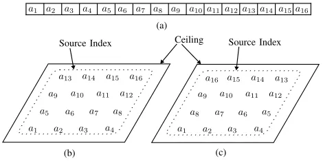
We are also going to investigate what is known as chromo-some epistasis, which refers to a problem-dependent condition in the genotype structure where genes are highly interdepen-dent, such that a good solution may only be found when the value of the genes occur in a particular pattern [36]. Consider for example a system withI= 16, such that our chromosome will contain16scaling factors as in figure 2(a), which translate to the sources on the ceiling in two ways depending upon how we define our genotype structure G. Implementing a wrap-around, (G = WA) structure the scaling factors translate to their respective sources as in figure 2(b), and it can be seen that scaling factorsa4anda5,a8anda9etc. are physically far apart
in application, but adjacent in the chromosome. Alternatively, a concertina (G=CON) structure as in figure 2(c), now shows this problem is alleviated, but other scaling factors, such as
a1 and a8, are now physically close, whilst further apart in
the chromosome. We will test for this condition by applying identical GAs for each genotype structure.
B. The Fitness Function
a1 a1 a1 a2 a2 a2 a3 a3 a3 a4 a4 a4 a5 a5 a5 a6 a6 a6 a7 a7 a7 a8 a8 a8 a9 a9 a9 a10 a10 a10 a11 a11 a11 a12 a12 a12 a13 a13 a13 a14 a14 a14 a15 a15 a15 a16 a16 a16 (b) (c) (a) Ceiling
[image:6.595.59.294.105.222.2]Source Index Source Index
Fig. 2. Chromosome epistasis. (a) Chromosome structure. (b) Wrap around genotype structure. (c) Concertina genotype structure.
only the genotypic properties which still require evaluation at the level of the phenotype [35]. This evaluation is commonly known as the fitness, or objective function, F, which, for the results presented here, is given by
F(aν) = 100−
100
maxH(0;
aν)−minH(0;aν)
maxH(0;aν)
(14) Where maxH(0;aν) and minH(0;aν) are the maximum
and minimum DC frequency responses at any receiver in the environment after application of the scaling factors aν to
the source powers, respectively. It can be seen that we are measuring the percentage change or deviation from the peak power in the room, for an individualaν, whose source scaling
factors will produce a perfectly uniform power distribution within the room and will have a fitness of100%. Furthermore, we can define our global maximum optimal solution ˆaν to be
ˆ
aν= max
aν∈Φg
F(aν) (15)
In general the choice of a fitness function is one of the more difficult steps in constructing an optimal GA, as the decision is not only problem specific but inherently dependent upon the genotype representation used. Therefore whilst we have applied, for the reasons given in section III-A, a normalised fitness function, based upon a maximum and minimum values of the power deviation, it would be theoretically feasible to use any of a number of mathematical measures, such as mean deviation, provided it fits within the users overall GA structure.
C. Selection
The primary objective of the selection operator is to em-phasise the fitter solutions, with either an explorative or exploitative bias, such that their genotypic information is passed onto the next generation [37]. We implement three selection routines in this work namely, roulette, stochastic uniform sampling (SUS) [38] and tournament selection.
The roulette and SUS selection schemes assign a probability of selection proportional to an individual’s relative fitness within the population, such that an individual’s probability of selection, ppropν , is given by
pprop
ν =
F(aν)
Pµ
ν=1F(aν)
(16)
These probabilities are then contiguously mapped onto a wheel, such thatPµ
ν=1p
prop
ν = 1. A uniform random number is then generated in the interval [0,1], and the individuals whose cumulative probability within the population that spans the number is chosen. The process is repeated µtimes, until a new population has been selected. The roulette wheel is unbiased but suffers from a possible infinite spread, in that statistically any member of the population withppropν >0 can be chosenµtimes for the next generation. SUS overcomes this by generatingµuniformly spaced numbers in the range[0,1], and applying a single randomly generated offset value, that moves the position of the numbers such that each individual is still selected based upon its cumulative probability position relative to others in the population. It thus maintains zero bias, but now it is not possible for a given individual to be chosen beyond its expected number [38].
Tournament selection is carried out by first ranking all members in the population Ψ(t) = {a1, . . . ,aµ} by their
absolute fitness in the populationF(aν), wherea1is the fittest,
andaµ is the least. Then, by randomly selectingq members,
we choose the best for the next generation. The probability of a memberaν being selected is given by [37]
ptorn
ν =
1
µq ((µ−ν+ 1) q
−(µ−ν)q) (17) Increasing the size of the tournamentqincreases the selective pressure, giving fitter members of the population a higher probability of selection. With our chosen population sizes, we can expect that, as we are going to implement tournament selection withq = 2 andq = 3, we will lose approximately
40% and 50% of the genetic material, respectively, through the selection process alone [39]. This gives rise to a very exploitative algorithm, but it looses genetic diversity and risks finding a non optimal solution. However, as tournament selection does not require proportional fitness assignments as in (16), the algorithm operates faster. As previously mentioned the size of the population will dictate hardware memory requirements, but for a mobile applications the speed of the algorithm equates to adaptive latency, vital to usability of the system for both receivers within, entering or leaving the room.
D. Reproduction
Crossover imitates the principles of natural reproduction, and is applied with a probability of ρc to randomly selected individuals chosen by the selection routine. Its purpose is to form new individuals for the next generation which have some parts of the genotypic information as their parents. For this work we apply a single point m = 1 and double point
E. Mutation
Mutation was originally developed as a background operator [34], able to introduce new genetic material into the search routine such that the probability of evaluating a string in
Φg will never be zero. Thus it would still be possible to recover good genetic information that may have been lost through selection [35]. Unlike the crossover operator, mutation is seen as a local search method, because it can only modify elements of an individual, perturbing its genetic information in a much smaller way than crossover, which allows the combining of genotypic information from different parents. As we are going to evaluate different selection routines, we will apply the mutation operator to each gene in each individual with varying probabilities ρm={0,0.05,0.1,0.2}, such that when a random number is generated that is less than the chosen probability, we replace that gene with a new randomly-generated value in the set{0,0.01, . . . ,1}. We will attempt to find the highest possible value aiding in the search, but not too high that we encounter what is know as mutation interference defined as when the mutation rate is so high that solutions are so frequently or drastically mutated that the algorithm never manages to explore any region of the search space thoroughly as good solutions, rather than being formed by mutation, are rapidly destroyed [36].
F. Feedback, Termination and Repeatability
Some feedback loop must exist that passes back information regarding the effectiveness of a solution at each generation. Presently the simulation will simply return the DC gain at each receiver location to the fitness function. In a practical system we envisage two methods. Firstly that the receiver, or more precisely transceiver, returns the DC gain or SNR using a supervisory audio tone similar to GSM techniques, or secondly if this optimisation process has been simulated on many scenarios, and the best and worst case powers are known, the transceiver could simply return a ‘too high’ or ‘too low’ command, informing the transmitter some change should be made to the ratios. Either method could be applied as and when needed, or within some predefined protocol space, and would be suitable when one or many receivers are present. Moreover, both methods are applicable when users enter or leave the room, since in theory, they too have the same receiver design that requires the same power distribution to operate.
In general, a GA is run over many generations until the algorithm converges or the result has satisfied some defined solution criteria. As we were unaware of what the minimum power deviation for a given room will be, we decided upon
[image:7.595.311.561.108.405.2]5000 generations, as this was a reasonable compromise be-tween computational effort, and allowing the algorithm to search for better solutions. As will be shown in section V, all GAs (that would converge) converged within this time frame. Due to the stochastic nature of the GA, for each simulation the results were inevitably slightly different, meaning that to allow presentation of results that are both representative of the GAs performance and repeatable for the reader to follow, we conducted each simulation30times, such that each
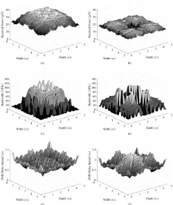
Fig. 3. Empty algorithm test room power, bandwidth and rms delay spread distributions. (a) Non optimised power distribution. (b) Optimised power distribution. (c) Non optimised bandwidth distribution. (d) Optimised bandwidth distribution. (e) Non optimised rms delay spread distribution. (f) Optimised rms delay spread distribution.
performance value presented within section V is the average and the associated standard deviation after the30 retrials.
V. RESULTS
A. Algorithmic Properties
To begin to understand how the GA optimisation would perform, we began by simulating the impulse response of the empty algorithm test room similar to configuration A in [25], with width x = 5m, depth y = 5m and height z = 3m, each wall and ceiling having a reflectivity ρ = 0.8, and the floor having a reflectivity of ρ = 0.3. 16 sources were uniformly distributed over the ceiling, orientated towards the floor, with a Lambertian radiation profilen= 1. At a height of z = 1m, 1024 receivers, with a F OVRj = 45
◦ and area
ARj = 0.0001m
2 were orientated towards the ceiling. The
power, bandwidth and rms delay spread distribution can be seen in figures 3(a), 3(c) and 3(e), where a peak and minimum power of 41µW and 22µW, respectively, can be observed, equating to 19µW, or 46% power deviation from the peak. The bandwidth varies between 14MHz and 134MHz whilst the rms delay spread ranges between0.6nsand1.5ns.
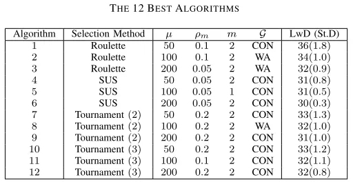
TABLE I THE12 BESTALGORITHMS
Algorithm Selection Method µ ρm m G LwD (St.D)
1 Roulette 50 0.1 2 CON 36(1.8)
2 Roulette 100 0.1 2 WA 34(1.0)
3 Roulette 200 0.05 2 WA 32(0.9)
4 SUS 50 0.05 2 CON 31(0.8)
5 SUS 100 0.05 1 CON 31(0.5)
6 SUS 200 0.05 2 CON 30(0.3)
7 Tournament(2) 50 0.2 2 CON 33(1.3)
8 Tournament(2) 100 0.2 2 WA 32(1.0)
9 Tournament(2) 200 0.2 2 CON 31(1.0)
10 Tournament(3) 50 0.2 2 CON 33(1.2)
11 Tournament(3) 100 0.1 2 CON 32(1.1)
12 Tournament(3) 200 0.2 2 CON 32(0.8) best parameters from section IV for a given selection scheme and population size. The LwD from peak power is related to the fitness function in (14) by LwD= 100−F(aν), thus the
LwD values are measured as a %.
The most effective optimisation for this scenario came from applying algorithm 6, as it found the LwD of power and with the lowest standard deviation, implying a high degree of repeatability giving us confidence in its ability to constantly return the best solution. Applying the source scaling factors provided by algorithm 6, as in figures 3(b), 3(d), and 3(f), the received power now deviated 32% between 17µW and
25µW. This improvement in power distribution also led to a change in bandwidth and rms delay spread distribution. The bandwidth now varied between 14MHz to 110MHz, which, while it showed a 24MHz reduction in the peak bandwidth, our worst case performance criteria, the lowest bandwidth remained the same. The rms delay spread ranged from 0.5ns
to1.4ns, little changed from the baseline case.
In terms of how each selection routine performed relative to each other, figure 4 shows the convergence curves of the best individual within the population for algorithms 2,6and11of table I at each generation. The curves shown are typical for a given selection scheme, with only the point of convergence changing by varying the parameters such as mutation rate, number of crossover points and genotype structure. The insert to figure 4 details the normalised ratios found in the final generation of algorithm 6 in their respective positions upon the ceiling. These ratios can be used to produce the results of figures 3(b), 3(d), and 3(f). An interesting result of these ratios and their positions is the apparent symmetry of the ratios, around the center of the ceiling. Whereas the work described in this paper, relies on fixed spot position and varying intensities, other work has been presented [40], [41], that varies spot position at fixed intensities. The elegance of applying the GA does not rule out reproducing, albeit not perfectly due to spacing of our uniform spot distribution, any of these established spot patterns, such as uniform, diamond or line-strip [15], by simply setting some of the ratios to be 0
and some to1. However the GA ratios are not restricted to any spot pattern and so, as will be shown in section V-C, could prove to be more adaptable in the event of user movement, or alternative environments.
[image:8.595.48.304.109.241.2]SUS selection routines performed the most predictably and with the best overall results. The slow and gradual convergence to a solution was always achievable, even at higher mutation
Fig. 4. Convergence curves for algorithms2,6and 11. Insert depicts the
16normalised ratios for the respective spot positions provided by the last generation of algorithm6.
rates (ρm = 0.1), although best performances were always found whenρm= 0.05. They also performed better with the concertina genotypic structure (G=CON), achieving around
1−2%improvement over a routine with identical parameters and a wrap around structure(G=WA). The use of a double point cross over (m = 2) improved the standard deviation, that is, its repeatability, but seemed to have little effect on the ability to converge to better solutions. Finally the highest population size (µ = 200), appeared to be preferential in gaining lower power deviation, compared to settingµ= 100. Tournament selection, with either2or 3tournament candi-dates, tended to quickly but sub-optimally converge. As can be seen from figure 4, beyond500 generations, the selection routine will not allow for new solutions to be considered, even when using a high mutation rate (ρm = 0.2) in order to overcome the predicted50% loss of diversity encountered from thegreedynature of the selection scheme. This high level of genotypic information removal also meant that performance was very similar whenµ= 100andµ= 200for a given set of parameters, as regardless of the information formed upon initialisation, the algorithm had no time to thoroughly search the solution space. Very little dependence was shown upon the number of crossover points used, but generally produced better results using the concertina genotype structure(G=CON).
Roulette selection was by far the worst performing of all tested, showing no consistency or pattern towards either how well an algorithm would perform, or to why a performance level was achieved. Variation of one parameter resulted in contradictory behaviour for any other developed parameter relations. Figure 4 illustrates the chaotic nature of the conver-gence curve for algorithm 2, seemingly losing good genetic information from one generation to the next.
B. Source Number and FOV Variations
Continuing with the same room, we now vary the number of sources from9to25, and the receiver’s FOV between10◦and
TABLE II
EMPTYTESTROOMPOWEROPTIMISATION USINGALGORITHM6FOR VARYINGNUMBER OFSOURCES ANDRECEIVERFOV’S
No. Spots
9 16 25
FOV NOD OLD(St.D) NOD OLD (St.D) NOD OLD (St.D)
10◦
98 98(0.0) 96 96(0.0) 94 94(0.0)
15◦ 95 95(0
.0) 92 91(0.0) 92 92(0.0)
25◦
90 90(0.0) 54 54(0.2) 60 59(0.4)
35◦ 62 56(0
.2) 61 49(0.3) 66 42(1.4)
45◦ 54 36(0
.4) 46 30(0.3) 45 29(0.3)
55◦ 45 25(0
.4) 46 25(0.3) 44 23(0.4)
65◦ 44 30(0
.2) 45 29(0.4) 45 27(0.3)
75◦ 42 30(0
.2) 42 26(0.4) 42 25(0.3)
85◦ 42 30(0
.2) 42 27(0.3) 42 26(0.3) technique will add some complexity to the transmitter driver electronics, we resisted the urge to go beyond 25sources, so as still to keep the system cost effective. Table II presents the results for the optimised lowest deviation (OLD) from peak power as a %and the standard deviation of the multiple runs using algorithm 6, compared to the non optimised deviation from peak power (NOD)(%).
For a receiver with a FOVRj <35
◦, virtually no
optimi-sation can be achieved. This is down to the fact that at these small FOV’s, the receiver does not detect much power from the multiple reflections off the surfaces of the environment, as for example figures 5(a) and 5(b) which show the before and after optimisation of a receiver with a FOVRj = 15
◦ under
16spots. In contrast to this is a receiver with a slightly higher FOVRj = 35
◦ under25spots, which is the configuration that
can be optimised the most, the power being reduced from a deviation of 66%, to 42%, as in figures 5(c) and 5(d). Using a receiver with a FOVRj = 55
◦ under 25spots provides the
configuration with the lowest optimised change in power from peak at only 23%, which can be seen in 5(e) and 5(f).
As in previous results, using the GA to reduce the deviation of the received power has negligible effects on the bandwidth and RMS delay spread. As shown in figure 6, for the lower FOV’s, where no optimisation is achieved, both the optimised and non optimised, minimum bandwidth and largest rms delay spread remain the same. For higher FOV’s, the maximum rms delay spread is relatively unchanged, and the bandwidth has been reduced by around2MHz at some FOV’s.
One affirmation to make with the bandwidth results of figure 6, is that they show our performance criteria of lowest possible bandwidth at any receiver position within the room. Whilst it can be observed that the bandwidth increases slightly with increasing FOV, a concept that may seem contrary to traditional thought, these worst case results are found near the walls of the room, as can be seen in figure 3(c-d). At these positions, a receiver and ceiling diffusion spot, are8cm
[image:9.595.51.297.135.241.2]and at least 50cm from the wall, respectively. This means that at the lower FOV’s, there is no direct LOS link present, consequently all incident radiation is a result of multiple reflections, lowering the bandwidth. As the FOV increases, more LOS links are formed, and the power from the LOS links is larger, relative to the power from reflections, increasing bandwidth. Finally, at the very large FOV’s, the worst case bandwidth reduces slightly as the magnitude of power from reflections increase relative to that from the LOS links.
Fig. 5. Empty test room power optimisation using algorithm 6 for varying number of sources and receiver FOV’s. (a) Non optimised, FOVRj = 15◦,16
spots. (b) Optimised, FOVRj = 15◦,16spots. (c) Non optimised, FOVRj =
35◦
,25spots. (d) Optimised, FOVRj = 35◦,25spots. (e) Non optimised,
FOVRj = 55 ◦
,25spots. (f) Optimised, FOVRj = 55 ◦
,25spots.
C. Moving Objects
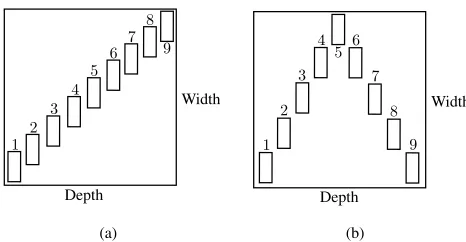
Using a simple ray tracing intersection algorithm [42], an object, representing a person with a heightz= 1.8m, shoulder to shoulder width x= 0.7m, front to back depth y = 0.4m
and reflectivity ρ = 0.3 [26], was modelled undertaking two different movement patterns as shown in figure 7. To quantify the GAs ability to work in real world scenarios, we implemented movement pattern 1 in our established en-vironment, and movement pattern 2in an environment of the same dimensions, but reducing the reflectivity of the ceiling toρ= 0.75, north wall to ρ= 0.7 and east wall toρ= 0.6. We reiterate that although the person is moving, they are not moving fast enough to break the multipath fading criteria set out in section III. Based on the results of section V-B, we implemented a system with 25 ceiling spots, with a receiver FOVRj = 55
◦, such that we are using the configuration we
thought could attain the lowest possible power deviation. Given that our receiver locations are in fixed uniformly distributed positions, and that objects are now placed within the environments, the fitness function may not correctly handle a receiverinsidean object, as the incident power will be zero. To accommodate this we place an exclusion zone, where no information is passed back to the GA, around the person of
Fig. 6. Empty test room bandwidth and rms delay spread optimisation using algorithm 6 for varying number of sources and receiver FOV’s. (a)9spots. (b)
16spots. (c)25spots.
1 2
3 4
5 6 7
8
9
Depth
Width
(a)
1 2
3 4
5 6 7
8
9
Depth
Width
[image:10.595.57.290.295.416.2](b)
Fig. 7. The nine movement positions. (a) Pattern 1. (b) Pattern 2.
This issue is a limitation of the GA, not the channel response simulation, or intersection algorithm which handled receiver’s blocked by objects correctly. We also tested algorithm 11in table I, as it uses a tournament 3 selection routine. It was shown to be capable of finding solutions to within a few%of algorithm6using a lower population size and without the need to compute proportional fitnesses, therefore allowing simpler transmitter hardware implementation, or just as importantly, exhibit a lower adaptation latency.
Considering an empty environment 1, the deviation from peak power is just under 45%, as shown in figure 8(a), and optimising using algorithm 6 and algorithm 11, reduces the deviation by around 21% and18% respectively. Environment
2 when empty, as shown in figure 8(b), has a slightly higher power deviation at 52% with algorithm 6 and algorithm 11
reducing the power deviation by 26% and24% respectively. Similar to the results of table I, algorithm 6 outperforms algorithm11by a few percent, highlighting the consistency in the GAs performance characteristics when scaled to different environments. When the person is moving in either room, they perturb the power distribution, as they themselves become reflectors, up to an influence of 19% change. We stress that this power deviation is a measure of the difference between maximum and minimum over all locations within the room, not just the receiver in use by the moving person, such that it is possible that all users are affected by the movement.
Furthermore from figure 8, both algorithms, in both envi-ronments, when exposed to different user movement patterns,
manage to track the movement, and not only maintain an optimised power distribution below the original empty room, but also now keep the effect of the moving person down to a perturbation of 12% for environment 1 and 18% for environment 2. Position 9 of environment 2 may show the first signs of the what is still a technique limited to what is physically achievable. While the algorithm has managed to reduce the deviation from peak power by 25%, it happened to be at a position in the room where the influence of the person was such that they had a very large effect on the power distribution, influencing the largest change out of all the positions in both rooms.
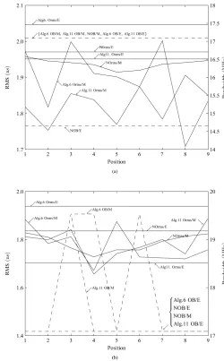
Figure 9 shows the relationship between the non-optimised bandwidth (NOB), rms delay spread (NOrms) and optimised bandwidth (OB) and rms delay spread (Orms) for both envi-ronments while empty (/E), and with movement (/M). The results reinforce further that, while the GA is capable of optimising the received power around the room, it will not alter the worst case bandwidth or rms delay spread by more
than 3 MHz, and < 0.3 ns, respectively, which may be an
acceptable compromise for the purposes of an OW system, given the advantages this technique might provide for a single optimal hardware solution to multiple dynamic environments. The final question based on these results is what FOV a designer may choose to use? For the scenarios simulated here, a receiver design would be based upon a FOVRj = 55
◦as the
GA is most effective, for our chosen metric in (14), at this FOV. However the GA method proposed, although shown to be viable and advantageous in its application, is only one stage in the design process. A specific product deployment scenario may have constraints, such as higher than average ambient light conditions, that excludes the use of a FOVRj = 55
◦.
Ideally the simulations would need to be completed in rooms encompassing the end users, their movement patterns, and the commonly found materials in the systems targeted deployment environment. The final FOV decision would then be based upon the results generated in conjunction with any ancillary considerations.
VI. CONCLUSION
Fig. 8. Power distribution in two dynamic environments. (a) Environment 1, movement pattern 1. (b) Environment 2, movement pattern 2.
the received power distribution in multiple dynamic environ-ments. Careful analysis of the GA performance has resulted in several relationships between population size, selection scheme, mutation rate and genotype structure. Two algorithms in particular have been highlighted as possible candidates for a final application solution. In an empty room algorithm
6 produced a highly repeatable improvement in the power distribution, reducing deviation by up to24%, whilst algorithm
11 produced marginally lower improvements, but benefited from being a much more practical algorithm to implement. In the mobile scenarios shown, the GA managed to reduce power deviation by up to 26%, and forming, while the user perturbed the channel, a consistent power distribution to within
12%. Furthermore, the optimisation of the power distribution was carried out with only negligible impact to bandwidth and rms delay spread. Based upon the simulation conducted, work could be carried out on producing a optimal receiver design with regards to complexity, power efficiency and cost, using a FOVRj = 55
◦ for mass product integration.
Fig. 9. Bandwidth and rms delay spread in two dynamic environments. (a) Environment 1, movement pattern 1. (b) Environment 2, movement pattern 2.
REFERENCES
[1] F. R. Gfeller and U. Bapst, “Wireless in-house data communication via diffuse infrared radiation,”Proc. IEEE, vol. 67, no. 11, pp. 1474–1486, 1979.
[2] A. J. C. Moreira, R. T. Valadas, and A. M. de Oliveira Duarte, “Optical interference produced by artificial light,”Wirel.Netw., vol. 3, no. 2, pp. 131–140, 1997.
[3] H. Hashemi, G. Yun, M. Kavehrad, F. Behbahani, and P. A. Galko, “Indoor propagation measurements at infrared frequencies for wireless local area networks applications,”IEEE Trans. Veh. Technol., vol. 43, no. 3, pp. 562–576, 1994.
[4] D. C. O’Brien, M. Katz, P. Wang, K. Kalliojarvi, S. Arnon, M. Mat-sumoto, R. J. Green, and S. Jivkova, “Short range optical wireless communications,”Wireless World Research Forum, 2005.
[5] P. Djahani and J. M. Kahn, “Analysis of infrared wireless links em-ploying multibeam transmitters and imaging diversity receivers,”IEEE Trans. Commun., vol. 48, no. 12, pp. 2077–2088, 2000.
[6] R. Ramirez-Iniguez and R. J. Green, “Optical antenna design for indoor optical wireless communication systems,”Int. J. Commun. Syst., vol. 18, no. 3, pp. 229–245, 2005.
[7] M. F. L. Abdullah, “Techniques for signal to noise ratio adaptation in infrared optical wireless for optimisation of receiver performance,” Ph.D. dissertation, 2007.
[image:11.595.307.557.110.513.2]pulse-position modulation for indoor wireless infrared communications,”IEEE Trans. Commun., vol. 45, no. 9, pp. 1080–1087, 1997.
[9] H. Uno, K. Kumatani, H. Okuhata, I. Shirakawa, and T. Chiba, “ASK digital demodulation scheme for noise immune infrared data communi-cation,”Wirel.Netw., vol. 3, no. 2, pp. 121–129, 1997.
[10] R. J. Dickenson and Z. Ghassemlooy, “A feature extraction and pattern recognition receiver employing wavelet analysis and artificial intelli-gence for signal detection in diffuse optical wireless communications,”
IEEE Trans. Wireless Commun., vol. 10, no. 2, pp. 64–72, 2003. [11] S. Kirkpatrick, C. D. Gelatt, and M. P. Vecchi, “Optimization by
simulated annealing,”Science, vol. 220, no. 4598, pp. 671–680, 1983. [12] D. W. K. Wong, G. Chen, and J. Yao, “Optimization of spot pattern
in indoor diffuse optical wireless local area networks,”Opt. Express, vol. 13, no. 8, pp. 3000–3014, 2005.
[13] M. Wen, J. Yao, D. W. K. Wong, and G. C. K. Chen, “Holographic diffuser design using a modified genetic algorithm,”Opt.Eng., vol. 44, no. 8, pp. 085 801–8, 2005.
[14] P. L. Eardley, D. R. Wisely, D. Wood, and P. McKee, “Holograms for optical wireless lans,”IEE Proc. Optoelectron., vol. 143, no. 6, pp. 365– 369, 1996.
[15] A. G. Al-Ghamdi and J. M. H. Elmirghani, “Analysis of diffuse optical wireless channels employing spot-diffusing techniques, diversity receivers, and combining schemes,” IEEE Trans. Commun., vol. 52, no. 10, pp. 1622–1631, 2004.
[16] H. Yang and C. Lu, “Infrared wireless lan using multiple optical sources,”IEE Proc. Optoelectron., vol. 147, no. 4, pp. 301–307, 2000. [17] V. Pohl, V. Jungnickel, and C. von Helmolt, “Integrating-sphere diffuser for wireless infrared communication,”IEE Proc. Optoelectron., vol. 147, no. 4, pp. 281–285, 2000.
[18] T. Komine and M. Nakagawa, “Fundamental analysis for visible-light communication system using led lights,”IEEE Trans. Consum. Electron., vol. 50, no. 1, pp. 100–107, 2004.
[19] S. Jivkova, B. A. Hristov, and M. Kavehrad, “Power-efficient multispot-diffuse multiple-input-multiple-output approach to broad-band optical wireless communications,”IEEE Trans. Veh. Technol., vol. 53, no. 3, pp. 882–889, 2004.
[20] D. C. O’Brien, G. E. Faulkner, E. B. Zyambo, K. Jim, D. J. Edwards, P. Stavrinou, G. Parry, J. Bellon, M. J. Sibley, V. A. Lalithambika, V. M. Joyner, R. J. Samsudin, D. M. Holburn, and R. J. Mears, “Integrated transceivers for optical wireless communications,”IEEE J. Sel. Topics. Quantum Electron., vol. 11, no. 1, pp. 173–183, 2005.
[21] C. R. Lomba, R. T. Valadas, and A. M. O. Duarte, “Experimental characterisation and modelling of the reflection of infrared signals on indoor surfaces,”IEE Proc. Optoelectron., vol. 145, pp. 191–197, 1998. [22] B. T. Phong, “Illumination for computer generated pictures,”Commun
ACM, vol. 18, no. 6, pp. 311–317, 1975.
[23] S. R. Perez, R. P. Jimenez, F. J. L. Hernandez, O. B. G. Hernandez, and A. J. A. Alfonso, “Reflection model for calculation of the impulse response on ir-wireless indoor channels using ray-tracing algorithm,”
Microwave. Opt. Technol. Lett., vol. 32, no. 4, pp. 296–300, 2002. [24] J. M. Kahn, W. J. Krause, and J. B. Carruthers, “Experimental
characteri-zation of non-directed indoor infrared channels,”IEEE Trans. Commun., vol. 43, no. 234, pp. 1613–1623, 1995.
[25] J. R. Barry, J. M. Kahn, W. J. Krause, E. A. Lee, and D. G. Messer-schmitt, “Simulation of multipath impulse response for indoor wireless optical channels,”IEEE J. Sel. Areas Commun., vol. 11, no. 3, pp. 367– 379, 1993.
[26] J. B. Carruthers, S. M. Carroll, and P. Kannan, “Propagation modelling for indoor optical wireless communications using fast multi-receiver channel estimation,”IEE Proc., Optoelectron., vol. 150, no. 5, pp. 473– 481, 2003.
[27] J. B. Carruthers and P. Kannan, “Iterative site-based modeling for wireless infrared channels,” IEEE Trans. Antennas Propag., vol. 50, no. 5, pp. 759–765, 2002.
[28] J. B. Carruthers and J. M. Kahn, “Modeling of nondirected wireless infrared channels,”IEEE Trans. Commun., vol. 45, no. 10, pp. 1260– 1268, 1997.
[29] BS EN 60825-1:1994: Safety of laser products. Equipment classification, requirements and user’s guide, Std.
[30] A. C. Boucouvalas, “IEC 825-1 eye safety classification of some consumer electronic products,”IEE Seminar Digests, vol. 1996, no. 32, pp. 13/1–13/6, 1996.
[31] I. Haratcherev, J. Taal, K. Langendoen, R. Lagendijk, and H. Sips, “Automatic ieee 802.11 rate control for streaming applications,”Wireless Commun. Mob. Comput., vol. 5, no. 4, pp. 421–437, 2005.
[32] A. Garcia-Zambrana and A. Puerta-Notario, “Novel approach for in-creasing the peak-to-average optical power ratio in rate-adaptive optical wireless communication systems,”IEE Proc., Optoelectron., vol. 150, no. 5, pp. 439–444, 2003.
[33] M. R. Pakravan and M. Kavehrad, “Indoor wireless infrared channel characterization by measurements,”IEEE Trans. Veh. Technol., vol. 50, pp. 1053–1073, 2001.
[34] T. B¨ack, U. Hammel, and H. P. Schwefel, “Evolutionary computation: Comments on the history and current state,”IEEE Trans. Evol. Comput., vol. 1, no. 1, pp. 3–17, 1997.
[35] F. Rothlauf, Representations for genetic and evolutionary algorithms. Physica-Verlag, 2002.
[36] F. O’Karray and C. W. D. Silva,Soft computing and intelligent systems design : theory, tools, and applications. Pearson/Addison Wesley, 2004. [37] T. B¨ack, Evolutionary algorithms in theory and practice : evolution strategies, evolutionary programming, genetic algorithms. Oxford University Press, 1996.
[38] J. E. Baker, “Reducing bias and inefficiency in the selection algorithm,” inProc. 2nd Int. Conf. Genetic Algorithms and their application, 1987. [39] R. Poli, “Tournament selection, iterated coupon-collection problem, and backward-chaining evolutionary algorithms,” inFoundations of Genetic Algorithms, 2005, pp. 132–155.
[40] A. G. Al-Ghamdi and J. M. H. Elmirghani, “Analysis of optical wireless links employing a beam clustering method and diversity receivers,” in
IEEE Int. Conf. Commun., vol. 6, 2004, pp. 3341–3347.
[41] G. Yun and M. Kavehrad, “Spot-diffusing and fly-eye receivers for indoor infrared wireless communications,” inIEEE Int. Conf. Sel. Topics Wireless Commun., 1992, pp. 262–265.
[42] A. S. Glassner, “Space subdivision for fast ray tracing,”IEEE Comput. Graph. Appl., vol. 4, no. 10, pp. 15–22, 1984.
Matthew D. Higginsreceived his MEng degree in Electronic and Commu-nications Engineering in 2005 from the University of Warwick, UK, and is currently working towards his PhD at the same institution. His major area of research is focused on mobile optical wireless communications systems, specifically the use of genetic algorithms for channel optimisation, and the application of nonlinear devices for receiver technology. Matthew is a Member of the IET and Student Member of both the IEEE and SPIE.
Roger J. Green became Professor of Electronic Communication Systems at Warwick in September 1999, and Head of the Division of Electrical and Electronic Engineering in August 2003. He has published over 190 papers in the field of optical communications, optoelectronics, video and imaging, and has several patents. Some 46 PhD research students have worked successfully under his supervision. He leads the Communications and Signal Processing Research Group, which is the largest in the School of Engineering at Warwick. His current interests include optical detection systems in communications and imaging technology. He is a Fellow of the IET and has served on IEE committee E14. He is also a Senior Member of the IEEE, and currently serves on two IEEE committees concerned with communications and signal processing. He has been a member of the EPSRC College since 2002, and is a member of the Engineering Professors’ Council. He has formed two Warwick spin-offs - Shibden Limited and Optical Antenna Solutions.
![Fig. 1.Source, receiver and reflector geometry, adapted from [25]](https://thumb-us.123doks.com/thumbv2/123dok_us/9717471.472726/4.595.60.287.112.304/fig-source-receiver-reector-geometry-adapted.webp)