The Inter-related Dynamics of Unemployment and Low-Wage
Employment
Mark Stewart
No 741
WARWICK ECONOMIC RESEARCH PAPERS
The Inter-related Dynamics of
Unemployment and Low-wage
Employment
Mark B. Stewart
∗University of Warwick
December 2005
Abstract
This paper examines the extent of state dependence in unemployment and the role played in this by intervening low-wage employment. A range of dy-namic random and fixed effects estimators are compared. Low-wage employ-ment is found to have almost as large an adverse effect as unemployment on future prospects and the difference in their effects is found to be insignificant. Evidence is presented that low-wage jobs act as the main conduit for repeat unemployment and considerably increases its probability. Obtaining a higher-wage job reduces the increased risk of repeat unemployment to insignificance.
JEL classification: J64, J31, C25, C23.
Key words: unemployment dynamics, low-wage employment, state dependence, unobserved heterogeneity, dynamic random effects models, repeat unemployment.
∗Address for correspondence: Mark Stewart, Economics Department, University of Warwick, Coventry CV4 7AL, UK. Tel: (44/0)-24-7653-3043. Fax: (44/0)-24-7652-3032.
1
Introduction
Repeat unemployment is common: a significant proportion of the unemployed who
get re—employed leave their jobs again relatively quickly.1 As Heckman (2001)
ob-serves in his Nobel lecture, “a frequently noted empirical regularity in the analysis of
unemployment data is that those who were unemployed in the past or have worked
in the past are more likely to be unemployed (or working) in the future” (p. 706).
Is this, he asks, “due to a causal effect of being unemployed (or working) or is it
a manifestation of a stable trait?” There is also strong persistence in wages, and
these dynamics are also linked. Those in low-wage jobs are more likely to become
unemployed, and the unemployed are more likely to be low waged on re-entry to
employment. This paper investigates these inter-related dynamics of unemployment
and low-wage employment.
Several previous studies have investigated the extent of state dependence in
em-ployment or unemem-ployment.2 Heckman (1981a) found significant state dependence in
the employment probabilities of older US married women (but rather less for younger
women). More recently Hyslop (1999) alsofinds strong state dependence in
employ-ment for US married women for the 1980s. Corcoran and Hill (1985) however find
that past unemployment does not increase the probability of current unemployment
for prime age men once unobserved heterogeneity and data collection procedures have
been allowed for.3 For Britain, Narendranathan and Elias (1993) and Arulampalam
et al. (2000) find strong state dependence in unemployment.4 Similar has also been
1Clark and Summers (1979) for the US and Layard et al. (1991) for the UK inter alia. About
half of those leaving the unemployed claimant count in Britain return within a year (Sweeney, 1996).
2While evidence on each is clearly indicative about the other, they are not equivalent. Flinn and
Heckman (1983)find unemployment and out of the labour force to be behaviourally distinct states in the context of transitions.
3Analyses of durations include Heckman and Borjas (1980) and Lynch (1989), who find no
ev-idence that previous occurrences or durations of unemployment affect the duration of current un-employment spells of US youths, and Omori (1997), who in contrastfinds that an increase in the duration of previous non-employment lengthens the duration of current non-employment.
4For dependence between durations however, Lynch (1985)finds the length of previous
found for Germany (Flaig et al., 1993, Muhleisen and Zimmermann, 1994) and
Hol-land (Frijters et al., 2000) among other countries.
Much of the evidence indicates that experiencing unemployment makes future
unemployment more likely. However we know little about the mechanism that lies
behind this state dependence. The evidence presented in this paper suggests that
an important part of the reason is the quality of the jobs taken by those who move
into employment, which tend to be low paid and unstable. Thus a fuller picture of
the dynamics of unemployment is provided by examining it in conjunction with the
type of job taken when an exit from unemployment occurs. There is also evidence of
persistence in low pay,5 and of a link between them giving a cycle of unemployment
and low-wage employment (Stewart, 1999).6
State dependence in unemployment is generally viewed as resulting from the non—
accumulation of new (and the deterioration of existing) human capital during an
unemployment spell and from adverse signalling. Low-wage jobs may also not
aug-ment human capital and hence have similar adverse effects to unemployment. The
distinction between low- and higher-wage jobs is one dimension of the “good” and
“bad” jobs distinction (Burtless et al., 1990, Acemoglu, 2001). Layard et al. (1990)
argue that “employers offering good jobs may well use a person’s current position as
a screening device. While unemployment is a bad signal, being in a low—quality job
may well be a worse one” (p. 249).7 McCormick (1990) terms such jobs “stigmatized”
and argues that, faced by uncertainty about worker quality,firms use type of job held,
alongside unemployment duration (Blanchard and Diamond, 1994), as a cheap
indica-tor of future productivity. This paper examines the extent to which “bad” jobs have
adverse effects on future employment prospects, alongside those of unemployment,
5See Stewart and Swaffield (1999). There is also an extensive literature on wage persistence
and wage dynamics in general, not focusing specifically on the bottom end of the distribution. See Moffitt and Gottschalk (1993), Baker (1997) and Dickens (2000) for recent contributions.
6There is considerable US evidence of significant long-lasting earnings losses associated with job
displacement (e.g. Jacobson et al., 1993, Kletzer, 1998). Gregg and Wadsworth (2000) and Gregory and Jukes (2001)find a negative impact of unemployment on subsequent earnings for Britain.
7Such effects may also result from efficiency wage, insider outsider, or segmented labour market
and the extent to which they act as the conduit to repeat unemployment.8
This paper uses a discrete time framework to analyze the inter-related dynamics
of unemployment and low-wage employment. While a continuous time multi-spell
duration model might be a preferable framework to analyze unemployment alone,
since the central focus here is the relationship with (low) wages, and since the dataset
used (in common with others) provides wage information only at the interview point
for each annual wave of the panel, a discrete time framework is adopted.
The central econometric issue in the dynamic models used is that of unobserved
heterogeneity and initial conditions. The paper addresses this in a number of ways
and presents and compares the estimates from a number of alternative estimators to
assess the robustness of the results. A range of dynamic random effects probit model
estimators is used. Both normal heterogeneity and a semi-parametric discrete
mix-ture are used. Models with autocorrelated errors, with bivariate random effects and
with random effects on slope as well as intercept, estimated by Maximum Simulated
Likelihood, are also considered. The dynamic random effects probit model estimators
are also compared with various GMM estimators in the context of a linear probability
model, which handle unobserved heterogeneity in a less restrictive way.
The estimates show strong agreement between the estimators used. Significant
state dependence in unemployment is found. Low-wage employment is found to have
almost as large an adverse effect as unemployment on the probability of future
unem-ployment, and the effects are insignificantly different from one another. In addition,
low-wage jobs are found to act as the main conduit for repeat unemployment, those
who get a better job reduce the impact of past unemployment to insignificance.
8The link between low-wage employment and unemployment may also be related to
2
Data description
The data used in the paper are from the first six waves (1991—1996) of the British
Household Panel Survey (BHPS).9 The BHPS contains a nationally representative
sample of households whose members are re-interviewed each year.10 The sample
used in this paper is restricted to those who were in the labour force (employed or
unemployed) at the time of interview. The starting sample contains 23,491
observa-tions on 4,739 individuals and forms an unbalanced panel. 3,060 of these individuals
are observed in the labour force in all 6 waves.
The unemployment indicator used is constructed on the basis of the ILO/OECD
definition of unemployment. Under this definition a person is unemployed if he or she
does not have a job, but had looked for work in the past four weeks and is available
for work. The probabilities of unemployment (both unconditional and conditional
on status at t—1) over waves 2—6 (1992—1996) of the sample for various groups are
presented in Table 1. The raw unconditional probability of being unemployed at a
point in time in this sample is 4.4%.11 Columns 2 and 3 of the table give conditional
probabilities by status att—1, i.e. at the previous interview roughly 12 months
previ-ously.12 The first row of the table shows that there is considerable state dependence
in unemployment in the raw data: the probability of being unemployed at t is much
higher for those unemployed at t—1. Someone unemployed at t—1 is more than 20
times as likely to be unemployed att as someone employed at t—1.
Part, or even all, of the persistence exhibited in thefirst row of Table 1 could be due
to heterogeneity. The probability of unemployment is higher for the young, for those
with less education, for those with poor health, etc. Even if there were no structural
9All time points are therefore prior to the introduction of the UK national minimum wage. 10See Taylor (1996) for details. The sample used here contains only Original Sample Members,
is restricted to those aged between 18 and the state retirement age (65 for men and 60 for women) and excludes full-time students.
11Conditional on being in the labour force (i.e. either employed or unemployed) att, but
uncon-ditional on status att—1.
1272% of the pooled sample are interviewed within 30 days of the anniversary of the previous
persistence for individuals, this heterogeneity would cause the group of individuals
unemployed att—1 to have a higher aggregate probability of unemployment att than
those who were employed.
The remaining rows of Table 1 present unemployment probabilities (unconditional
and conditional) for various subgroups of the sample distinguished by gender,
educa-tion, experience, marital status, health, area of residence, and demand conditions in
the local labour market (factors likely to influence the probability of unemployment
and suitable variables for the models later in the paper.) The difference between the
probabilities conditional on status att—1 is evident within all subgroups.
The data also exhibits considerable persistence in wages and the aggregate
dy-namic processes are inter-related: the current probability of each depends on the past
occurrence of the other. The role of low-wage employment is a focus of this paper.
If those employed at t—1 (column 2 of Table 1) are partitioned into those with a
low wage (below £3.50 per hour in 1997 terms13) and those with a higher wage, the
conditional probability of being unemployed att is 0.056 for the low-wage group and
0.020 for the higher-wage group. Employees with a low-wage att—1 are 2.7 times as
likely to be unemployed at t as those who were higher paid at t—1. Compared with
the pairs of rows in column 2, a low wage at t—1 has a considerably more adverse
effect on the probability of unemployment att than the characteristics considered in
Table 1. Those unemployed at t—1 are also nearly three times as likely to be low
wage if employed attas those employed att—1. There is therefore considerable
cross-persistence in the aggregate data. Table 2 summarizes the definitions of these two
variables and also those for the main explanatory variables used in the analysis and
presents summary statistics (means and standard deviations) for these variables.
3
Models and estimators
This paper uses a range of dynamic models and estimators to model the probability of
unemployment, both singly and jointly with the probability of low-wage employment.
The models include the previous state to allow for state dependence. An important
focus is the treatment of unobserved heterogeneity and initial conditions. If the
unobserved heterogeneity exhibits persistence over time, then ignoring it will lead to
an overstatement of the true state dependence in unemployment.
3.1
A dynamic random e
ff
ects probit model
The following dynamic reduced form model for unemployment is specified:
yit=1(x0itβ+γyit−1 +εi+uit >0) (i= 1, . . . , N;t = 2, . . . , T) (1)
whereyit is the indicator variable for being unemployed,xitis a vector of explanatory
variables anduit ∼N(0, σ2u). The subscripti indexes individuals andt time periods.
N is large, but T is small and fixed, so asymptotics are on N alone. Although the
uit are assumed iid, the composite error term will be correlated over time due to the
individual—specific time—invariantεi terms. The standard uncorrelated random effects
model also assumesεi uncorrelated withxit. Alternatively, following Mundlak (1978)
and Chamberlain (1984), correlation between εi and the observed characteristics is
allowed by assuming a relationship of the form: εi =x0ia+αi, whereαi ∼iidN(0, σ2α)
and independent ofxit anduit for alli, t. Thus the model may be written as:
yit =1(x0itβ+γyit−1+x0ia+αi+uit >0) (i= 1, . . . , N;t= 2, . . . , T) (2)
The individual-specific random effects specification adopted implies that the
cor-relation between vit = αi +uit in any two (different) periods will be the same:
λ = Corr(vit, vis) = σ2α/(σα2 +σ2u) for t, s = 2, . . . , T;t 6= s. Estimation requires
an assumption about the relationship between the initial observations,yi1, andαi. If
the initial conditions are taken to be exogenous, appropriate if the start of the process
decomposes and a standard random effects probit program can be used. If the initial
conditions are correlated with the αi, as would be expected in the current context,
this method of estimation overstates state dependence (e.g. Chay and Hyslop, 2000).
3.2
Heckman’s estimator
The approach to the initial conditions problem proposed by Heckman (1981b) involves
specifying a linearized reduced form equation for the initial period:
yi1 =1(zi01π+ζi >0) (3)
where zi1 includes xi1 and exogenous instruments and ζi is correlated with αi, but
uncorrelated withuit fort ≥2. Using an orthogonal projection, it can be written as:
ζi =θαi+ui1, with αi and ui1 independent of one another. It is also assumed that
ui1 satisfies the same distributional assumptions as uit for t ≥ 2.14 The linearized
reduced form for the initial period is therefore specified as
yi1 =1(zi01π+θαi+ui1 >0) (4)
Since y is binary, a normalization is required. A convenient one is σ2
u = 1. The
outcome probabilities and likelihood for a random sample are then
Pit(α∗) =
½ Φ[(x0
itβ+γyit−1+x0ia+σαα∗)(2yit−1)] for t ≥2
Φ[(z0
i1π+θσαα∗)(2yi1−1)] for t = 1
(5)
L=
N
Y
i=1
Z
α∗
( T
Y
t=2
Pit(α∗)
)
dF(α∗) (6)
where F is the distribution function of α∗ = α/σ
α and σα =
p
λ/(1−λ). If α
is taken to be normally distributed, the integral over α∗ can be evaluated using
Gaussian—Hermite quadrature (Butler and Moffitt, 1982).
3.3
Wooldridge’s CML estimator
The Heckman estimator approximates the joint probability of the full observedy
se-quence. Wooldridge (2005) has proposed an alternative Conditional Maximum
Likeli-hood (CML) estimator that considers the distribution conditional on the initial period
value (and exogenous variables). Rather than modelling the density of (yi1, . . . , yiT)
given xi, Wooldridge suggests modelling the density of (yi2, . . . , yiT) conditional on
(yi1, xi). This produces a very simple estimation method which has the advantage
that it can be implemented with standard random effects probit software.15
The estimator can be viewed as simply using a different approximation which has
computational advantages. Specifying a model for yi1 given xi andαi is replaced by
specifying one forαi givenyi1andxi. The model forαiis specified in its simplest form
asαi =a0 +a1yi1+ξi. (The Mundlak specification above has already incorporated
xi.) Substituting into equation (2) gives
yit=1(x0itβ+γyit−1+a0+a1yi1+x0ia+ξi+uit >0) (7)
The estimates presented here also follow Wooldridge’s suggestion of allowing a more
flexible conditional mean by including interactions betweenyi1 andxi.
3.4
A discrete distribution for the unobserved heterogeneity
Both the Heckman and Wooldridge estimators are potentially sensitive to the
nor-mality assumption on the individual effects. An alternative specification, useful
for assessing this sensitivity, is to model the unobserved heterogeneity using a
dis-crete mass point distribution. In this specification the distribution of αi is taken to
have mass points α(j) (j = 1, . . . , J) with corresponding probabilities wj satisfying
0≤wj ≤1 ∀j andPJj=1wj = 1. The outcome probabilities and likelihood are
Pit(α) =
½
Φ[(x0itβ+γyit−1+x0ia+α)(2yit−1)] for t ≥2
Φ[(z0
i1π+θα)(2yi1−1)] fort = 1 (8)
L=
N
Y
i=1
( J
X
j=1
wj
" T Y
t=1
Pit(α(j))
#)
(9)
3.5
Autocorrelated errors
Autocorrelation in the uit, perhaps reflecting correlation between transitory shocks,
complicates estimation considerably. Extension of the Heckman estimator to this case
15For example, xtprobit in Stata. This is in contrast to the Heckman estimator described above and
requires the evaluation of T-dimensional integrals of Normal densities. Simulation
estimators provide a feasible way to address this problem. A Maximum Simulated
Likelihood (MSL) estimator based on the GHK algorithm (see for example Keane,
1994) is used in this paper. MSL provides a consistent estimator of the parameters as
the number of simulation draws tends to infinity. In practice Monte Carlo evidence
suggests that a relatively small number of draws is sufficient (e.g. Hyslop (1999),
App. 2). Train (2003) shows that the number of draws required can be further reduced
(by a factor of 10 or more) by using Halton sequences. These provide better coverage
than standard random draws and negative correlation results in variance reduction.
There is now considerable evidence for their greater efficiency (Train, 2003).
The model is as above but withuit following an AR(1) process, with parameterρ.
Ω, the covariance matrix of vi = (vi1, . . . , viT)0 is now a function of λ, θ and ρ. The
error vector can be written vi = Cηi with ηi ∼ N(0, I) and C the lower-triangular
Cholesky decomposition ofΩ. The equations can therefore be written
yit =1(μit+ t
X
j=1
ctjηij >0) (10)
where μit = x0itβ +γyit−1 +xi0a for t ≥ 2 and μi1 = zi01π. The GHK algorithm
uses the fact that the probability of an observed sequence of ys can then be written
as the product of recursively defined conditional probabilities. Simulation of the
probabilities requires draws from a truncated Normal. Ifξitis a draw from a standard
uniform distribution, then these are constructed as Φ−1[(1−ξit)Φ(Lit) +ξitΦ(Uit)],
where (Lit, Uit) = (−ait,∞) if yit = 1 or (−∞,−ait) if yit = 0. The steps in the
GHK simulator for this model are therefore: (1) Calculate ai1 = μi1/c11. (2) Draw
ξi1 from a standard uniform and calculate ηr
i1 = Φ−1[(1− ξ
r
i1)Φ(Li1) + ξri1Φ(Ui1)]
and ar
i2 = (μi2 +c21ηir1)/c22. (3) Draw ξri2 from a standard uniform and calculate
ηri2 =Φ−1[(1−ξ r
i2)Φ(Lri2) +ξ r
i2Φ(Uir2)]andari3 = (μi3+c31ηri1+c32ηri2)/c33. Repeat this
step successively for the remaining time periods. The simulated likelihood is given by
L∗ =
N Y i=1 ( 1 R R X r=1 "
Φ((2yi1−1)ai1) T
Y
t=2
Φ((2yit−1)arit)
#)
3.6
Bivariate random e
ff
ects models
The model of Section 3.1 can be extended to allow correlated random effects on two
endogenous variables (e.g. unemployment and low-wage employment). The model
used here is a modified version of that used by Alessie et al. (2005). Let y1it = 1 if
individuali is unemployed at t and = 0 if employed. Lety2it = 1 if i is in low-wage
employment att and= 0 otherwise. The model for t= 2, . . . , T is specified as
y1it = 1(x01itβ1+γ11y1it−1+γ12y2it−1+α1i+u1it >0) (12)
y2it = 1(x02itβ2+γ21y1it−1+γ22y2it−1+α2i+u2it >0)if y1it = 0 (13)
The time-means,xi, have been subsumed into thex-vectors to simplify notation. The
errors (u1, u2) are assumed independent over time and jointly normally distributed
with unit variances and correlation ρu. The random effects (α1, α2) are assumed
jointly normally distributed with variancesσ2
1 andσ22 and correlation ρα.
If γ12 = 0, equation (12) can be considered on its own and (β1, γ11, σ1)
esti-mated consistently by the Heckman estimator. If γ12 6= 0, but ρu = ρα = 0, then
y2it−1 is weakly exogenous in (12), which can again be considered on its own and
(β1, γ11, γ12, σ1)estimated consistently by the Heckman estimator withy2it−1included
as a (weakly exogenous) regressor. In the cross-correlated case the bivariate model of
this section is required.
The likelihood function is given by
L=
N
Y
i=1
Z
α2 Z
α1
Pi(α1, α2)fi(α1, α2)dα1dα2 (14)
wheref is the joint density (bivariate normal) of(α1, α2)andPiis the joint probability
of the observed binary sequence for individuali(as a function of the random effects):
Pi(α1, α2) = T
Y
t=1
{y1itΦ(μ1it) + (1−y1it)Φ2(−μ1it, q2itμ2it;−q2itρu)} (15)
whereq2it = (2y2it−1), Φ2 is the cumulative bivariate normal distribution function,
μjit=x0
form approximation for period 1 as in Section 3.2. The model is estimated by MSL.
Modified versions of this bivariate random effects model are also used to (i) address the
distinction between quits and layoffs, and (ii) distinguish between continuing spells
of unemployment and repeat or new unemployment spells. Both these applications
require only minor definitional modifications to the model described above.
3.7
Heterogeneity in state dependence
A different bivariate random effects model that allows heterogeneity in a slope
coef-ficient is also used. The model in Section 3.1 assumes a constant state dependence
parameter, γ. A potentially useful generalization allows heterogeneity in this effect,
possibly correlated with the heterogeneity in the intercept. This model is specified as
yit =1(x0itβ+ (γ+α2i)yit−1+α1i+uit>0) (16)
The model is estimated by MSL, with simulator as for the previous model and
prob-abilities of observed sequences given by
Pi(α1, α2) = T
Y
t=1
{yitΦ(μit) + (1−yit)Φ(−μit)} (17)
where μit = x0
itβ + (γ + α2i)yit−1 + x0ia +α1i for t ≥ 2 and with an equivalent
approximation to the reduced form for thefirst period.
3.8
GMM estimation of a DLP model
The dynamic random effects probit models in the previous subsections require an
auxiliary distributional assumption on the individual-specific effects. This subsection
considers a GMM estimator, in the context of a dynamic linear probability (DLP)
model, not requiring such an assumption. It can be viewed as semi-parametric, being
non-parametric for the individual-specific effects. The model is specified as:
yit =x0itδ1+δ2yit−1+fi+gt+ωit (t= 2, . . . , T and i= 1, . . . , N) (18)
Differencing removes the individual-specific effects:
Even if theωit are serially independent,∆yit−1 and∆ωit will be correlated and OLS
applied to this differenced equation biased and inconsistent. A range of Instrumental
Variable estimators have been proposed to provide consistent estimation. The now
commonly used Arellano and Bond (1991) GMM estimator, involving a different
number of instruments in each time period, is based on the moment conditions
E(yit−s∆ωit) = 0, fort = 3, . . . , T ands≥2. (20)
This gives(T −1)(T −2)/2 orthogonality conditions (= 10 in the current context).
This estimator provides efficiency gains over the simpler IV estimators proposed by
Anderson and Hsiao (1981), which use for example yit−2 or ∆yit−2 to instrument
∆yit−1. The results for these estimators are examined for comparison below. The
consistency of all these estimators requires the ωit to be serially uncorrelated. The
Arellano and Bond (1991) test on the second order residual correlation coefficient is
used below, along with a Sargan test of the over-identifying restrictions.
For situations whereT is small andδ2 large Blundell and Bond (1998) propose a
“system” GMM estimator based on stacking equations infirst differences and
equa-tions in levels, with The Arellano-Bond instruments used for the first-differenced
equations and∆yi2, . . . ,∆yiT−1 used as instruments for the levels equations. System
GMM estimates are also examined below for robustness.
4
Empirical results
4.1
Random e
ff
ects probit estimates
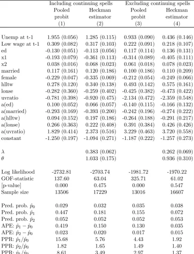
Estimates of the dynamic random effects probit model for the probability of being
unemployed using the Heckman estimator are given in Column 2 of Table 3. The
x-vector contains the variables listed in Table 2 plus year dummies. The model also
contains means over time for each time-varying variable (as specified in Section 3.1).
The corresponding pooled probit model (without random effects) estimated on the
pre-first-wave variables related to labour market entry are used as instruments.16 In
the estimated linearized reduced form for the initial condition this set of instruments
(i.e. the variables in z excluding the period 1 values of the x variables) are jointly
highly significant.17 Indicators for unemployment and low wage at t—1 are included,
with those with a higher wage being the base group. In the context of the bivariate
framework of Section 3.6 these estimates assume independence.
The dynamic random effects probit model and the pooled probit model involve
different normalizations.18 For comparisons the former needs to be multiplied by an
estimate ofσu/σv =
√
1−λ. The scaled coefficient estimate on unemployment att—1
in Column 2 is 1.01. Compared with the pooled probit estimate, the estimate ofγ is
reduced by almost half in the random effects model, but remains strongly significant.
Those who are unemployed at t—1 and again at t consist of two rather different
groups. First there are those for whom the two points in time are part of a continuing
spell without employment. Second there are those who have an intervening spell of
employment (or possibly more than one), but then are unemployed again att. This
second category is what might be labelledrepeat unemployment. The implications of
continuing spells and repeat unemployment are very different.19
This distinction can be considered in the framework of the bivariate model of
Sec-tion 3.6. The three categories are employment, continuing unemployment, and repeat
unemployment. The model is given by equations (12) and (13), but with dependent
variables defined as y1i = 1 if individual i is unemployed in a continuing spell, and
16Specifically dummy variables for father’s broad SEG at the time the respondent was 14 (together
with dummies for father not working and father deceased), similar variables in relation to the respondent’s mother at the same date, an indicator for whether or not thefirst labour market spell after leaving full-time education was an employment spell, dummy variables for the broad SEG of the first job held (after leaving full-time education), an indicator of whether this first job was a temporary job, and an indicator of whether the individual left thisfirst job due to redundancy.
17A χ2(13)Wald test statistic of 91.8, giving a p-value <0.0001.
18See Arulampalam (1999). The random effects probit estimates are normalized onσ2
u= 1, while
the pooled probit estimates are normalized on σ2
v = 1. Thus random effects probit estimation
provides an estimate ofγ/σu, while pooled probit estimation provides an estimate ofγ/σv.
19Ellwood (1982) analysed the problem caused by continuing spells when the observation period
y2i = 1 if individual i is unemployed in a new spell. In the case of independence,
the equation fory2 can be estimated on its own on the sample excluding continuing
spells, the selection involved is exogenous, and the Heckman estimator of Section 3.2
can be used. The results are given in the fourth column of Table 3. The pooled probit
estimates are given in column 3 for comparison. For comparability with the
corre-sponding models in the first two columns they are under the restriction γ21 = γ22.
Excluding continuing spells cuts the scaled estimate of the coefficient on lagged
unem-ployment by over two-thirds and that on lagged low wage by over one-third, although
both remain significantly greater than zero.20
A bivariate model without independence imposed was also estimated (by MSL)
to address the possible endogenous selection of excluding continuing spells from the
estimates in column 4 of the table.21 The coefficients on lagged unemployment and
lagged low wage are similar to those in column 4 of Table 3 and the model does not
reject independence.
There are a number of ways in which the partial, or marginal, effect of yit−1 on
P(yit = 1) can be estimated for models and estimators of this type. The method
used here is based on estimates of counter-factual outcome probabilities takingyt−1
asfixed at0 andfixed at 1, and evaluated at xit =x:22
ˆ
pj =
1
N
N
X
i=1
Φn(x0βˆ+ ˆγj +x0iaˆ)(1−λˆ)1
/2o, pˆ
0 =
1
N
N
X
i=1
Φn(x0βˆ+x0iaˆ)(1−λˆ)1
/2o
Two comparisons are particularly useful for discussion: the average partial effects
(APE) =pˆj −pˆ0, and the predicted probability ratios (PPR) = pˆj/pˆ0.
Table 3 gives the three estimated probabilities, together with the APEs and the
PPRs, for each model. When continuing spells are included, the pooled probit model
20The scaled estimates are 0.322 for lagged unemployment and 0.161 for lagged low wage. The fall
in the former contrasts with Arulampalam et al. (2000), who retain those in a different unemployment spell but without any intervening employment andfind a smaller fall. Corcoran and Hill (1980)find this data “overlap”, as they term it, an important contributory factor to US aggregate persistence.
21The results are given in the working paper version of this paper (Stewart, 2005). The
specifica-tion of the full model has to be modified slightly, sincey1t−1=y2t−1= 0impliesyit= 0(continuing
unemployment requires unemployment at t-1). Inclusion of both would result in a “perfect classifier”. Eitherγ11 orγ12 must therefore be set to zero.
22Feedback from y0
gives an APE of unemployment at t—1 of 0.42, only a slight reduction on the raw
difference in conditional probabilities. The Heckman estimator of the random effects
model reduces this APE by about two-thirds: to 0.15, and the PPR similarly. When
continuing spells are excluded, the Heckman estimator of the random effects model
reduces the APE by even more in proportional terms: from 0.13 to 0.035.
Exclud-ing continuExclud-ing spells (and allowExclud-ing for the initial conditions) reduces the degree of
persistence exhibited considerably, but it remains significant. An individual with a
given set of characteristics (observed and unobserved) is about twice as likely to be
unemployed att if they had been unemployed at t—1 as if they had been employed
and higher wage att—1. They are 1.4 times as likely if they had been low wage att-1
as if they had been higher wage. Hence they are also 1.4 times as likely if they had
been unemployed as if they had been low wage.
The coefficients on the indicator variables for being unemployed att—1 and being
in a low wage job att—1 in column 4 are not significantly different from one another at
conventional significance levels.23 One cannot reject the hypothesis that the adverse
effects of being unemployed at t—1 and of being in a low wage job at t—1 on the
probability of being unemployed att (excluding those continuously unemployed) are
equal to one another.24
Looking at the impact of the exogenous variables, education has a significant
negative effect when continuing spells are included, but not when they are excluded.
There is a U-shaped experience profile, a lower probability for women and a higher
probability for those with health problems. The UV ratio in the individual’s TTWA
is the only variable whose time-mean has a significant effect. Permanently living in a
TTWA with a higher UV ratio brings a higher probability of unemployment. However
there is an offsetting effect in the short—run.
The cross-period correlation for the composite error term (λ) is estimated as 0.38
23The Wald test of their equality gives aχ2(1)statistic of 1.56 (p-value = 0.21).
24The effects on the probability of being on a low wage att (given employment) of being
when continuing spells are included and 0.26 when excluded. This is also the
propor-tion of the error variance due to the individual-specific effects. The hypothesis θ= 0,
exogeneity of the initial condition, is strongly rejected. Rather the estimate of θ is
close to, and insignificantly different from, 1. The impact of the individual effects in
the linearized reduced form for the initial period is not significantly different from the
impact in the structural form for periods 2—6.
Pearson goodness-of-fit statistics are also presented for each of the estimated
mod-els, calculated from the actual and predicted frequencies of all possible binary
em-ployment sequences of length 6.25 The statistic is calculated as
GoF =
64
X
s=1
(ns−nˆs)2
ˆ
ns
wherensandnˆsare respectively the observed and predicted frequencies of thesth cell.
The goodness-of-fit statistics in Table 3 indicate a poorfit to the observed sequences
for the pooled probit model, but a much improvedfit for the Heckman estimator of
the random effects probit model. If the Pearson statistic is compared with theχ2(63)
distribution (i.e. not corrected for estimated parameters), it indicates a reasonably
goodfit for this latter model in both columns 2 and 4.
The distinction between quits and layoffs was also examined to investigate to
what extent the state dependence in the models in Table 3 might be due to
individ-uals leaving jobs voluntarily. This can be considered in the bivariate random effects
framework described in Section 3.6. The three states are unemployment entered as
a quit, layoff and employment. The model is given by equations (12) and (13), but
with the dependent variables defined as y1i = 1 if individual i quit into
unemploy-ment, and y2i = 1 if individual i was laid off. In the case of independence, with the
selection exogenous, the Heckman estimator can be used on the sample who do not
quit. This gives an estimate ofγ very similar to (and in fact slightly larger than) that
in column 4 of Table 3. The potentially endogenous selection in this is addressed by
25Hyslop (1999) groups cells to avoid very low predicted frequencies, found to be a problem with
MSL estimation of the full bivariate model. The estimates are again very similar to
those in column 4 of Table 3 and the cross-equation correlation between the errors is
insignificantly different from zero.26 Both sets of results suggest that the estimated
relationship is not driven primarily by voluntary entrants to unemployment.
A potential alternative explanation for the low wage effect is a difference in elapsed
job duration at timet—1 if low wage workers typically have shorter elapsed durations
and if the probability of job loss is greater for those with shorter durations. This is
tested by adding a variable measuring job duration att—1, for those employed. This
variable has a significant negative effect on the probability of being unemployed att,
but its inclusion alters the coefficients on unemployment and low wage at t—1 very
little. The predicted conditional probability ratios remain 1.4 for both. Differences
in elapsed job duration are not responsible for the low wage effects.
4.2
Alternative random e
ff
ects probit estimators
The corresponding results from using the Wooldridge estimator of Section 3.3 are
given in column 1 of Table 4, and are similar to those from the Heckman estimator.
The estimated coefficients on unemployment and low wage att—1 are virtually
iden-tical to the Heckman estimates. The APEs and PPRs are therefore also very close.
Combining the Wooldridge estimator based ont≥2with a simple probit model
esti-mator fort= 1, to enable comparison, gives an inferior log-likelihood to the Heckman
estimator, but a slightly improved GoF statistic.
Results for the model with the assumption of normality forαreplaced by a discrete
mass point distribution, as outlined in Section 3.4, are given in column 2 of Table 4.
The results given are for a model with 3 mass points.27 The discrete mixture gives a
slightly improved log-likelihood over the Heckman estimator with normalα. However
the improvement of 0.3 is at a cost of 3 extra free parameters. On the basis of
26See the working paper version (Stewart, 2005) for more detail on these estimates.
27This provides a significant improvement in log-likelihood over the model with 2 mass points,
standard information-based criteria, the normal model would be preferred.28 The
estimated coefficients on lagged unemployment and low wage and resulting APEs
and PPRs are similar to those from the Heckman estimator.
Results from estimating the model with autocorrelated errors (Section 3.5) by
MSL are given in column 3 of Table 4.29 The AR(1) coefficient is insignificantly
different from zero with an asymptotic t-ratio of 0.31.30 The coefficient on lagged
unemployment is very similar to that from the Heckman estimator under serial
in-dependence, but with a considerably increased standard error, and the coefficient
on lagged low wage is virtually identical to that from the Heckman estimator. The
Pearson GoF statistic worsens considerably compared with the model under serial
independence.
Column 4 of Table 4 gives the results from MSL estimation of the model of
Sec-tion 3.7, incorporating a random effect in the coefficient on lagged unemployment.
The estimate ofσ2 has an asymptotic t-ratio of 2.3. However the Pearson GoF
statis-tic worsens considerably compared with the model without the second random effect.
The estimated correlation between the two random effects,ˆρα, is insignificantly diff
er-ent from zero (an asymptotic t-ratio of -0.3). The coefficient on lagged unemployment
atα2 = 0is slightly lower than for the single random effect model, but with a much
increased standard error, so that any reasonable confidence interval easily includes
the value from column 4 of Table 3. The PPRs are very similar to those in the model
without the second heterogeneity effect.
Estimation of the full bivariate model for unemployment and low wage
employ-ment, relaxing the assumption of independence gives a positive cross-correlation,
al-though at the cost of a dramatic increase in computer time. Compared with the
Heckman estimator under independence, the APE of lagged low wage rises rather
28The GoF statistic also shows a small improvement. 29100 replications are used for the MSL estimates.
30This is very different from the corresponding model when continuing spells of unemployment are
more than that of lagged unemployment. The gap between them falls by about
one-third(and is again not significant), strengthening the finding under independence.
4.3
GMM estimates
The results for the discrete mixture suggest that the potential sensitivity of the
dy-namic random effects probit estimator to the auxiliary distributional assumption for
the individual-specific effects is not problematic. To investigate this issue in a
dif-ferent way, GMM estimates of a DLP model as described in Section 3.8 are also
presented. The random effects estimator provides greater efficiency providing the
auxiliary distributional assumption is valid, but is inconsistent if it is not. The GMM
estimator of the “fixed effects” model does not require a distributional assumption,
but is potentially less efficient. Comparing the two sets of results (on a comparable
basis) provides an examination of the validity of the distributional assumptions.
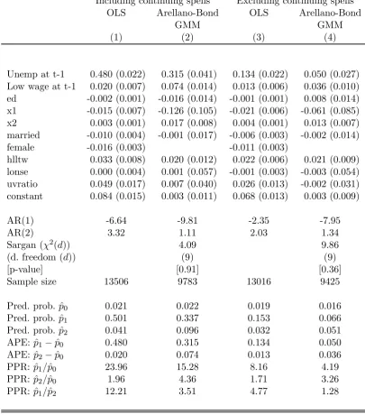
Columns 1 and 3 of Table 5 give OLS estimates of the DLP model including and
excluding continuing spells, comparable to columns 1 and 3 of Table 3. The results
are similar (once put on a comparable basis). The lagged unemployment and low
wage coefficients are similar to the APEs for the pooled probit estimator. Columns 2
and 4 give the Arellano-Bond GMM estimates using only lagged unemployment
vari-ables as instruments.31 The models pass the Arellano-Bond second-order residual
correlation test and the Sargan test of over-identifying restrictions.32 The estimates
of δ2 are not large, alleviating weak-instrument worries, and Blundell-Bond system
GMM estimates are similar to the Arellano-Bond ones. When the Anderson-Hsiao
IV estimator is used with either yt−2 or ∆yt−1 as instrument, the AR(2) test rejects
the null in both cases. Overall the evidence supports the use of the Arellano-Bond
GMM estimator.
31The 1-step estimates are presented, as advised by Doornik et al. (1999). The 2-step estimates
and their standard errors are very similar to the 1-step estimates presented. Using as additional instruments those used in Table 3 produces very similar estimates.
32If theω
it are not serially correlated, there should be evidence of significant negativefirst order
Focusing on column 4, the APEs for both lagged low wage and unemployment
are larger than those from the random effects probit model (Table 3, column 4).
Relative to the Heckman estimator, the APE of low wage att—1 has moved slightly
closer to that of unemployment at t—1: the gap is reduced from 0.020 to 0.014. The
effects of unemployment and low wage att—1 are again insignificantly different from
one another.33 In terms of predicting subsequent unemployment, the results of the
random effects probit estimators indicated that low wage employment holds a position
roughly half way between previous (but not continuous) unemployment and higher
wage employment. The GMM estimates shift this position to nearly three-quarters
of the way towards unemployment.
4.4
Low pay as a conduit to repeat unemployment
For those who experience repeat unemployment, the data do not provide information
on the wage rates of the job(s) held between the unemployment att—1 and that att.
An alternative way to investigate this involves using a second-order model to provide
an estimate for those unemployed att—2 and employed at t—1 of the impact of their
wage level att—1 on their probability of repeat unemployment at t.
The results above from all the dynamic random effects probit model estimators
(as well as the GMM estimators of the DLP model) show a strong degree of
agree-ment. The advantage of the Wooldridge estimator is that it requires only standard
random effects probit software, rather than specially written programs. It extends
in a relatively straightforward manner to the second-order case and is therefore the
most convenient to use to investigate the second-order model.
Column 2 of Table 6 gives the results for the Wooldridge estimator of the
second-order dynamic model. Column 1 gives the pooled probit estimates for comparison.
There are 9 combinations of states at t—2 and t—1. Dummy variables are included
for 8 of these with those higher paid at both t—2 and t—1 as the base group. Initial
values of both unemployment and low wage variables in both of thefirst two years are
included together with interactions between these and the time-averagedx-variables.
The coefficients for unemployment in both prior periods, unemployment followed
by low wage, low wage followed by unemployment and higher wage followed by
unem-ployment are all highly significant, of similar magnitude and insignificantly different
from one another. The test of coefficient equality between low wage and
unemploy-ment att—1 following unemployment at t—2 gives a p-value of 0.941. The coefficient
on unemployed followed by higher wage is in contrast not significantly different from
zero (a p-value of 0.092), i.e. this group’s probability of unemployment at t is not
significantly greater (at the 5% level) than that of those employed at a higher wage
at botht—2 and t—1.
The coefficient estimates imply an APE on the probability of unemployment at
t of unemployment at t—2 followed by low-wage employment at t—1 of 0.068, very
similar to that of unemployment in both periods. Someone unemployed at t—2 and
then low wage at t—1 is 3.2 times as likely to be unemployed at t as an equivalent
person higher wage in both periods. The APE of unemployment at t—2 followed
by higher-wage employment at t—1 is 0.019 (and insignificantly different from zero).
There is a significantly increased probability of being unemployed again at t having
been so at t—2 if the intervening point at t—1 was one of low wage employment, but
not if it was one of higher wage employment. Low wage jobs act as a conduit to
repeat unemployment. Higher wage jobs reduce the increased risk to insignificance.
5
Conclusions
This paper examines the extent of state dependence in individual unemployment and
the role played in this by low-wage employment. The three main findings are as
follows.
First, the aggregate state dependence in unemployment considerably overstates an
individual’s risk of repeat unemployment. Over half the measured state dependence
inter-vening employment) and about a third is removed when unobserved heterogeneity
and initial conditions are taken account of. Despite this, an individual unemployed
at t—1 who finds a job is still more than twice as likely to be unemployed again at
t as someone who was employed at t—1, but otherwise has the same observed and
unobserved characteristics; and this difference is statistically significant.
Second, low-wage employment att—1 has almost as large an adverse effect as
un-employment att—1 on the probability of employment att, and the difference between
the estimated effects is insignificant with all estimators.
Third, low-wage jobs act as the main conduit for repeat unemployment. Those
who get a better job reduce the increased risk of repeat unemployment to insignifi
-cance. The probability of re-entering unemployment for someone who gets a low-wage
job after a spell of unemployment is three times as great as that for someone with
the same observed and unobserved characteristics originally in employment.
In terms of future employment prospects, low-wage jobs are closer to
unemploy-ment than to higher paid jobs. The results in this paper suggest that not all jobs
are “good” jobs, in the sense of improving future prospects, and that low-wage jobs
typically do not lead on to better things. The results are consistent with the
hy-pothesis that a low-wage job does not augment a person’s human capital significantly
more than unemployment. If unemployed individuals’ employment prospects are to
be permanently improved, they need tofind jobs where they can augment their skills
(for example through on-the-job training) raise their productivity and move up the
pay distribution.
Acknowledgements
I am grateful to Wiji Arulampalam, Keith Cowling, Paul Gregg, Mary Gregory, Richard Jackman, Stephen Jenkins, Stephen Jones, Alan Manning, Robin Naylor, Steve Nickell, Odbjorn Rauum, John Rust, Sherwin Rosen, Jeremy Smith, Ian Walker, three anonymous referees and seminar participants at LSE, Warwick and the EALE / SOLE World Congress for helpful comments and discussions, and to the Leverhulme
Trust for financial support. The British Household Panel Survey data used in the
References
Acemoglu D. 2001. “Good jobs versus bad jobs”, Journal of Labor Economics, 19,
1—21.
Alessie R, Hochguertel S, van Soest A. 2005. “Ownership of stocks and mutual funds:
A panel data analysis”, Review of Economics and Statistics.
Anderson TW, Hsiao C. 1981. “Estimation of dynamic models with error
compo-nents”, Journal of the American Statistical Association, 76, 598—606.
Arellano M, Bond S. 1991. “Some tests of specification for panel data: Monte Carlo
evidence and an application to employment equations”, Review of Economic
Studies, 58, 277—97.
Arulampalam W. 1999. “A note on estimated coefficients in random effects probit
models”, Oxford Bulletin of Economics and Statistics, 61, 597—602.
Arulampalam W, Booth AL, Taylor MP. 2000. “Unemployment persistence”,Oxford
Economic Papers, 52, 24—50.
Baker M. 1997. “Growth-rate heterogeneity and the covariance structure of life-cycle
earnings”, Journal of Labor Economics, 15, 338—75.
Blanchard OJ, Diamond PA. 1994. “Ranking, unemployment duration, and wages”
Review of Economic Studies, 61, 417—34.
Blundell R, Bond S. 1998. “Initial conditions and moment restrictions in dynamic
panel data models”, Journal of Econometrics, 87, 115—43.
Burtless G. (ed.) 1990. A Future of Lousy Jobs? The Changing Structure of U.S.
Wages, Washington: Brookings Institute.
Butler JS, Moffitt R. 1982. “A computationally efficient quadrature procedure for
the one-factor multinomial probit model”, Econometrica,50, 761—4.
Chamberlain G. 1984. “Panel data”, inHandbook of Econometrics, ed. by Z. Griliches
and M. Intrilligator, Amsterdam: North-Holland.
Chay KY, Hyslop, DR. 2000. “Identification and estimation of dynamic binary
re-sponse panel data models”, U. of California Berkeley, Working Paper.
Clark KB, Summers LH. 1979. “Labour market dynamics and unemployment: a
reconsideration”, Brookings Papers on Economic Activity, 1, 13—60.
Corcoran M, Hill, MS. 1985. “Reoccurrence of unemployment among adult men”,
Journal of Human Resources, 20, 165—83.
Dickens R. 2000. “The evolution of individual male earnings in Great Britain: 1975— 94”, Economic Journal,110, 27—49.
Doornik JA, Arellano M, Bond S. 1999. “Panel data estimation using DPD for Ox”,
http://www.nuff.ox.ac.uk/users/doornik/.
Ellwood DT. 1982. “Teenage unemployment: permanent scars or temporary
blem-ishes?” in R. Freeman and D. Wise (eds.), The Youth Labour Market Problem:
Its Nature, Causes and Consequences, Chicago: U. of Chicago Press.
Flaig G, Licht G, Steiner V. 1993. “Testing for state dependence effects in a dynamic
model of male unemployment behaviour”, in H. Bunzel et al. (eds.) Panel Data
and Labour Market Dynamics, Amsterdam: North-Holland.
Flinn CJ, Heckman JJ. 1983. “Are unemployment and out of the labor force
Frijters P, Lindeboom M, van den Berg G. 2000. “Persistencies in the labour market”, working paper, Free University Amsterdam.
Gregg P. 2001. “The impact of youth unemployment on adult unemployment in the
NCDS”, Economic Journal, 111, F626—F653.
Gregg P, Wadsworth J. 2000. “Mind the gap, please: The changing nature of entry
jobs in Britain”, Economica, 67, 499—524.
Gregory M, Jukes R. 2001. “Unemployment and subsequent earnings: Estimating
scarring among British men 1984-94”, Economic Journal, 111, F607—25.
Heckman JJ. 1981a. “Heterogeneity and state dependence”, in S. Rosen (ed.) Studies
in Labor Markets, Chicago: University of Chicago Press (for NBER).
Heckman JJ. 1981b. “The incidental parameters problem and the problem of initial conditions in estimating a discrete time - discrete data stochastic process”, in
C.F. Manski and D. McFadden (eds.) Structural Analysis of Discrete Data with
Econometric Applications, Cambridge: MIT Press.
Heckman JJ. 2001. “Micro data, heterogeneity and the evaluation of public policy:
Nobel lecture”, Journal of Political Economy, 109, 673—748.
Heckman JJ, Borjas GJ. 1980. “Does unemployment cause future unemployment?
Definitions, questions and answers from a continuous time model of
heterogene-ity and state dependence”, Economica, 47, 247—83.
Hyslop DR. 1999. “State dependence, serial correlation and heterogeneity in
in-tertemporal labor force participation of married women”, Econometrica, 67,
1255—94.
Jacobson LS, LaLonde RJ, Sullivan DG. 1993. “Earnings losses of displaced
work-ers”, American Economic Review, 83, 685—709.
Keane M. 1994. “A computationally practical simulation estimator for panel data”,
Econometrica, 62, 95—116.
Kletzer LG. 1998. “Job displacement”, Journal of Economic Perspectives,12, 115—
36.
Layard R, Nickell S, Jackman R. 1991.Unemployment: Macroeconomic Performance
and the Labour Market, Oxford: Oxford University Press.
Low Pay Commission. 1998.The National Minimum Wage, First Report, Cm. 3796,
London: The Stationary Office.
Lynch LM. 1985. “State dependency in youth unemployment: A lost generation?”,
Journal of Econometrics,28, 71—84.
Lynch LM. 1989. “The youth labor market in the eighties: Determinants of
re-employment probabilities for young men and women”, Review of Economics
and Statistics, 71, 37—45.
McCormick B. 1990. “A theory of signalling during job search, employment efficiency
and “stigmatized” jobs”, Review of Economic Studies,57, 299—313.
Moffitt R, Gottschalk P. 1993. “Trends in the covariance structure of earnings in the
US: 1969—87”, Brown University Working Paper No. 9/93.
Muhleisen M, Zimmermann KF. 1994. “A panel analysis of job changes and
unem-ployment”, European Economic Review,38, 793—801.
Mundlak Y. 1978. “On the pooling of time series and cross section data”,
Narendranathan W, Elias P. 1993. “Influences of past history on the incidence of
youth unemployment: Empirical findings for the UK”, Oxford Bulletin of
Eco-nomics and Statistics, 55, 161—85.
Muhleisen M, Zimmermann KF. 1994. “A panel analysis of job changes and
unem-ployment”, European Economic Review,38, 793—801.
Omori Y. 1997. “Stigma effects of nonemployment”,Economic Inquiry,35, 394—416.
Stewart MB. 1999. “Low pay, no pay dynamics”, inPersistent Poverty and Lifetime
Inequality, HM Treasury Occasional Paper No. 10.
Stewart MB. 2005. “The Inter-related Dynamics of Unemployment and Low-wage Employment”, working paper, University of Warwick.
Stewart MB, Swaffield JK. 1999. “Low pay dynamics and transition probabilities”,
Economica, 66, 23—42.
Sweeney K. 1996. “Destinations of leavers from claimant unemployment”, Labour
Market Trends, October, 443—52.
Taylor MF. (ed.) 1996. British Household Panel Survey User Manual, Colchester:
U. of Essex.
Train KE. 2003. Discrete Choice Models with Simulation, Combridge Univ. Press.
Wooldridge JM. 2005. “Simple solutions to the initial conditions problem in dynamic,
nonlinear panel data models with unobserved heterogeneity”,Journal of Applied
Table 1
Unconditional and conditional probabilities of unemployment
Employed Unemployed
Unconditional at t-1 at t-1
All 0.044 0.023 0.491
Sex: Male 0.056 0.027 0.536
Female 0.031 0.019 0.399
Age left f-t education >16 0.035 0.021 0.380
≤16 0.054 0.025 0.570
Years potential experience >20 0.038 0.021 0.507
≤20 0.052 0.026 0.477
Married 0.037 0.020 0.493
Single 0.061 0.031 0.488
Health limits type or amount of work 0.090 0.044 0.592
Does not 0.040 0.022 0.473
Resident in London / South-East 0.043 0.023 0.496
Rest of country 0.045 0.024 0.488
UV ratio in TTWA >median 0.055 0.028 0.506
≤median 0.035 0.019 0.469
Notes:
1. Pooled data for BHPS waves 2-6 (1992-1996). 2. Sample size = 18,752.
Table 2
Variable definitions, means and standard deviations
Variable Description Mean (SD)
unemp Unemployed at time of interview (ILO/OECD definition) 0.048 (0.215) lwage Wage < £3.50 (adjusted to April 1997 using AEI) 0.078 (0.269)
ed Age completed full-time education 17.71 (2.906)
x1 Years potential labour market experience /10 2.176 (1.134)
x2 x12
married Married 0.690 (0.463)
female Female 0.459 (0.498)
hlltw Health limits type or amount of work 0.078 (0.269)
lonse London / South East 0.298 (0.457)
uvratio Unemployment-vacancy ratio in individual’s TTWA 0.184 (0.123)
Notes:
1. Pooled data for BHPS waves 1-6 (1991-1996). 2. Sample size = 23,491.
[image:28.595.113.532.500.678.2]Table 3
Dynamic Random Effects Probit Models for Unemployment Probability
Including continuing spells Excluding continuing spells
Pooled Heckman Pooled Heckman
probit estimator probit estimator
(1) (2) (3) (4)
Unemp at t-1 1.955 (0.056) 1.285 (0.115) 0.933 (0.090) 0.436 (0.146) Low wage at t-1 0.309 (0.082) 0.317 (0.103) 0.222 (0.091) 0.218 (0.107) ed -0.130 (0.051) -0.113 (0.056) 0.117 (0.114) 0.136 (0.131) x1 -0.193 (0.079) -0.361 (0.113) -0.314 (0.089) -0.405 (0.111)
x2 0.038 (0.016) 0.068 (0.023) 0.061 (0.018) 0.078 (0.023)
married 0.117 (0.161) 0.120 (0.186) 0.100 (0.186) 0.110 (0.209) female -0.229 (0.047) -0.335 (0.069) -0.212 (0.054) -0.249 (0.066) hlltw 0.278 (0.120) 0.340 (0.138) 0.493 (0.142) 0.575 (0.161) lonse -0.282 (0.360) -0.259 (0.402) -0.425 (0.382) -0.473 (0.422) uvratio -0.781 (0.398) -0.920 (0.475) -2.134 (0.472) -2.359 (0.548) a(ed) 0.100 (0.052) 0.066 (0.057) -0.140 (0.115) -0.166 (0.132) a(married) -0.293 (0.169) -0.393 (0.200) -0.242 (0.196) -0.274 (0.222) a(hlltw) 0.094 (0.152) 0.197 (0.186) -0.264 (0.188) -0.291 (0.217) a(lonse) 0.266 (0.363) 0.222 (0.408) 0.391 (0.384) 0.426 (0.426) a(uvratio) 1.829 (0.414) 2.373 (0.516) 3.229 (0.463) 3.720 (0.558) constant -1.250 (0.197) -1.094 (0.271) -1.187 (0.222) -1.257 (0.273)
λ 0.383 (0.062) 0.262 (0.069)
θ 1.033 (0.175) 0.936 (0.310)
Log likelihood -2732.81 -2703.74 -1981.72 -1970.22
GOF-statistic 137.60 63.04 325.71 61.02
[p-value] 0.000 0.475 0.000 0.547
Sample size 13506 17229 13016 16607
Pred. prob. pˆ0 0.029 0.032 0.035 0.038
Pred. prob. pˆ1 0.447 0.181 0.155 0.072
Pred. prob. pˆ2 0.052 0.052 0.052 0.053
APE: pˆ1−pˆ0 0.419 0.150 0.130 0.035
APE: pˆ2−pˆ0 0.023 0.020 0.017 0.015
PPR: pˆ1/pˆ0 15.68 5.76 4.43 1.92
PPR: pˆ2/pˆ0 1.82 1.65 1.49 1.40
PPR: pˆ1/pˆ2 8.61 3.49 2.97 1.37
Notes:
1. Standard errors in brackets.
2. The variable a(x) is the mean over time of the variable x. 3. All models also contain year dummies.
4. log L and GoF statistics for columns (1) and (3) combined with period 1 standard probits. 5. Sample sizes given for columns (1) and (3) are for periods 2—6 only.
6. GoF p-value based on χ2(63).
7. pˆ0, pˆ1, pˆ2 = predicted probabilities of unemployment at t given higher wage, unemployed, low wage at t-1 respectively.
Table 4
Alternative Estimators of Dynamic Random Effects Probit Model
Wooldridge Discrete AR(1) Heterogeneous
estimator mixture errors slope model
(1) (2) (3) (4)
Unemp at t-1 0.435 (0.152) 0.423 (0.152) 0.445 (0.327) 0.404 (0.476) Low wage at t-1 0.211 (0.106) 0.220 (0.108) 0.217 (0.102) 0.214 (0.106)
ed 0.135 (0.131) 0.136 (0.130) 0.127 (0.127) 0.136 (0.066)
x1 -0.393 (0.110) -0.417 (0.113) -0.382 (0.104) -0.403 (0.108)
x2 0.077 (0.022) 0.081 (0.023) 0.074 (0.021) 0.078 (0.022)
married 0.118 (0.208) 0.112 (0.210) 0.108 (0.203) 0.107 (0.209) female -0.230 (0.065) -0.248 (0.068) -0.236 (0.062) -0.240 (0.067) hlltw 0.567 (0.160) 0.575 (0.163) 0.552 (0.155) 0.570 (0.161) lonse -0.478 (0.422) -0.469 (0.429) -0.468 (0.408) -0.476 (0.422) uvratio -2.278 (0.540) -2.416 (0.576) -2.286 (0.523) -2.332 (0.544) a(ed) -0.156 (0.132) -0.166 (0.131) -0.156 (0.128) -0.166 (0.066) a(married) -0.268 (0.222) -0.275 (0.222) -0.268 (0.214) -0.272 (0.222) a(hlltw) -0.244 (0.220) -0.261 (0.218) -0.280 (0.208) -0.304 (0.217) a(lonse) 0.432 (0.427) 0.417 (0.433) 0.427 (0.412) 0.427 (0.426) a(uvratio) 3.798 (0.558) 3.809 (0.615) 3.571 (0.525) 3.729 (0.558)
constant -1.203 (0.270) -1.250 (0.269)
λ 0.235 (0.069) 0.193 (0.060)
θ 1.099 (0.534) 1.078 (0.475) 0.897 (0.413)
Point 1 -4.416 (3.928)
Point 2 -0.805 (0.352)
Point 3 0.352 (0.554)
Prob 1 0.402 (0.179)
Prob 2 0.577 (0.159)
Prob 3 0.021 (0.033)
ρ 0.054 (0.171)
σ 0.557 (0.126)
σ2 0.773 (0.333)
ρα -0.125 (0.483)
Log likelihood -1977.76 -1969.91 -1969.65 -1967.12
GOF-statistic 57.23 57.13 74.45 67.38
[p-value] 0.681 0.685 0.153 0.330
Sample size 13016 16607 16607 16607
Pred. prob. pˆ0 0.035 0.037 0.037 0.032
Pred. prob. pˆ1 0.068 0.068 0.075 0.061
Pred. prob. pˆ2 0.049 0.051 0.053 0.046
APE: pˆ1−pˆ0 0.033 0.031 0.037 0.029
APE: pˆ2−pˆ0 0.014 0.015 0.016 0.014
PPR: pˆ1/pˆ0 1.95 1.85 2.00 1.90
PPR: pˆ2/pˆ0 1.39 1.39 1.42 1.42
PPR: pˆ1/pˆ2 1.40 1.33 1.41 1.34
Table 5
GMM estimation of Dynamic LPM for Unemployment Probability
Including continuing spells Excluding continuing spells
OLS Arellano-Bond OLS Arellano-Bond
GMM GMM
(1) (2) (3) (4)
Unemp at t-1 0.480 (0.022) 0.315 (0.041) 0.134 (0.022) 0.050 (0.027) Low wage at t-1 0.020 (0.007) 0.074 (0.014) 0.013 (0.006) 0.036 (0.010) ed -0.002 (0.001) -0.016 (0.014) -0.001 (0.001) 0.008 (0.014) x1 -0.015 (0.007) -0.126 (0.105) -0.021 (0.006) -0.061 (0.085)
x2 0.003 (0.001) 0.017 (0.008) 0.004 (0.001) 0.013 (0.007)
married -0.010 (0.004) -0.001 (0.017) -0.006 (0.003) -0.002 (0.014)
female -0.016 (0.003) -0.011 (0.003)
hlltw 0.033 (0.008) 0.020 (0.012) 0.022 (0.006) 0.021 (0.009) lonse 0.000 (0.004) 0.001 (0.057) -0.001 (0.003) -0.003 (0.054) uvratio 0.049 (0.017) 0.007 (0.040) 0.026 (0.013) -0.002 (0.031) constant 0.084 (0.015) 0.003 (0.011) 0.068 (0.013) 0.003 (0.009)
AR(1) -6.64 -9.81 -2.35 -7.95
AR(2) 3.32 1.11 2.03 1.34
Sargan (χ2(d)) 4.09 9.86
(d. freedom (d)) (9) (9)
[p-value] [0.91] [0.36]
Sample size 13506 9783 13016 9425
Pred. prob. pˆ0 0.021 0.022 0.019 0.016
Pred. prob. pˆ1 0.501 0.337 0.153 0.066
Pred. prob. pˆ2 0.041 0.096 0.032 0.051
APE: pˆ1−pˆ0 0.480 0.315 0.134 0.050
APE: pˆ2−pˆ0 0.020 0.074 0.013 0.036
PPR: pˆ1/pˆ0 23.96 15.28 8.16 4.19
PPR: pˆ2/pˆ0 1.96 4.36 1.71 3.26
PPR: pˆ1/pˆ2 12.21 3.51 4.77 1.28
Notes:
1. Robust standard errors in brackets. 2. All models also contain year dummies.
3. pˆ0, pˆ1, pˆ2 = predicted probabilities of unemployment at t given higher wage, unemployed, low wage at t-1 respectively.
Table 6
2nd-order Dynamic Random Effects Model
Pooled Wooldridge
probit estimator
(1) (2)
UU 1.217 (0.117) 0.673 (0.201)
UL 1.099 (0.178) 0.690 (0.217)
UH 0.616 (0.121) 0.262 (0.156)
LU 0.962 (0.252) 0.656 (0.293)
HU 0.888 (0.135) 0.740 (0.189)
LL 0.236 (0.128) 0.083 (0.189)
LH 0.214 (0.140) 0.132 (0.168)
HL 0.263 (0.154) 0.195 (0.170)
ed -0.039 (0.035) -0.051 (0.039)
x1 -0.339 (0.090) -0.330 (0.098)
x2 0.072 (0.019) 0.073 (0.020)
married -0.048 (0.197) -0.060 (0.204) female -0.188 (0.056) -0.196 (0.060)
hlltw 0.449 (0.144) 0.416 (0.147)
lonse -1.019 (0.404) -1.034 (0.414) uvratio 0.040 (0.619) 0.057 (0.634)
a(ed) 0.033 (0.034) 0.056 (0.039)
a(married) -0.106 (0.208) -0.064 (0.218) a(hlltw) -0.147 (0.188) -0.019 (0.201) a(lonse) 1.045 (0.406) 1.045 (0.418) a(uvratio) 0.523 (0.714) 0.661 (0.771) constant -1.664 (0.232) -1.962 (0.267)
σu 0.149 (0.293)
λ 0.022 (0.084)
Log likelihood -1198.03 -1171.29
Sample size 11461 11461
APE: UU 0.168 0.066
APE: UL 0.141 0.068
APE: UH 0.057 0.019
PPR: UU 6.92 3.11
PPR: UL 5.97 3.19
PPR: UH 2.99 1.61
Notes:
1. Lagged status variables: U=unemp, L=low wage, H=High wage. 2. 1st. letter in lagged status code is status at t-2, 2nd. is that at t-1. 3. All models also contain year dummies.