Instrument design in UV polarised spectroscopy

A Thesis Submitted for the Degree of PhD at the University of Warwick

http://go.warwick.ac.uk/wrap/51549

This thesis is made available online and is protected by original copyright. Please scroll down to view the document itself.

Instrument Design in UV Polarised

Spectroscopy

Daniel Waldron

Submitted in partial fulfilment of the

requirements for the degree of Doctor of

Philosophy

Contents (Outline)

List of Figures

List of Tables

Acknowledgements

Dedication

Declaration

Abstract

Abbreviations

Chapter 1: Introduction

Chapter 2: Development of capillary circular dichroism spectroscopy and discussion

of capillary optics

Chapter 3: Development of an etched cuvette of well-defined path-length for

circular dichroism spectroscopy

Chapter 4: Development of automated multi-sample circular dichroism

(AMS-CD)

Contents (Detailed)

Contents (Outline)...2

Contents (Detailed) ...3

List of figures...6

List of tables...17

Acknowledgements...18

Dedication ...20

Declaration...21

Abstract ...22

Abbreviations...23

CHAPTER ONE Introduction...25

Summary...26

1.1 Chemical basis of biological systems...27

1.1.1 DNA...28

1.1.2 RNA ...30

1.1.3 Proteins ...30

Protein organisation and structure ...31

Secondary structure bonding motifs ...32

1.1.4 Lipids, membranes and bilayers ...35

1.1.5 Methods for determining the structure of biological macromolecules ...36

1.2 Spectroscopy ...37

1.2.1 UV spectroscopy...39

1.2.2 Circular Dichroism...40

Physical basis for circular dichroism spectroscopy ...41

DNA Circular Dichroism...43

Protein Circular Dichroism...43

Flexibility of circular dichroism as an analysis method ...46

Instrumentation ...46

Instrument parameters...48

1.2.3 Linear Dichroism ...49

1.3 References ...51

CHAPTER TWO Development of capillary circular dichroism spectroscopy .54 Summary...55

2.1 Introduction ...56

2.1.1 Cuvette circular dichroism...57

2.1.2 Capillary circular dichroism ...58

2.2 Instrument development...58

2.2.1 Initial design...58

2.2.2 Capillary optics ...62

2.2.3 Spectrophotometer design– a case for precision optical engineering in CD applications...66

2.2.4 Multiple optical elements reduce photon flux ...68

2.2.5 caCD ‘alignment’ cell ...69

2.2.6 caCD cell final design...74

2.3 Materials and methods ...77

Standard Operating Procedure: ...78

Step 1: Alignment of the light beam ...80

Step 2: Sample loading ...80

Step 3: Optical alignment of the capillary ...81

Step 4: Acquisition of spectrum...81

Step 5: Cleaning of the capillary...82

2.4 Results and Discussion...82

2.4.1 Capillary CD quality compared to Cuvette CD ...82

Na[Co(EDDS)].H2O...83

Lysozyme...84

Concanavalin A...85

Progesterone...86

2.4.2 New experiments facilitated by the development of CaCD...87

YOYO-1 DNA binding...87

CoEDDS scattering experiment...90

2.5 Conclusion...92

2.6 References ...93

CHAPTER THREE Development of an etched cuvette of well-defined path-length for circular dichroism spectroscopy...95

Summary...96

3.1 Introduction...97

3.1.1 Rationale for precision CD cuvettes ...97

3.2 Materials and methods ...97

3.2.1 Materials ...97

3.2.2 Cuvettes...98

3.2.3 Quartz flats...98

3.2.4 Quartz Etching ...98

3.2.5 Methods for assessing the flatness of quartz surfaces ...98

3.2.6 Machining ...101

3.3 Results and Discussion...101

3.3.1 Currently available cuvettes...101

3.3.2 Producing cells of known depth using optical flats ...103

3.3.3 Etching mask...105

3.3.4 Assessment of the surface quality of the etched flat...106

3.3.5 Sample loading...110

3.3.6 Sample holder ...111

3.3.7 CD spectroscopic data for etched and standard cuvettes ...113

3.4 Conclusions ...117

3.5 References ...118

CHAPTER FOUR Development of Automated multi-sample Circular Dichroism Spectroscopy ...120

(AMS-CD) ...120

Summary...121

4.1 Introduction ...122

4.1.1 The un-harnessed potential of circular dichroism...122

4.1.2 Capillary flow circular dichroism ...122

4.1.3 Alternative sample loading methodologies- single sample injection and queued flow...123

Queued flow AMS-CD ...124

4.2.1 Queued sample injection instrumentation and materials ...124

4.2.2 Single sample injection instrumentation...125

4.2.3 Cleaning methods...125

4.2.4 Consumables...126

4.3 Results and Discussion...126

4.3.1 Development of AMS-CD flow optic...126

4.3.2 Queued sample injection AMS-CD development...128

Integration of AS 2055 intelligent auto-sampler ...129

Programming the AS 2055 intelligent auto-sampler and PU-1580 HPLC pump ...131

Queued sample injection testing ...133

Queued sample AMS-CD applications...139

4.3.3 Single-sample injection AMS-CD development ...146

ASTRID light source ...148

Single-sample injection capillary holder ...149

Single- sample injection testing...151

4.4 Conclusions ...158

4.5 References ...160

CHAPTER FIVE Linear Dichroism of Biological Systems ...162

Summary...163

5.1 Introduction ...164

5.1.1 Linear dichroism as a means of analysing biological systems .164 5.1.2 Bacteria ...164

5.1.3 Whole organism linear dichroism...165

5.1.4 LD from other sources in the cell ...167

5.2 Materials and methods ...168

5.2.1 Materials ...168

5.2.2 Methods...168

B. Subtilis cell culture preparation...168

Flagella Preparation ...169

Electron Microscopy sample preparation ...169

Instrumentation ...170

5.3 Results ...171

5.3.1 Bacillus Subtilis ...171

5.3.2 Flagella association...177

5.4 Conclusions ...178

5.5 References ...179

CHAPTER SIX Conclusions & Future Work...181

Summary...182

Conclusions...183

Future work...187

Appendix 1- Capillary circular dichroism paper ...189

List of figures

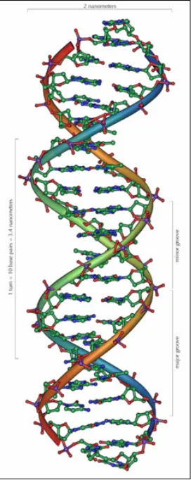
Figure 1.1: DNA double Helix. Image by Michael Ströck, under the GNU Free Documentation License, availible at http://commons.wikimedia.org. Figure 1.2: Different types of DNA. From left to right: A-DNA, B-DNA and

Z-DNA. Note how the structures, whilst all being helical, vary widely with A and B forming a wider, shorter double helix than is observed in Z-DNA. Image created by Richard Wheeler, available at

http://commons.wikimedia.org.

Figure 1.3: Molecular Structure of an α-helix. Image (a) shows the overall

structure of the helix, whilst image (b) shows which residues associate with each other to form the helix. Image (c) shows the helix from a covalent bond perspective, highlighting the orientation of various chemical groups within. (Image taken from C. I. Branden,J. Tooze, Introduction to Protein Structure).

Figure 1.4: Different types of helix; the α-helix, 3.10 helix and π-helix. The

different types of helical structure are formed from a change in the number of residues that comprise each turn. Image taken from http://www.cryst.bbk.ac.uk/PPS2/course/section8/ss-960531_5.html. Figure 1.5: Parallel and anti-parallel β-sheet structures. (Image taken from

http://wiz2.pharm.wayne.edu/biochem/prot.html)

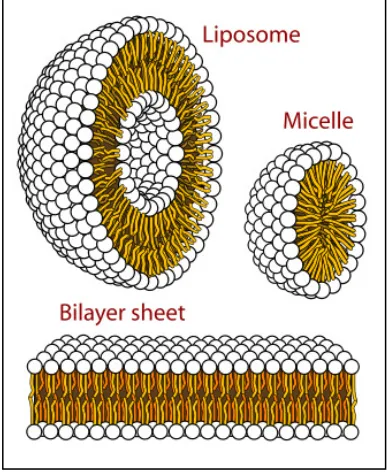
Figure 1.6: Different cellular forms of phospholipid layers. Image used with permission of Mariana Ruiz Villarreal from

http://commons.wikimedia.org

Figure 1.7: Aromatic absorption spectrum of tryptophan, tyrosine and

phenylalanine. Figure from Circular Dichroism and Linear Dichroism (Rodger and Nordén, 1997).

Figure 1.8: Circularly polarised light creation using wave interference. Image created using the wave modelling program EMANIM, developed by András Szilágyi (program available free at

Figure 1.9: Difference in electron redistribution upon excitation between a chiral and non- chiral system. Electron movement in a chiral system will always be of a helical nature, whilst in an achiral system movement is always planar. Image taken from ‘Circular Dichroism and Linear Dichroism’13. Figure used with permission.

Figure 1.10: CD spectra of the major secondary structure types. Solid line, α-helix;

long dashed line, anti-parallel β-sheet; dotted line, type I β-turn; cross

dashed line, poly proline II helix; short dashed line irregular structure. It is important to note that whilst termed ‘random coil’, is used the structure of such molecules is still highly ordered, hence the generation of a reproducible CD spectrum. Figure taken from the paper ‘How to study Proteins by Circular Dichroism’ by Kelly et al.

Figure 1.11: Diagram of the optical bench within a J-800 series CD spectrophotometer. Light of all wavelengths is generated from the xenon lamp, before being manoeuvred through two monochromators (the 1st being between S1 & S2, the 2nd between S2 & S3). These two monochromators (more commonly referred to as a double monochromator) is very effective at reducing stray light within an optical system. The prisms within each monochromator, in addition to selecting a wavelength of light are also axially orientated, generating linearly polarised light that is easier to modulate. All reflection within the system is achieved using aluminium mirrors. Figure from Model J-800 CD spectrometer Hardware/Function manual (2006) by Jasco. Figure used with permission of Jasco UK.

Figure 1.12: Experimental set-up for linear and circular dichroism (image taken from Hinds Instruments application note on photoelastic modulators, by T.C. Oakberg (an excellent source, free download of the application note at

http://www.hindsinstruments.com/wp-content/uploads/LinearCircular_Dichroism.pdf).

between the rod and capillary that the sample is contained within. Image taken from www.kromatek.co.uk.

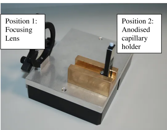
Figure 2.1: The focusing lens of the caCDRM instrument. Note that the lens is positioned precisely in the centre of the capillary.

Figure 2.2: caCDRM image showing the slide-way of the instrument. The base-plate features a groove, where various optical components can slot into.

Figure 2.3: Na [Co (Edds)].H2O at 0.55 mM spectra acquired through both cuvette

CD and caCD. The caCD spectra were acquired using the Marrington design of caCD base plate. The path-length of the capillary was 1.12 mm, determined through analysis with potassium dichromate. Capillary spectra scaled using a 0.892 correction factor to allow for differences in path-length. The path-length of the cuvette was 1 mm, verified via analysis with potassium dichromate.

Figure 2.4: ‘Many faces of light: As Newton Saw it, With Some Magic Tricks’ lecture given by Prof. U. Mallik 14/02/05.

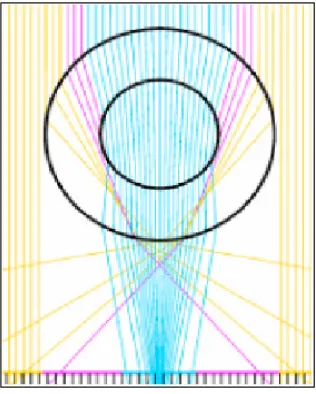
Figure 2.5: Capillary Optics. Blue lines represent light that passes through the internal diameter of the capillary. Pink lines represent light that interacts with the internal bore of the capillary but is still optically net divergent. Yellow lines represent light that does not interact at all with the internal bore of the capillary, creating a high degree of divergence. Image used with permission of Paraytec Ltd.

Figure 2.6: Graph showing the relationship between slit-width and wavelength for a J-800 series spectrophotometer (data plotted from Jasco technical notes for the J800 series spectrophotometer).

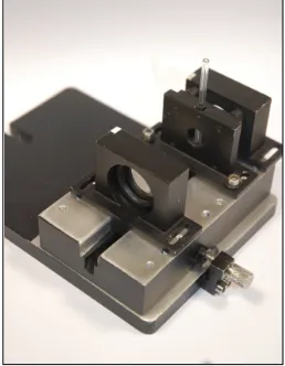
Figure 2.7: The alignment caCD cell, including lens holder. The design for this cell was simple and very cost effective. However, difficulties with data reproducibility marred the cell design.

Figure 2.8: Diagram showing the effect on the light beam as it interacts with the capillary.

Figure 2.9: Na [Co (Edds)].H2O 0.55 mM spectra acquired through both cuvette

scaled using a 0.892 correction factor to facilitate comparison between the spectra. The path-length of the cuvette was 1 mm, verified with potassium dichromate.

Figure 2.10: Diagram to illustrate the effect of longitudinal chromatic aberration on a light beam. (Image taken from

http://en.wikipedia.org/wiki/File:Lens6a.svg)

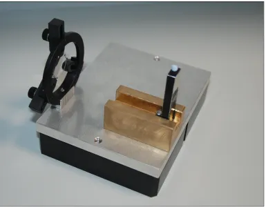
Figure 2.11: Final design for the caCD cell. Building on the concepts of the alignment cell, this cell locks all the optical components in place to consistently generate high quality spectra.

Figure 2.12: Reflected light between two surfaces. From left to right: As the light beam hits a transmitting surface, some of the light is reflected backwards. Part of this light is in turn reflected, creating additional optical changes.

Figure 2.13: Na [Co (Edds)].H2O 0.55 mM spectra acquired through both cuvette

CD and caCD. The caCD spectra were acquired using the final design of caCD base plate. The path-length of the capillary was 1.12 mm, determined using potassium dichromate. Spectra scaled using a 0.892 correction factor to account for length differences. The path-length of the cuvette was 1 mm, verified with potassium dichromate. Figure 2.14: The caCD sample cell.

Figure 2.15: CD spectra, with separate HT trace, of Na [Co (EDDS)].H2O (0.55

mM in water) in a cuvette (1 mm path length) and capillary (1.12 mm path length, data divided by 1.12 to facilitate comparison). The RR spectra have been multiplied by minus 1 for ease of comparison. Figure 2.16: CD spectra of lysozyme (0.1 mg/ml) in a cuvette of 1 mm path length).

Capillary before cuvette denotes CD measured in a cuvette located before a water-filled capillary. Similarly, capillary after cuvette denotes a spectrum measured in a cuvette placed after the light beam has passed through a water-filled capillary.

Figure 2.18: CD spectra, with HT traces overlaid, of progesterone (0.1 mg/ml) in a cuvette (1 mm path length) and capillary (1.16 mm path length, data divided by 1.16 to facilitate comparison).

Figure 2.19: CD spectra, with HT traces overlaid, of calf thymus DNA (200 µM) in a cuvette (1 mm path length) and capillary (1.16 mm path length, data divided by 1.16 to facilitate comparison). YOYO-1 was added to the DNA prior to be being placed in the capillary.

Figure 2.20: YOYO exciton CD spectra, with Ht traces overlaid, of YOYO-1 bound to 200 µM calf thymus DNA in a capillary (1.16 mm path length). YOYO-1 was added to the DNA prior to be being placed in the capillary.

Figure 2.21: CD spectra, with HT traces overlaid, of 0.5 mM S,S COEDDS in the presence of 100 nm polymer spheres.

Figure 2.22: CD spectra, with HT traces overlaid, of 0.5 mM R,R COEDDS in the presence of 100 nm polymer spheres.

Figure 3.1: Figure illustrating types of interference pattern generated by different surface finishes. Image taken from ‘Optical flat manual’ Edmund Optics Worldwide.

Figure 3.2: Interferometry pattern of a 1 mm thermally annealed quartz cuvette. The top of the pattern shows evidence of optical flaws (in this instance, a convex surface), reducing the accuracy of the cuvette. This effect is small in a 1 mm cuvette, but can have a big impact when designing cuvettes at the micron level of accuracy.

Figure 3.3: Interferometry pattern of a ‘flat’ component of a 10 micron path length Starna cuvette. The ‘saddle’ interference pattern observed here is quite rare, showing a region of overlapping concave and convex surfaces. The errors shown here are well into the micron level of surface error, based on the inference pattern observed here.

Figure 3.5: The etching rig female component, before (left) and after (right) the etching process. It should be highlighted that after etching, two of the heads of the screws had been so undermined by acid attack that they disintegrated upon removal from the HF solution. Figure 3.6: (a) Bottom face, (b) top face and (c) side view of the etching rig machined on a lathe in black nylon. The recess in the centre of the bottom was been machined to create a push-fit for a 1 inch diameter cylindrical quartz flats.

Figure 3.7: Interference pattern of an etched flat. Note the band pattern on both sides of the channel, where optical flatness has been retained.

Figure 3.8: WYKO image of a 6.5 µm etched flat channel / plain surface. The surface finish of both the etched and non-etched components is of exceptional quality, in terms of surface roughness and sharpness of interface. There is very little evidence of

undercutting or smoothing at the interface, proving the efficacy of the acid mask.

Figure 3.9: Assembled etched cuvette inside the sample cell holder. The interference pattern of the two flats can be clearly seen, identifying the surfaces of the two pieces of quartz as being optically flat.

Figure 3.10: UV / Visible spectrum absorbance spectrum of the etched cell. The spectrum was acquired under the following conditions: Bandwidth 1 nm, data pitch 0.2 nm, scan speed 100 nm/min. Figure 3.11: UV/Vis K2CrO4 path-length determination. A 0.2 M solution

was used to test the micron path-length cuvettes, whilst a 0.002 M solution was used for the 1 mm path-length cuvette.

Parameters for the UV/Vis analysis were: bandwidth 1 nm, data pitch 0.5 nm, speed 100 nm/min.

Figure 3.12: Etched cuvette holder assembly side view schematic. An

Figure 3.13: Etched cuvette base-plate side view schematic. Light source in this instance would move from left to right.

Figure 3.14: Etched cuvette front view schematic. Light source in this instance would move through plane of the optical iris.

Figure 3.15: Sample holder unit. Right: quartz optical flats assembled and capped with a black rubber ‘O’ ring. Middle: Optical flat unit fitted inside the cell holder. Left: assembled unit indicating screw that facilitates positioning of the unit in the light path. Figure 3.16: Na [Co (Edds)].H2O spectra for 6.6 micron etched cuvette (55

mM) and 1 mm cuvette (0.55 mM). Etched cuvette spectra have been adjusted for concentration and path-length. Parameters used were 100 nm / min scan speed; bandwidth 1 nm, step size 0.2 nm for the etched cell and 100 nm / min scan speed, bandwidth 1 nm, step size 0.5 nm for the 1 mm cuvette.

Figure 3.17: Concanavalin A spectra for 6.6 micron etched cuvette (10 mg / ml) and 1 mm cuvette (0.1 mg / ml). Etched cuvette spectra have been adjusted for path-length. Parameters used were 100 nm / min scan speed, bandwidth 1 nm, step size 0.2 nm.

Figure 3.18: Ovalbumin spectra for 6.6 micron etched cuvette (10 mg / ml) and 1 mm cuvette (0.1 mg / ml). Etched cuvette spectra have been adjusted for path-length.

Figure 4.1: Jasco J-715 spectrophotometer. Note the long tubular detector on the right.

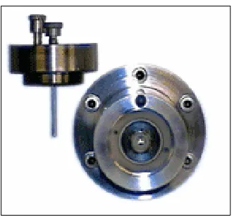
Figure 4.2: AMS-CD flow optic holder.

Figure 4.3: Brass plates that hold the capillary optic in place. Blu Tack® was used to secure the PEET tubing that connects the capillary optic to the HPLC auto-sampler.

Figure 4.4: Averaged CD spectrum and HT of 48 water samples, in order to verify spectral fidelity of the AMS-CD set-up. CD parameters were as follows: Bandwidth 2 nm, response 1 second, data pitch 0.2 nm, 2 accumulations. Error bars are given to one standard deviation.

Figure 4.6: The Jasco AS-2055 HPLC auto-sampler with integrated PU-1580 HPLC pump, modified for use with a CD spectrophotometer. Figure 4.7: Mean CD spectrum of ovalbumin (0.1 mg/ml) Capillary spectra

(not baseline subtracted). Data were acquired on a J-715 spectrophotometer using the QS AMS-CD system. CD

parameters were as follows: Bandwidth 2 nm, response 1 second, data pitch 0.2 nm, 2 accumulations. All error bars display +/- one standard deviation of the mean.

Figure 4.8: Overlay of forty eight Ovalbumin (0.1 mg/ml) Cuvette spectra (not baseline subtracted). Data was acquired on a J-715

spectrophotometer using a Starna 1 mm cuvette. CD parameters were as follows: Bandwidth 2 nm, response 1 second, data pitch 0.2 nm, 2 accumulations.

Figure 4.9: Time course measurement of 11 sample injections of 0.1 mg/ml lysozyme preceded by water injections, under repeated injection at 225 nm using QS AMS-CD. The path-length of the capillary in this instance was 1.1.mm. (determined through use of

potassium chromate). The CD signal accumulation of water corresponds to the upper bunches of readings; lysozyme corresponds to the lower bunches.

Figure 4.10: QS AMS-CD spectra of lysozyme (0.5 mg/ml baseline

subtracted). The image above shows 48 lysozyme spectra, with a water baseline recorded after each lysozyme sample. CD

parameters were as follows: Bandwidth 2 nm, response 1 second, data pitch 0.2 nm, 2 accumulations.

Figure 4.11: QS AMS-CD lysozyme spectra (0.5 mg/ml, baseline subtracted). Spectra that were more than 25% away from the mean ellipticity at 195 nm were omitted. CD parameters were as follows: Bandwidth 2 nm, response 1 second, data pitch 0.2 nm, 2 accumulations.

Figure 4.13: QS-AMS CD data of 1st mixed refolding agent screen. HRP concentration for all samples was at 0.5 mg / mL of denatured HRP protein. CD parameters were as follows: Bandwidth 2 nm, response 1 second, data pitch 0.2 nm, 2 accumulations.

Figure 4.14: QS-AMS CD data of 2nd mixed refolding agent screen. HRP concentration for all samples was at 0.5 mg / mL of denatured HRP protein. CD parameters were as follows: Bandwidth 2 nm, response 1 second, data pitch 0.2 nm, 2 accumulations.

Figure 4.15: QS-AMS CD data of 3rd mixed refolding agent screen. HRP concentration for all samples was at 0.5 mg / mL of denatured HRP protein. CD parameters were as follows: Bandwidth 2 nm, response 1 second, data pitch 0.2 nm, 2 accumulations.

Figure 4.16: CD spectrum comparison between four best performing refolding agents against the three worst (by activity), all data acquired by QS-AMS CD. All HRP concentrations are at 0.5 mg / mL. For the purposes of comparison, the water CD spectrum is using un-denatured HRP.

Figure 4.17: ELISA activity assay data for the best vs. worst performing refolding agents. Water baseline is marked as ‘standard’ (data acquired by Lisa Tuckley, Birmingham University).

Figure 4.18: Jasco ASU 605 auto sampler. A robot arm can move in the X,Y and Z directions, with an external pump being used to actually inject samples into the capillary optic.

Figure 4.19: NCS-609 Syringe pump.

Figure 4.20: Schematic of the ASTRID light source. Image available at

http://commons.wikimedia.org/wiki/Main_Page.

Figure 4.21: Masked capillary holder for the SSI AMS-CD apparatus that was tested at the ASTRID beam-line, Aarhus.

Figure 4.23: The capillary holder flow optic interface with the ASTRID CD1 beam line. Samples that were injected into the capillary would flow from left to right. The capillary flow optic was slotted into place in front of the detector, before being secured into place using electrical tape.

Figure 4.24: Capillary holder and sample lines after integration into the ASTRID CD1-beamline. The detector has been removed to show the location of the capillary optic inside the sample chamber.

Figure 4.25: Fully integrated and assembled SSI AMS CD device at the CD1 beam-line at ASTRID, Aarhus University. The cylinder wrapped in aluminium foil (top right) is the beam line link to the storage ring.

Figure 4.26: CD spectra of 0.1 mg / ml Ovalbumin, (capillary path-length 1.1 mm). All CD spectra were acquired at the ASTRID synchrotron light source at ISA, Aarhus University.

Figure 4.27: CD spectra of 0.1 mg / ml lysozyme (capillary path-length 1.1 mm). All CD spectra were acquired at the ASTRID synchrotron light source at ISA, Aarhus University.

Figure 4.28: CD spectra of 0.2 mg / ml Horse Radish Peroxidase (capillary path-length 1.1 mm). All CD spectra were acquired at the ASTRID synchrotron light source at ISA, Aarhus University. Figure 4.29: CD spectra of 0.1 mg / ml Concanavalin A (capillary path-length

1.1 mm). All CD spectra were acquired at the ASTRID synchrotron light source at ISA, Aarhus University.

Figure 5.1: LD spectra of Bacillus Subtilis in Luria Broth. Final LD signal is shown in blue. Figure taken from the thesis of Dr. Adair Richards ‘Taking the fight to the Superbugs: Interactions of Synthetic DNA-binding Metallomolecules with Biological Systems’. Figure used with permission.

Figure 5.2: LD spectrum of B. Subtilis at an A280 concentration of 1.5 OD

(baseline subtracted). The phosphate buffer baseline is included here to facilitate comparison. The bacteria were buffered in pH 7, 0.1 M phosphate solution. Orientation of the sample was achieved using a Couette LD cell under standard conditions.

Figure 5.3: E.M. image of B.Subtilis. The sample was taken from a solution of LB

media, rather than agar to properly reflect the number of flagella present per bacterium as measured by other methods. The large black object towards the bottom left of the image is a B.Subtilis bacterium,

whilst its flagella can be most clearly seen centre left and centre right, protruding from the rear of the bacterium

Figure 5.4: E.M. image of cell extract post homogenisation. The sample was taken from the suspension of the homogenised solution after

centrifugation. This fraction contains cell debris, as well as individual flagella (the long thin objects within the image, the best example being in the top right hand corner of the E.M. image).

Figure 5.5: E.M. image of purified flagella, taken from a re-suspension of the pellet produced via ultra-centrifugation.

Figure 5.6: LD spectrum of 0.25 OD Flagella.

Figure 5.7: LD spectrum of B. Subtilis under different flow conditions. All B.

Subtilis spectra were acquired at an Å280 concentration of 1.5 OD The LD spectra of A 0.25 OD couette aligned purified flagella and the original Couette LD B. Subtilis have been added to the figure for comparison.

List of tables

Table 2.1: Table displaying the change in slit size with wavelength in a J-800 spectrophotometer over a consistent 1 nm bandwidth.

Table 2.2: Table showing the effect of chromatic aberration on the focal length of a 100 mm DCX lens. A J-600 spectropolarimeter was used as the light source for these measurements. Focal point determined using white fluorescent paper.

Table 3.1 Etch time to depth of channel created.

Table 4.1 Table 4.1: Dichroweb analysis of SSI AMS-CD data compared against cuvette data, collected at the ASTRID beam-line. CD data sets used for analysis are the same as those presented in figures 4.26 – 4.29.

Table 4.2 Table 4.2: Dichroweb secondary structure analysis of SSI AMS-CD data compared against cuvette data, collected at the ASTRID beam-line. CD data sets used for analysis are the same as those presented in figures 4.26 – 4.29.

Acknowledgements

This project has been completed over several years thanks to the help and

support of many individuals, some of which are listed below. Warwick has been a good home to me for the last few years, but an institution is not just a

geographical position but rather a gathering of people, all of which work on the common goal of making the world around them a better place. I consider myself privileged to have worked in such a rich environment and with such talented individuals.

I would first like to thank my supervisors Alison Rodger and Timothy Dafforn, who have provided me with scientific expertise, guidance and advice as and when I required it. I would also like to thank my industrial supervisors,

Rhoderick Mortimore (Crystal Precision Optics) and Richard Taylor (Jasco UK) for their support throughout my project. I would also like to thank Matt Hicks, for his excellent advice and practical expertise that helped boost the entire project.

I would particularly like to thank William Mortimore of Dioptica Ltd

(Engineering and Machining) and Charles Penn (Electron Microscopy). Both people gave freely of their time and expertise, for which I am very grateful. I would also like to thank Emma Gilroy (Light Scattering), Angeliki

Damianoglou (CD), Rosemary Parslow (Molecular Biology) and Andy Beavers (HPLC) for their aid.

Special thanks go to Paul Taylor (advisory committee) and Ross Hatton

(advisory committee) for their assistance throughout this project. Additionally I would like to take this opportunity to thank Gemma Warren and Isobel

I would also like to thank everyone in the Rodger group and at MOAC, in particular Richard Snowdon, Patrycja Kowalska, Jarek Kowalski, Xi Cheng and Nigel Dyer. I am also grateful to the EPSRC for their funding of this project.

Dedication

To my parents, for being the finest teachers I have ever had.

Declaration

Abstract

Biological macromolecules are becoming increasingly important as a target for pharmaceutical research. Structural examination of this class of compounds is vital, both in terms of understanding the three-dimensional structures these molecules form as well as for quality control of bio-pharmaceutical products. UV polarised spectroscopy, such as circular dichroism (CD) is a powerful tool for this form of analysis, rapidly providing the user with structural information on the sample. The ease of data analysis combined with its non-destructive nature make UV polarised spectroscopy an ideal tool for this purpose. However, limitations in the current instrumentation, especially in terms of sample handling have placed significant barriers in the way of fully realising the potential of these techniques.

To address the weaknesses of the currently available UV polarised spectroscopy accessories, new devices have been designed and tested to increase the utility of such techniques. A low volume capillary sample holder has been developed which significantly reduces the sample requirements for circular dichroism without loss of signal quality. This advance has been coupled with an HPLC auto-sampler to create a device that can process 96-well and in some cases 384-well plates. This device opens up a host of new applications for polarised UV spectroscopy, including refolding screening as well as freeing up user time. Additionally, a high precision demountable micro scale cuvette has been

developed that reproducibly assembles to the same path length every time. The percentage error of path-length for this new cuvette is of the same order as currently commercially available 1 mm cuvettes. This new accessory should prove highly advantageous for the bio-pharmaceutical industry, as it allows accurate path-length CD analysis for high concentration samples.

Additionally, the first confirmed linear dichroism (LD) spectrum of a bacterium and flagella are reported, opening up the potential for real time UV

spectroscopic analysis of living bacteria.

Abbreviations

A Adenine

A Absorbance

α Alpha

Ǻ Angstrom

ACS Ammonium camphorsulphonate

ABTS 2,2'-azino-bis(3-ethylbenzothiazoline-6-sulphonic acid) AMS Automated multi-sample

ASTRID Aarhus storage ring in Denmark

β Beta

c Concentration

C Cytosine

caCD Capillary circular dichroism CD Circular dichroism

DCX Double-convex DMSO Dimethyl sulfoxide DNA Deoxyribonucleic acid DUV Deep ultraviolet

ε Extinction coefficient

EDDs Ethylenediamine-N,N'-disuccinic acid

ELISA Enzyme-linked immunosorbent assay (ELISA) EM Electromagnetic

E.M. Electron Microscopy

Flat Noun used to describe a surface that has been polished to optical flatness.

G Guanine

HPLC High performance liquid chromatography HRP Horse radish peroxidase

HT High tension voltage

I Intensity of transmitted light

ID Internal diameter

Io Intensity of incident light

l Path-length

L Levorotatory LB Luria Broth mg Milligram

MS Mass spectrometry Nm Nanometre

NMR Nuclear Magnetic Resonance LD Linear dichroism

O.D. Outer diameter OD Optical density PCX Plano-convex PE Polyethylene

PEEK Polyetheretherketone PEM Photoelastic modulator PTFE Polytetrafluoroethylene PVA Polyvinyl alcohol PVC Polyvinyl chloride QF Queued flow QS Queued sample Ra Surface flatness

Rt Difference between the highest and lowest point on a surface Rz Surface roughness

SRCD Synchrotron radiation circular dichroism SSI Single sample injection

T Thymine

µ Micro

UV Ultraviolet

YOYO Oxazole yellow dimer

π Pi

CHAPTER ONE

Introduction

CHAPTER 1: Introduction

Summary

Biological macromolecules are becoming increasingly important in scientific research, both as targets for therapies and as therapies themselves. Key to

understanding and utilising these molecules is elucidating the structures that they can form, especially for proteins. Polarised UV spectroscopy is a potent technique for probing biological macromolecules that is used worldwide, but increasingly the available instrumentation is not sufficient for the applications that are of interest to scientists today. The aim of this project was to develop new technologies and applications for UV polarised spectrophotometers that will prove valuable to life science researchers in the future.

1.1

Chemical basis of biological systems

Prior to the evolution1 of biological life, there was a period of chemical evolution2, creating as an end product the building blocks of life on Earth as we know them. Composed primarily of carbon, hydrogen and oxygen, with smaller but significant amounts of nitrogen, phosphorus and other elements those simple compounds are the same material upon which life today is predominately based2.

DNA, the molecule which carries the genetic information that defines an organism had its structure first postulated in the famous 1958 paper by Watson and Crick. However, the full implications of its biological function were only realised in the publication of what is now known as the central dogma of molecular biology, first presented in a Nature paper in 19703. The central dogma states that for general processes in the cell, information from DNA is used to code RNA in a process called

transcription; the RNA produced then being translated at a ribosome to produce

proteins. As a result, the two factors that influence the structure of proteins are the amino acid sequence coded originally by the DNA and the environment that those particular chemical groups are placed within.

In order to carry out their roles effectively, the three dimensional structure formed by biological molecules is of great importance, as molecular binding is of great importance between difference substrates within the cell. Natural systems take advantage of the potential chirality of the carbon atom to form highly specific structures- amino acids can form into D or L isomers but for the majority of proteins only L isomers are used during translation of RNA at the ribosome (although some D isomers can be found in proteins that have undergone posttranslational modification. Additionally, proteins such as Gramicidin contain both D and L amino acids; although in the case of Gramicidin it is not formed at the ribosome, but rather by non-ribosomal peptide synthetaes). This creates a highly ordered chemical system of internal structural consistency with only a single isomer being present for the vast majority of protein systems. Indeed, this predominant use of a single isomer allows for further complexity in protein structure when selective L amino acids in the protein backbone are substituted for D isomers, adding the potential for further complexity in protein structure.

very strong and light materials such as keratin4, to synapse ion channels that allow exceptionally fast cellular communication. Indeed, all the different forms of life on Earth are formed from the same types of molecule. If we are to understand fully how life works, it is important that we have a greater understanding of the forms these classes of biological molecules take when associating with one another to form their macromolecular equivalents.

1.1.1

DNA

DNA, or deoxyribonucleic acid is the biological macromolecule that holds all the genetic information about the organism. Through the gene sequence of a given organism, all the required information for the growth, maintenance and reproduction of that organism is available. Changes in the genetic code of an organism, via either random mutation or environmental factors can lead to disease such as cancer5. Located in the chromosomes of virtually every organism, each cell contains the complete genetic code of the organism.

DNA was first isolated by Miescher6 in 1868 where, when isolating cell nuclei from pus he noticed the presence of a phosphorous containing compound. However, it was only in 1953 that the structure of DNA as we understand it today was first postulated, in the famous paper of Watson and Crick7. In this paper, the structure of DNA (shown figure 1.1) was postulated to be that of two negatively charged sugar-phosphate chains that individually had formed into a helix. The individual helices were then bound to one another, forming a double helix that was bonded together via arrays of hydrogen bonds. These hydrogen bonds were generated by the bases associated with each nucleotide. There are four dominant types of base in DNA, the purines adenine (A) and guanine (G) and the pyrimidines thymine (T) and cytosine (C). These bases form into the two pairs of AT and GC. The AT pair forms only two H-bonds per base pair whilst GC forms three per base pair, resulting in a stronger association between the nucleotide chains for DNA rich in GC content.

The double helix formed by the bonding between the two nucleotide chains can vary greatly in terms of diameter, number of bases per 360º turn and length depending on environmental factors. There are three broad types of DNA based on these factors, A-B, and Z-DNA (figure 1.2).

Figure 1.2: Different types of DNA. From left to right: A-DNA, B-DNA and Z-DNA. Note how the structures, whilst all being helical, vary widely with A and B forming a wider, shorter double helix than is observed in Z-DNA. Image created by Richard Wheeler, available at

Of these three types, it is the right handed B-DNA helix that is predominately found in biological systems. The base pairs within a B-DNA structure are perpendicular to the axis of the helix, where there are typically 10 base pairs per 360º turn. The structure of B-DNA allows for three different forms of binding by drug or other molecules.

• Binding through electrostatic interactions (taking advantage of the anionically

charged phosphate backbone of a nucleotide strand).

• Intercalation of a molecule between base pairs (especially if the intercalating

molecule is planar with π bonding orbitals).

• Groove binding interactions.

Due to the double helical nature of DNA, the macromolecule has two groove binding sites, one bigger than the other. The large recess in the B-DNA helix is called the major groove, whilst the smaller recess is called the minor groove. There are many DNA binding agents that bind to the DNA via one of these grooves.

1.1.2

RNA

RNA, or ribonucleic acid is the intermediate molecule in the vital process of transferring biological information from DNA to encode proteins. Chemically similar to DNA (RNA differs from DNA through its use of ribose rather than deoxyribose and changes in its nucleobases as discussed below), RNA is structurally very different as it exists only as a single strand of bio-polymer, unlike DNA which forms a double helix structure. Additionally, RNA uses the nucleobase uracil rather than thymine, which allows the binding of adenine and guanine in vivo. RNA tends to form very complicated structures in the cell, hydrogen bonding into a wide range of structures. Messenger RNA (mRNA) is used in all cells to carry information from DNA to encode a polypeptide chain. However, there are far more applications for RNA recorded in nature, from being used in viruses as their genetic material, to transfer RNA (tRNA) which carries amino acids to the ribosome during protein synthesis.

1.1.3

Proteins

archaea, or the subunit by which more complex organisms are made e.g. a collection

of cells forming tissues in eukaryotes.

As vital components of the cell, proteins are the class of macromolecules that are assembled from amino acids. They perform a wide variety of roles within the cell and within biological systems as a whole. These roles include structural and perhaps most importantly, enzymatic roles. Due to the precision and flexibility in which proteins can be folded (into virtually any shape or size) proteins play a vital role in cellular metabolism and function by mediating chemical reactions within the cell as enzymes (proteins that catalyse biochemical reactions in the cell).

The composition and shape of proteins is defined by the chain of amino acids that the protein is made from (usually called a polypeptide chain), which is ultimately defined by the DNA gene sequence of the organism. Any changes in the genetic code of the organism (through mutation or damage) can result in a change in the amino acid sequence of the protein, potentially leading to protein mis-folding and loss of enzymatic function5. This loss of function in many instances results in disease.

Protein organisation and structure

Depending on their role within the organism, proteins can be organised into three broad types of structure:

• Globular • Fibrous

• Membrane-bound

Of these three broad categories, the majority of proteins are globular, with their structures composed of alpha helices, beta sheets and a range of other forms. These have also proven by far the easiest proteins to isolate and purify. Globular proteins usually function as enzymes, and as such are very often soluble in water.

Fibrous proteins tend to be used in structural roles, forming connective tissues such as muscle fibres, tendons and collagen. They are not as sensitive to chemical and temperature changes as globular proteins and as such tend to be much harder to denature.

signalling. The structure of a membrane protein is typically alpha-helical to enable better insertion into the cell membrane for the protein, although β-barrel structures

are also observed. In the past this important category of protein received little academic attention due to the difficulty of expressing, purifying and refolding such proteins but in recent years research has gathered pace in this area.

Individual proteins are ordered on several levels, as simple polypeptide chains are formed into complicated three dimensional structures.

There are four levels of protein structure, each increasing in both size and complexity.

Primary Structure: the sequence of amino acids in the polypeptide chain. This is the

simplest level of protein organisation, consisting of only a chain of amino acids.

Secondary Structure: the arrangement of polypeptide chains into a three dimensional

spatial structure. These structures are typically stabilised by arrays of hydrogen bonds formed between amine and carboxyl groups close to each other in a

polypeptide chain. The manner of the hydrogen bond arrays determines the structural motif of the secondary structure; these motifs include helical, sheet and turn-based molecular arrays.

Tertiary Structure: the interactions and spatial arrangement of amino acid residues

that are folded into close physical proximity, but are not close along the polypeptide chain. Tertiary structure involves a wide variety of inter-molecular forces to control the conformation of the protein. These include covalent bonds, dipole-dipole

interactions, hydrophobicity and ionic bonding. Virtually all enzymes are organised to at least the level of tertiary structure.

Quaternary Structure: The structure generated when more than one polypeptide

chain is used to form a protein. Typically only the largest and most complex proteins exhibit quaternary structure.

Secondary structure bonding motifs

Secondary structure has three main types:

• Alpha-helices • Beta-sheets • Beta-turns

In addition, there is random coil that is strictly used to refer to unstructured polypeptide chains within the confines of a protein, but often used to describe ‘other’ motifs that are not alpha helices, beta-sheets or beta-turns. This list is a general rule of thumb for secondary structure, structures such as that of poly-proline II do not necessarily ‘fit’ into this organisation.

Alpha helix

Figure 1.3: Molecular Structure of an α-helix. Image (a) shows the overall structure of the helix, whilst image (b) shows which residues associate with each other to form the helix. Image (c) shows the helix from a covalent bond perspective, highlighting the orientation of various chemical groups within. (Image taken from C. I. Branden,J. Tooze, Introduction to Protein Structure8_).

The α-helix is the most common of all secondary structure motifs, creating a long,

thin, spring-like structure. This shape is created by H-bonding occurring between amino acid residues that are close to one another in the polypeptide sequence (figure 1.3). This causes the sequence to twist in on itself, creating the characteristic spiral of the α-helix. First postulated by William Astbury in the 1930’s, the structure was only

finally resolved in 1951 by Pauling and Corey10. The length of an α-helix ranges

from four or five amino acid residues to over forty and in some cases (such as tropomysosin11) two hundred and eighty four, varying from protein to protein. Within an α-helix there are 3.6 residues per turn of the spiral (i.e. how many amino

overall length of 5.41 Ǻ per complete turn of helix. The diameter of the helix is 4.6 Ǻ

in total.

Figure 1.4: Different types of helix; the α-helix, 310 helix and π-helix. The different types of helical structure are formed from a change in the number of residues that comprise each turn. Image taken from http://www.cryst.bbk.ac.uk/PPS2/course/section8/ss-960531_5.html.

In addition to α-helices, there are also two rarer but well-defined types of helical

motif, 310 helices and π-helices (figure 1.4). The difference between these helices and

a traditional α-helix are the number of residues per turn, creating a difference in the

shape and dipole of the helix (for a polypeptide chain of the same length, 310 helices

are thinner and longer than the traditional α-helix whilst pi helices are shorter and

fatter). Due to the use of L amino acids in its construction, α-helices are right handed

helices. Poly-proline, whilst not an alpha helix structure also forms helices. Comprised solely of proline residues, it adopts left-handed helices when bonding in a

trans fashion between the proline residues, or a right-handed helix when bonding in a cis fashion.

Beta-sheet

β-strands are formed when a polypeptide chain lies flat rather than associating with

strands run in the same direction this forms a parallel β-sheet, if they run in opposite

directions then an anti-parallel β-sheet is formed. This structure is stabilised by

H-bonds forming between N-H and C=O groups on different β-strands, allowing for

H-bonding between any residue on a given amino acid residue (unlike in α-helices

where proximity in the polypeptide chain has the predominant role in H-bond formation). The structure of β-sheets was, in much the same way as the α-helix first

postulated by William Astbury but finally resolved by Pauling et al. in 195112.

Figure 1.5: Parallel and anti-parallel β-sheet structures. (Image taken from

http://wiz2.pharm.wayne.edu/biochem/prot.html)

β-strands are typically formed from two to six residues each and have several

available binding modes in vivo, being capable of binding with α-helices and other β

-strands (in some cases a line of β-strands loop around to bind with themselves,

forming what is known as a β-barrel). Additionally, they can easily form hydrogen

bonds with water or another polar solvent.

β-sheets, in addition to being a vital unit involved in protein construction are also

used to create what is termed a β-turn. A β-turn is where two adjacent anti-parallel β

-strands are connected, allowing the polypeptide chain to loop back on itself, changing the direction of the protein. This ability to form loops is a vital one in shaping the three dimensional structures of proteins, which are highly complex and need to be assembled to a high degree of precision in order to fulfil their biological functions. A wide variety of turns are included under the label β-turn, where the flexible nature of

the protein makes it an excellent coupling unit.

Lipids are a very important class of biological molecule, with their functions varying from energy storage to being vital structural molecules. One of the most biologically important uses of lipids is as part of phospholipid bilayers. These molecules form the majority of the cell membrane of cells across the natural world, making it possible for the contents inside of the cell to be chemically different from the outside of the cell.

Figure 1.6: Different cellular forms of phospholipid layers. Image used with permission of Mariana Ruiz Villarreal from http://commons.wikimedia.org

The structure of phospholipids bilayers (figure 1.6) allows the creation of a hydrophobic barrier between the aqueous solution inside the cell and the external environment. This barrier is not permeable to water via osmosis and will not let through charged ions. The movement of polar molecules is facilitated by membrane proteins which act as channels through the membrane. This can be activated or deactivated when needed, allowing the cell a high degree of control to maintain cellular homeostasis.

In addition to bilayers, lipids are also used in the construction of vesicles and of micelles. Vesicles are used to partition a chemical solution from the main contents of the cell and thus are used to transport undesirable molecules such as waste products or to create a low pH environment for enzymes to work in as with lysosomes.

The overall structure of biological macromolecules can be determined through the use of many different techniques in conjunction with one another. For proteins, methods such as nuclear magnetic resonance (NMR) spectroscopy and X-ray crystallography have proven potent methods of determining detailed structural information at atomic resolution. Biophysical methods that are commonly used include electron microscopy, fluorescence spectroscopy, gel electrophoresis, isothermal titration calorimetery, neutron diffraction, small angle x-ray scattering and many others, all of which yield information about biological macromolecular structure.

The use of polarised light as a means of analysing biological molecules is now well established, with circular dichroism (CD) and linear dichroism (LD) becoming increasingly important as a means of structure determination. The research represented in this thesis has concentrated particularly on methods of biological macromolecule structure elucidation using polarised spectroscopy, allowing quick, accurate analysis of samples without damaging the sample.

1.2

Spectroscopy

Spectroscopy can be defined as ‘the branch of science concerned with the investigation and measurement of spectra produced when matter interacts with or gives out electromagnetic radiation’12. Spectroscopy as a discipline was made possible through the discovery of optical dispersion of white light into its composite wavelengths using a prism. Prisms are still used extensively today for this very purpose. Data generated from a spectroscopic technique is referred to as a spectrum (plural spectra), whilst an instrument used to generate spectra is commonly known as a spectrometer or spectrophotometer.

The most basic form of spectroscopy is that of direct absorbance, or how much light of a given wavelength is absorbed by a sample. By knowing exactly how much light is being shone through a sample and then measuring afterwards how much light is left over after passing through the sample, one can calculate how much of the light the sample is absorbing at a given wavelength of light.

The absorbance of a sample can be calculated using the Beer Lambert law:-

cl

I

I

A



=

ε











=

log

o

_{Equation 1.1}

A is the absorbance of the sample at a given frequency Iois the intensity of incident light

I is the intensity of transmitted light

ε is the molar absorptivity or extinction coefficient of the sample (mol-1dm3cm-1)

c is the concentration of the sample (mol-1dm3) l is the path length of the sample (cm)

This equation readily relates the absorptive qualities of the sample and the optical characteristics of the system. The Beer-Lambert law is used extensively across spectroscopic applications. In CD and LD spectroscopy it is particularly important, especially when analysing biological samples of unknown concentration. Note that the ε of a system is dependent on the wavelength of light as well as the molecule’s

environment. Different parts within a molecular assembly will be excited at different wavelengths.

Depending on the energy of the EM radiation, absorbance of light can lead to electronic, vibration or rotational transitions (summarized by the Born-Oppenheimer approximation) within the target molecule. The ability to absorb EM radiation of a given energy is defined by the chemical character of the molecular system, where different bonds and geometries affect both the wavelength of light that the system can interact with and if a type of transition is allowed.

1.2.1 UV spectroscopy

Spectroscopy in the UV region of the EM spectrum is particularly effective in the study of biological molecules, due to the nature of the chemical bonds found in such compounds. The majority of transitions found within proteins absorb in the region 300 nm and below, covering the whole of the UV region. Of the UV active chemical groups within proteins, amide bonds within the polypeptide chains that comprise all proteins are the most active. Additionally, the amino acids that incorporate aromatic groups are also UV active, due to the presence of the delocalised π system present in

such molecules.

The UV region for proteins is by convention spilt up into two areas, the near UV (300 – 250 nm) and the far UV (250 – 180 nm). In proteins, the near UV is dominated by the signal of aromatic residues from trpytophan (ε280 nm = 5500 mol–1dm3cm–1)13,

tyrosine (ε280 nm = 1490 mol–1dm3cm–1)12 and phenylalanine (ε258 nm ~ 190 mol– 1_dm3_cm–1₎14_{. Figure 1.7 illustrates the aromatic absorption in the near UV of these}

aromatic resides. With its strong signal, tryptophan tends to dominate any other signal from aromatic resides due to its relatively high extinction co-efficient in the near UV when compared to the other aromatic resides (who contribute more at lower wavelengths i.e. at approximately 220 nm).

Figure 1.7: Aromatic absorption spectrum of tryptophan, tyrosine and phenylalanine. Figure from Circular Dichroism and Linear Dichroism (Rodger and Nordén, 1997)13_.

0

0.5

1

1.5

2

240

280

320

5.8 mM Phe

770 µM Tyr, pH>11 220 µM Trp

750 µM Tyr, pH~7

A

b

s

o

rb

a

n

c

e

In the far UV the π → π* transition of the amide carbonyl bond within the protein

backbone has an absorption peak at 195 nm, with an extinction coefficient of approximately 7000 mol–1dm3cm–19.

For DNA, planar π → π* transitions occurring in the purine and pyrimidine bases

give rise to its UV absorbance. The backbone begins to contribute at about 190 nm. Transitions in the UV are dominated by the carbonyl group within the protein backbone. At 230 – 210 nm the n→ π* transition is most important, with the

polarisation of the transition occurring predominantly along the carbonyl bond. This transition can also couple with the π system of the amide. Typically the ε of this

transition is approximately 100 mol–1_dm3_cm–1_.

The data produced by UV absorbance spectroscopy is very useful for giving information about what type of molecules and groups are present in a solution and in what concentration, but it does not give us much information on how those molecules are ordered. An example of this is π-π stacking, which leads to hypochromism in

nucleotides14. For that information, we need to look at other forms of UV spectroscopy that take advantage of different chemical properties within our samples.

1.2.2

Circular Dichroism

Figure 1.8: Circularly polarised light creation using wave interference. Image created using the wave modelling program EMANIM, developed by András Szilágyi (program available free at

http://www.enzim.hu/~szia/emanim/emanim.htm).

Circularly polarised light is produced when two waveforms of light constructively interfere with one another when out of phase by precisely one quarter of a wavelength, as illustrated in figure 1.8. This creates the characteristic ‘corkscrew’ shape of the now circularly polarised light. For left-handed light the direction of the corkscrew is anti-clockwise, for right handed light it is clockwise when viewed down the direction of propagation.

CD signal is calculated from the following equation:

∆

A = CD = A

- A

Equation (1.2)

Where

A

A

Physical basis for circular dichroism spectroscopy

Figure 1.9: Difference in electron redistribution upon excitation between a chiral and non- chiral system. Electron movement in a chiral system will always be of a helical nature, whilst in an achiral system movement is always planar. Image taken from ‘Circular Dichroism and Linear Dichroism’13_. Figure used with permission.

Due to the chemical bonds contained within their structures, bio-macromolecules are typically chiral in nature. It is these chiral groups (in the case of proteins, amide bonds) with their asymmetric structures that cause the helical turning of charge within a molecule as it undergoes photo-excitation. Planar movement of charge could not distinguish between left and right circularly polarised light as both forms of circularly polarised light would be absorbed by the molecule equally.

The equation below allows for the ready interconversion between molar absorbance units and molar ellipticity.

[θ] = 3298.2 ∆ε

DNA Circular Dichroism

Circular dichroism as a technique is routinely used as a means of detecting secondary structure in proteins and as a means of distinguishing between different conformations of DNA. In DNA the ribose sugar units are responsible for its chirality. The CD signal for these backbone sugars is unfortunately beneath 190 nm, limiting how effectively these signal can be measured. On only the most advanced bench-top CD spectrophotometers or synchrontron beam lines can an effective signal be generated at these wavelengths, limiting the overall utility of CD as a technique for analysing DNA structure. However, the spectrum obtained between 190 and 300 nm is more useful, containing pi-pi* transitions that are of great value to the spectroscopist, as the helical conformation of the DNA strand defines the stacking of bases, whose spectrum can be used to distinguish between the B and Z forms of DNA1. The sugar units of the DNA backbone induce the bases to adopt a helical arrangement – these effects dominate the electronic coupling, creating the observed DNA CD signal.

DNA ligand binding can also be followed using CD, as even if the ligand itself does not exhibit chirality (and therefore is a valid target molecule for CD), then the CD it gains on binding the DNA molecule can be monitored (this technique is called induced CD, or abbreviated to ICD).

Whilst the uses of CD for DNA analysis are well regarded and well known, CD is also used for the rapid analysis of protein structure.

Protein Circular Dichroism

The abundance of chiral backbone molecules and many varied structural forms of these polypeptide backbones within proteins makes them an almost perfect class of molecules to analyse using CD. The information generated by CD for proteins tends to focus around the secondary structure, although very low wavelength work has been carried out that suggests the possibility of tertiary structure elucidation17_.

given wavelength for the whole sample, CD as a technique cannot distinguish between different types of chemical environment within the same sample. Additionally, any CD data generated from a protein sample will be an average of all secondary protein structures present. Deconvolution software exists for CD spectra, which can identify the different types of secondary structure within a given protein based on a database of CD spectra recorded for a wide variety of proteins whose structures are known. There are several programs available for this purpose, a number of which can be accessed at http://dichroweb.cryst.bbk.ac.uk/, a website run by the Wallace group at Birkbeck College. Each type of secondary structure gives rise to a different type of CD spectrum (as shown in figure 1.10), but these are all a form of approximation.

Figure 1.10: CD spectra of the major secondary structure types. Solid line, α-helix; long dashed line, anti-parallel β-sheet; dotted line, type I β-turn; cross dashed line, poly proline II helix; short dashed line irregular structure. Figure taken from the paper ‘How to study Proteins by Circular Dichroism’ by Kelly et al18.

α

Showing the strongest CD signal of any secondary structure motif, the distinctive shape of the CD spectrum of an α-helix is one of the most commonly found in CD

protein spectroscopy. Dominating the spectrum are negative peaks at 208 and 222 nm (formed from the π → π* transition and the n → π* respectively), whilst a

transition). The separation of the positive 208 nm band and negative 192 nm band is due to exciton coupling, which causes the π→π* transition to split into two separate

transitions. The origin of this effect is from the interaction of the transition dipole moments of amide bonds along the protein backbone – when one transition dipole of a chromophore is excited, there is a possibility of an interaction with the transition dipole of a neighbouring unexcited molecule. In the case of an ordered array of molecules, such as in a polypeptide, the transition dipole of one of the chromophores will be split into two transitions, one at higher energy and one at lower energy than that of the original transition, thus broadening the absorption/emission range of the π →π* transition. The 208 nm band is only observed in the spectrum of an α-helix,

with the intensity of signal being greater for a longer helix.

β

The CD spectrum of β-sheets can change depending on whether or not the sheet is

arranged parallel or anti-parallel. This orientation parameter, in addition to the relative size of the sheet has an impact on the relative size and shape of the spectrum. However, there has yet to be a definitive assignment of different β-sheet peaks in a

CD spectrum aside from a positive band at 195 nm and a negative band at 218 nm Whilst CD spectroscopy can identify the presence of β-sheet secondary structure, it is

not trivial to say precisely what kind of β-sheet structure is present in the sample.

β

Traditionally formed between β-sheet sub units, the CD spectrum of a β-turn is not

well defined. However, there is typically a positive band at between 200 – 205 nm from π→π* transitions, as well as a negative 225 nm band from n→π* transitions.

If instrumentation allows it, at between 180 – 190 nm an intense negative band can be observed in the CD spectrum.

Random coil

Flexibility of circular dichroism as an analysis method

Some of the advantages that CD grants over other means of biological

macromolecular structure elucidation include rapidity of data acquisition, sensitivity to the creation of new chiral molecules within a system and its flexibility in looking at samples in the liquid phase. Proteins that are difficult to isolate and crystallise e.g.

membrane proteins, are notoriously difficult to analyse by standard means. CD

allows us to look at biological molecules that would otherwise be closed off to study.

Figure 1.11: Diagram of the optical bench within a J-800 series CD spectrophotometer. Light of all wavelengths is generated from the xenon lamp, before being manoeuvred through two monochromators (the 1st _{being between S1 & S2, the 2}nd _{between S2 & S3). These two} monochromators (more commonly referred to as a double monochromator) is very effective at reducing stray light within an optical system. The prisms within each monochromator, in addition to selecting a wavelength of light are also axially orientated, generating linearly polarised light that is easier to modulate. All reflection within the system is achieved using aluminium mirrors. Figure from Model J-800 CD spectrometer Hardware/Function manual (2006) by Jasco. Figure used with permission of Jasco UK19_.

Instrumentation

(with more obtuse angles giving rise to UV wavelengths). In combination with masking of the light beam by the beam slits, light after the prism is to a reasonable approximation monochromatic and collimated.

A xenon arc lamp is used to produce the light used by the spectrophotometer, producing both UV and visible light in most bench-top machines. In order to select a single wavelength of light, the light beam produced by the lamp is focused onto a prism, which is moved to select specific wavelengths. Alternatively a grating may be employed to block out the unwanted wavelengths of light. As the angle of incidence is changed for the oncoming light beam, the prism changes the wavelengths of light reflected and absorbed.

The main advance that allowed the development of CD spectroscopy was the development of the photoelastic modulator (PEM). An example of how this device is employed is shown in figure 1.11. This device takes advantage of the photoelastic effect to change the birefringence of an optical element (usually formed from silica for UV-visible CD). This changing of the birefringence of the optical element is created by sending a current that is set to the resonance frequency of the material, through the crystal, causing it to ‘flip’ its birefringence. This flipping is used to switch between left and right circularly polarised light by sending the light through two quarter-wave-plates. The additional ‘flipping’ of the PEM allows one of the plates to be nullified optically, creating the required ¼ wave constructive interference that is required to make circularly polarised light.

Figure 1.12: Experimental set-up for linear and circular dichroism (image taken from Hinds Instruments application note on photoelastic modulators, by T.C. Oakberg (an excellent source, free download of the application note at

http://www.hindsinstruments.com/wp-content/uploads/LinearCircular_Dichroism.pdf).