Investigation on the dynamics of gravity driven coastal currents

A Thesis Submitted for the Degree of PhD at the University of Warwick

http://go.warwick.ac.uk/wrap/47656

This thesis is made available online and is protected by original copyright. Please scroll down to view the document itself.

Gravity-Driven Coastal Currents

Sandy GREGORIO

This report is submitted as partial fulfilment

of the requirements for the PhD Programme of the

School of Engineering

University of Warwick

WA]~JC](

LIBRARY DECLARATION

r

Candidate's name:

-

.S

t

\!

-

J

D

'

1

6

.-

.

R.

f(j

f)

{si

.

Q

.

Date of birth:

.

G

t(Q

.l.

f.

.L

~

r

.

~

.

o.

~

.

~

J

.

~

.

~

....

.

t

.

.

1 agree that the summary of this thesis may be submitted for publication.

1 agree that the thesis may be photocopied (single copies for study purposes only) YES /_

(please delete as appropriate)

Theses with no restriction on photocopying will also be made available to the British Library for microfilming. The British Library may supply copies to individuals or libraries, subject to a statement from them that the copy is supplied for non-publishing purposes. AIl copies supplied by the British Library will carry the following statement: "Attention is drawn to the fact that the copyright ofthis thesis rests with its author. This copy of the thesis has been supplied on condition that anyone who consults it is understood to recognise that its copyright rests with its author and that no quotation from the thesis and no information derived from it may be published without the author's written consent."

)

Author's Signature:.. Date: )Q!9.~!?P..1)

USER'S DECLARATION

1. 1 undertake not to quote or make use of any information from this thesis without making acknowledgement to the author.

2. 1 further undertake to allow no-one else to use this thesis while it is in my care.

DATE SIGNATURE ADDRESS

Name of student: )

A

Di

6

-

fl66-0

Department: CtJ 6-

i

2

-

E

G

-University ID number: 0

l

,.

6

'

4

T

, \ t "

Title of Thesis: 1tJ

\les

cs

oF"' C-(lftJl'Ti -

D

E-mail address:

Telephone number:

Please tick one of the options below

V

oThis thesis should not be made publicly available online.

oThis thesis can be made publicly available online only after the

following date (please tell us the date)

o 1am submitting an additional, abridged version which can be made

publicly available online, whilst the whole.version cannot be.

Candidate's declaration:

1confirm that 1have submitted an electronic copy of my thesis to the

University of Warwick repository that is the same version as my final, hard

bound copies submitted in completion of my degree.

1understand that the University of Warwick reserves the right to restrict or withdraw access to this electronic version of my work, should there be any cause for the University of Warwick to do so.

1understand that the University of Warwick reserves the right to preserve my

thesis and to migrate its file format, as required for preservation purposes.

1have read the library's guidelines on third party copyright and understand the importance of obtaining rights holders' permissions before agreeing that my thesis can be made publicly available online through WRAP.

Signed:

Date:

50/D~/

Date of hand in of bound copies: (To be completed by Graduate School at

Numerical simulations of buoyant, gravity-driven coastal plumes are summarized

and compared to the inviscid geostrophic theory of Thomas & Linden (2007) and

to laboratory studies for plumes flowing along a vertical-wall coastline (those of Thomas & Linden (2007) and additional experiments performed at Warwick

Uni-versity). In addition, results of two new laboratory studies with different scales

for plumes flowing along a more realistic inclined-wall coastline are presented

and compared to an extended theoretical model from the geostrophic theory of

Thomas & Linden (2007). The theoretical and experimental results for plumes

flowing along inclined-wall coastlines are compared to the inclined-wall

experi-mental studies of Avicola & Huq (2002), Whitehead & Chapman (1986) and Lentz

& Helfrich (2002), to the inclined-wall scaling theory of Lentz & Helfrich (2002),

and to oceanic observations. The lengths, widths and velocities of the buoyant gravity currents are studied. Agreement between the laboratory and numerical

experiments, and the geostrophic theories for both vertical-wall and inclined-wall

studies is found to depend mainly on one non-dimensional parameter which

char-acterizes the strength of horizontal viscous forces (the horizontal Ekman

num-ber). The best agreement between the experiments and the geostrophic theories

is found for plumes with low viscous forces. At large values of the horizontal

Ekman number, laboratory and numerical experiments depart more significantly

from theory (e.g., in the plume propagation velocity). At very low values of

the horizontal Ekman number (obtained in the large-scale inclined-wall experi-mental study only), departures between experiments and theory are observed as

well. Agreement between experiments and theory is also found to depend on the

steepness of the plumes isopycnal interface for the vertical-wall study, and on the

ratio between the isopycnal and coastline slopes for the inclined-wall study.

Keywords: Rotating Flows, Buoyancy-Driven Plumes, Topography Effects.

Conference Presentations

Gr´egorio, S. O., Thomas, P. J., Haidvogel, D. B., Skeen, A. J., Taskinoglu, E. S.,

Linden, P. F. “Laboratory Experiments and Numerical Simulations of

Gravity-Driven Coastal Currents”. The 8th Euromech Fluid Mechanics Conference, Bad

Reichenhall, Germany, 13-16 September 2010.

Gr´egorio, S. O., Thomas, P. J., Brend, M. A., Ellingsen, I. H., Linden, P. F.

“Oceanographic Coastal Currents over Bottom Slope”. The 7th Euromech Fluid

Mechanics Conference, Manchester, United Kingdom, 14-18 September 2008.

Gr´egorio, S. O., Thomas, P. J., Brend, M. A., Linden, P. F. “Topographic Effects on Oceanographic Coastal Currents”. Euromech Colloquium 501, Ancona, Italy,

8-11 June 2008.

Gr´egorio, S. O., Thomas, P. J., Brend, M. A., Linden, P. F. “Large-Scale and

Small-Scale Laboratory Simulations of Gravity-Driven Coastal Currents”. The

2008 Ocean Sciences Meeting, Orlando, Florida, USA, 2-7 March 2008.

Gr´egorio, S. O., Thomas, P. J., Linden, P. F., Levin, J. C., Haidvogel, D. B.,

Taskinoglu, E. S. “Investigation of Gravity-Driven Coastal Currents”. 18`eme

Congr`es Fran¸cais de M´ecanique, Grenoble, France, 27-31 August 2007.

Conference Publications

Thomas, P. J., Gr´egorio, S. O., Brend M. A. “Laboratory Simulations

Investigat-ing Effects of the Bottom Topography on the Dynamics of Oceanographic Coastal

Currents”. In Proceedings of the HYDRALAB III Joint Transnational Access

User Meeting (editors Joachim Gruene and Mark Klein Breteler), pp. 127-130,

ISBN-987-3-00-030141-4, Hannover, Germany, 2-4 Fvrier 2010.

ulations and a Geostrophic Model”. Geophysical Research Abstracts, Vol. 9, ISSN 1029-7007, published by the European Geosciences Union. EGU General

Assembly, Vienna, Austria, 15-20 April 2007.

Journal Papers in Preparation

Gr´egorio, S. O., Thomas, P. J., Brend, M. A., Linden, P. F. “Rotating Gravity

Currents over Inclined Bottom Topographies”. Under consideration for

publica-tion in J. Fluid Mech.

Journal Papers Submitted

Gr´egorio, S. O., Haidvogel, D. B., Thomas, P. J., Taskinoglu, E. S., Skeen, A.

J. “Laboratory and Numerical Simulations of Gravity-Driven Coastal Currents:

Departures from Geostrophic Theory”. Dynam. Atmos. Oceans, in press, 2011.

I would like to begin by thanking my supervisor Prof. Peter Thomas for his

continuing support, assistance and insight into coastal current dynamics, and for

giving me the opportunity to perform experiments on the large-scale facility at Trondheim. I would further like to thank Prof. Dale Haidvogel and the Ocean

Modeling Group from Rutgers University (in particular Dr Ezgi Taskinoglu and

Dr Julia Levin) to have set up the Regional Ocean Modeling System and run

the numerical simulations described in this study. I really enjoyed collaborating

with Prof. Dale Haidvogel, and appreciate the time Prof. Dale Haidvogel has

spent on my research project and all the interesting, motivating and stimulating

discussions we have had on coastal current dynamics. I would like to thank Dr

Andrew Skeen for assisting in performing, processing and analyzing the P IV

experiments presented in this thesis and Dr Mark Brend for helping with ex-perimental, numerical and software issues, and with performing the large-scale

experiments at Trondheim. This PhD research would not have been realizable

without Prof. Peter Thomas, Prof. Dale Haidvogel, Dr Andrew Skeen and Dr

Mark Brend.

I would like to thank Dr Gregory King who introduced me to the ”world”

of Geophysical Fluid Dynamics and to my supervisor Prof. Peter Thomas. I

would also like to thank Prof. Thomas McClimans and Dr Ingrid Ellingsen who

welcomed Prof. Peter Thomas, Dr Mark Brend and myself at Trondheim, and

who assisted us in the realization of the large-scale experiments presented in this study. In addition, thanks must go to the technical staff at Warwick University,

in particular Paul Hackett, Steve Wallace and Edwards Robert, for assisting

with experimental material issues, and to Kerrie Hatton for dealing with all the

administrative issues. I am thankful to my two examiners Prof. Joel Sommeria

and Dr Petr Denissenko for providing comments that have improved and clarified

the opportunity to pursue such long studies. I would like to thank my PhD colleagues and friends, Dr Mark Brend, Dr Andrew Skeen, Dr Amit Kiran, Dr

Joe Naswara, Dr David Hunter and Dr Paul Dunkley for helping and supporting

me during difficult times. I have to thank as well my friends Sonia Dedic, Linda

Homann, Cedric Tisseyre and Julien Palmeira for their support. Finally thanks

must go to Yannick Manet for his strong support (especially during this last

year).

Abstract v List of Publications vi Acknowledgements viii

I

Introduction & Problem Definition

1

1 Introduction 2

2 General background 4

2.1 Coriolis effects on gravity currents . . . 6 2.2 Potential vorticity . . . 8 2.3 Governing non-dimensional parameters . . . 9

3 Overview of prior studies 11

3.1 Prior studies on coastal current dynamics . . . 12 3.2 Prior studies on the bulge region . . . 14 3.3 Prior studies on the stability of a coastal current . . . 16

II

Methods

18

4 Geostrophic Theory 19

4.1 Summary of the results for coastal currents flowing along a vertical coastline . . . 19 4.2 Generalization of the analysis to coastal currents flowing along

inclined boundaries . . . 22 4.3 Predictions of the inclined-wall model . . . 30

4.3.1 Variations of the non-dimensional theoretical inclined-wall velocity Ui . . . 30 4.3.2 Comparison between the inclined-wall velocity, ui, and the

vertical-wall velocity, u0 . . . 35

5.1.1 Dye visualization of coastal currents . . . 44

5.1.2 Particle Image Velocimetry Measurements . . . 45

5.2 Large-scale experiments . . . 51

6 Numerical methods 57 6.1 Numerical configuration . . . 57

6.2 Flow rate extraction . . . 60

6.3 Data extraction methods . . . 61

6.4 Comparison between the numerical, experimental and theoretical approaches . . . 63

III

Numerical Study

64

7.2 Qualitative aspects of the coastal currents . . . 67

7.3 Coastal current length . . . 69

7.4 Coastal current width . . . 72

7.5 Coastal current velocity . . . 78

7.6 Plume-edge instabilities . . . 86

8 Departures from the theory: Internal structure and dynamics 89 8.1 Internal velocity structure and momentum balances . . . 89

8.2 Mixing in the plumes . . . 97

8.3 Theoretical considerations . . . 102

IV

Experimental Study

105

9.2 Coastal current length and propagation velocity . . . 109

9.2.1 Comparison between inclined-wall and vertical-wall exper-iments . . . 109

9.2.2 Comparison of inclined-wall experiments with inclined-wall theory . . . 112

9.3 Coastal current height . . . 123

9.4 Coastal current width . . . 127

10.1 Summary of the experimental set-up of Whitehead & Chapman

(1986), Avicola & Huq (2002) and Lentz & Helfrich (2002) . . . . 135

10.1.1 Experiments of Whitehead & Chapman (1986) . . . 135

10.1.2 Experiments of Avicola & Huq (2002) . . . 136

10.1.3 Experiments of Lentz & Helfrich (2002) . . . 138

10.2 Comparison with other experimental study . . . 138

10.2.1 Coastal current propagation velocity . . . 138

10.2.2 Coastal current width . . . 147

10.3 Comparison with the scaling of Lentz & Helfrich (2002) . . . 149

10.3.1 Coastal current propagation velocity . . . 151

10.3.2 Coastal current width . . . 152

10.4 Comparison with oceanic observations . . . 152

11 The effect of the ambient ocean depth on vertical-wall coastal current evolution 162 11.1 Current length . . . 162

11.2 Current surface velocity . . . 164

V

Conclusion

168

12 Conclusion 169

References 177

A Appendix A 182

B Appendix B 187

C Appendix C 192

D Appendix D 197

E Appendix E 202

5.1 Summary of the ranges of the independent parameters in the

small-scale experiments. . . 43

5.2 Summary of the ranges of the independent parameters in the large-scale experiments. . . 56

6.1 Summary of the characterizations for the theory, the laboratory

experiments and theROM S simulations. . . 63

7.1 Experimental parameters of the ROM S simulations: plumes 118

to 136 have no lateral viscosity while plumes 148 to 155 have the

lateral viscosity set to the molecular value of 10−2 _cm2 _s−1_{. . . . . 66}

10.1 Parameters used in describing some oceanic coastal currents. . . . 158

A.1 Parameters of the small-scale experiments of Thomas & Linden

(2007). . . 183 A.2 Parameters of the small-scale experiments of Thomas & Linden

(2007). . . 184

A.3 Parameters of the small-scale experiments of Thomas & Linden

(2007). . . 185

A.4 Parameters of the small-scale experiments of Thomas & Linden

(2007). . . 186

B.1 Parameters of the small-scale experiments conducted at Warwick. 188

B.2 Parameters of the small-scale experiments conducted at Warwick. 189

B.3 Parameters of the small-scale experiments conducted at Warwick. 190 B.4 Parameters of the small-scale experiments conducted at Warwick. 191

C.1 Parameters of the large-scale experiments conducted at Trondheim. 193

C.2 Parameters of the large-scale experiments conducted at Trondheim. 194

C.3 Parameters of the large-scale experiments conducted at Trondheim. 195

C.4 Parameters of the large-scale experiments conducted at Trondheim. 196

D.3 Parameters of the P IV experiments conducted at Warwick. . . . 200 D.4 Parameters of the P IV experiments conducted at Warwick. . . . 201

E.1 Parameters of the experiments of Avicola & Huq (2002). . . 203

E.2 Parameters of the experiments of Whitehead & Chapman (1986). 204

E.3 Parameters of the experiments of Lentz & Helfrich (2002). . . 205

E.4 Parameters of the experiments of Lentz & Helfrich (2002). . . 206

2.1 Foam fronts observed in the Flakk Fjord at Trondheim in Norway

(from Ellingsen (2004)). . . 5

2.2 Shadowgraph of a gravity current in lock-exchange flow (from Simpson & Britter (1979)). . . 5

2.3 Definition of a local Cartesian framework of reference on a

spher-ical Earth. The coordinate x is directed eastward, y northward,

and z upward (from Cushman-Roisin (1994)). . . 7

2.4 Conservation of volume and circulation of a fluid parcel

under-going squeezing or stretching, implying conservation of potential

vorticity (from Cushman-Roisin (1994). . . 9

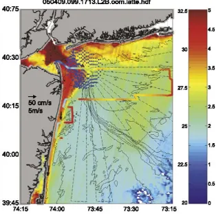
3.1 Hudson river outflow. The image was obtained from M ODIS at

17 : 13 GM T. Blue arrows show CODAR field, black arrows result from shelf moorings and white arrows fromN OAAmooring

at the Narrows. The color bar (right side) is for surface salinity

from the shiptrack shown in the figure (from Chant et al. (2008)). 12

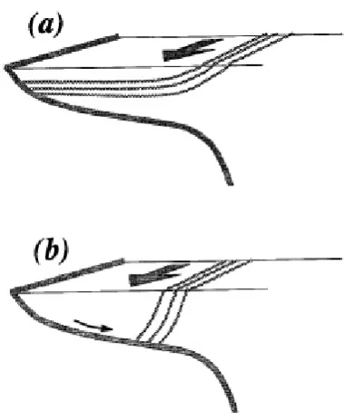
3.2 Sketches depicting (a) a surface-advected plume and (b) a

bottom-trapped plume. The large arrows indicate the direction of the

coastal plumes and the small arrow represents offshore transport

in the bottom Ekman layer (from Chapman & Lentz (1994)). . . . 15

3.3 Advanced very high resolution radiometer (AV HRR) IR image

on 22 July 1980, showing a series of well-developed cyclonic and anticyclonic eddies∼50 km in diameter. In both figures, A stands for Algiers. The eddies are underlined and labelled in the bottom

view to show that, going eastward, the cyclones (C) decrease while

the anticyclones (A) increase (From Millot (1985)). . . 17

(from Thomas & Linden (2007)). . . 20 4.2 Schematic of the view, along the across-shore direction, of a coastal

current flowing over an inclined wall in the laboratory. . . 23

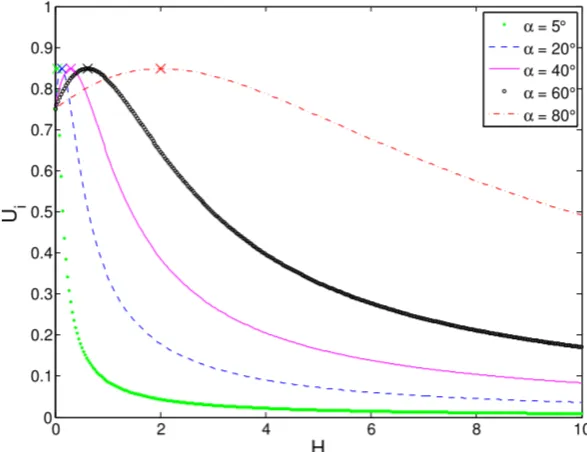
4.3 Variations of the non-dimensional theoretical inclined-wall coastal

current velocity,Ui, as a function of the bottom slope, α, and, the

non-dimensional height, H. . . 31

4.4 Variations of Ui, as a function of (a) Ω, for different values of α,

withq0 = 20cm3 s−1 andg0= 5cm s−2,(b)q0, for different values

of α, with Ω = 1.5rad s−1 and g0= 5 cm s−2, (c) g0, for different values of α, with Ω = 0.5 rad s−1 and q0 = 20 cm3 s−1. Crosses

indicate the maxima ofUi, found at (a) Ω = (tan(α))4/5g03/5_/4q1/5 0 ,

(b) q0 = (tan(α))4g03/210Ω5, (c) g0= 210/3Ω5/3q 1/3

0 /(tan(α))4/3. . . 34

4.5 Variations of the ratio,ui/u0, of the predicted inclined-wall coastal

current speed to the predicted vertical-wall coastal current speed

as a function of the bottom slope, α, and, the non-dimensional

height, H. . . 37

4.6 Variations of ui/u0 as a function of (a) Ω, for different values of

α, with q0 = 20 cm3 s−1 and g0 = 5 cm s−2,(b) q0, for

differ-ent values of α, with Ω = 1.5 rad s−1 and g0 = 5 cm s−2, (c) g0, for different values of α, with Ω = 0.5 rad s−1 and q0 =

20 cm3 _s−1_{. Crosses indicate the maxima of u}

i/u0, found at

(a) Ω = (tan(α))4/5_g03/5_/4q1/5

0 , (b) q0 = (tan(α))4g03/210Ω5, (c) g0= 210/3_Ω5/3_q1/3

0 /(tan(α))4/3. . . 38

5.1 Small-scale turntable at theFluid Dynamics Research Center

(Uni-versity of Warwick). . . 41

5.2 The two inclined walls for the small-scale experimental study . . . 42

5.3 Side-view video camera for capturing the coastal current height

profile. . . 44

5.4 P IV setup. . . 46 5.5 Results of the spatial and time averages on a single along-shore

velocity profile extracted from the P IV experiment J07 at the

fixed distance,dS, downstream from the source withdS = 77.5cm.

The colour bar on the figures is for velocity (cm s−1_{). . . . 49}

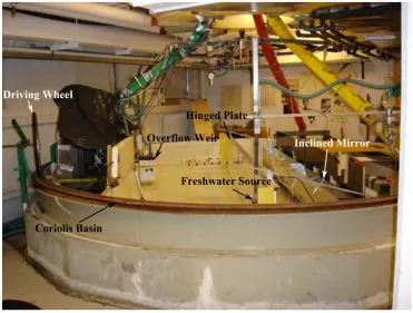
5.7 Picture of the Coriolis basin. . . 51

5.8 A cross-section of the 5 m diameter rotating turntable at the N T N U in Trondheim (from Vinger & McClimans (1980)). . . 52

5.9 Turntable drive mechanism. . . 52

5.10 Rotameter for measuring the flow rate, q0, at the source. . . 53

5.11 Freshwater Source. . . 54

5.12 Illustration of the method to measure the coastal current depth. . 55

5.13 Camera recording the coastal current depth. . . 55

6.1 ROM S configuration. . . 59

6.2 The different steps to find the flow rate in theROM S simulations; the figures display results for one specific run (plume 153, Table 7.1). 62 7.1 Top view of a coastal current simulated, (a) in the laboratory, (b) numerically. The images are taken at T=30. I = 0.301 ± 0.026, EkV = (1.4±0.3)×10−3, ROM S: EkH = 0, Laboratory experiment: EkH = 2.68 × 10−4. In (b), the color bar is for density(in kg m−3_{). . . . 68}

7.2 Nose propagation of the inviscid plumes. . . 70

7.3 Nose propagation of the viscous plumes. . . 71

7.4 Comparison of the non-dimensional plume length,L, as a function of the non-dimensional time, T, for inviscid and viscous numer-ical simulations, and laboratory experiments of Thomas & Lin-den (2007). The solid line represents the theoretical prediction, L= (3/4)T. . . 73

7.5 Summary of the non-dimensional plume width, W, as a function of the dimensionless time, T, for (a) all the inviscid numerical sim-ulations and (b) all the viscous numerical simsim-ulations. The width was measured at the non-dimensional distance, DS, downstream from the source, with DS = 12. The black curve on the figures of equation 0.2(T)12 is just to show that plume widths grow as T 1 2. . 75

7.6 Summary of the non-dimensional plume width,W, as a function of the dimensionless time, T, for theP IV vertical-wall experiments. The width was measured at the distance, dS, downstream from the source, with dS = 57.8 cm. The black curve on the figure of equation 0.2(T)12 is just to show that plume widths grow as T 1 2. . 76

simulation, one viscous numerical simulation and one laboratory experiments. The width was measured at the non-dimensional

dis-tance, DS, downstream from the source, with (a) DS = 28.8 and

(b) DS = 10. . . 77

7.8 Summary of the (averaged) non-dimensional plume width,W, as a

function of (a) the dimensionless parameter,I, and (b) the

horizon-tal Ekman number,EkH, respectively, for the viscous and inviscid

numerical simulations, and for the P IV laboratory experiments.

The black line on the figures identifies W = 1, that is agreement

between experiments and theory. The error bars are standard

de-viation errors of the averaged non-dimensional plume width. . . . 79 7.9 Summary of the maximum non-dimensional plume speed, Umax,

as a function of the dimensionless time, T, for (a) all the inviscid

numerical simulations and (b) all the viscous numerical

simula-tions. Umax was measured at the non-dimensional distance, DS,

downstream from the source, with DS = 12. The black line on

the Figure 7.9b identifies Umax = 1, that is agreement between

experiments and theory. . . 81

7.10 Summary of the maximum non-dimensional plume speed,Umax, as

a function of the dimensionless time, T, for theP IV vertical-wall experiments. Umax was measured at the distance,dS, downstream

from the source, with dS = 57.8 cm. The black line on the figures

identifies Umax = 1, that is agreement between experiments and

theory. . . 82

7.11 Maximum non-dimensional plume speed,Umax, as a function of the

dimensionless time, T, measured at the non-dimensional distance,

DS, downstream from the source, with DS = 10, for one inviscid

simulation, one viscous simulation and one laboratory experiment.

Umax was measured at the surface for the laboratory experiment and the viscous simulation, and, at the surface (N = 60) and

around 9 mm below the surface (N = 56) for the inviscid

simu-lation. I = 0.126±0.03, EkV = (5.73±1.79) ×10−3, Inviscid simulation: EkH = 0, Viscous simulation and laboratory

experi-ment: EkH = (1.26±0.29)×10−4. . . 83

the horizontal Ekman number, EkH, respectively, for the viscous and inviscid numerical simulations, and for the P IV laboratory

experiments. The black line on the figures identifies Umax = 1,

that is agreement between experiments and theory. The error

bars are standard deviation errors of the averaged maximum

non-dimensional plume speed. . . 85

7.13 Surface density field showing the unstable plumes (a) 148 and (b)

151 from the viscous numerical simulations. Color bar is for

den-sity (inkg m−3). . . 87

7.14 I-EkH diagram displaying the parametric locations where the plumes

are found to be stable/unstable. The dashed line is suggestive of the stability boundary. . . 88

8.1 Cross-section in they-zplane of (a)-(c) the non-dimensional

Corio-lis term in thev-momentum equation, and (b)-(d) the non-dimensional

pressure gradient term in thev-momentum equation, taken at the

alongshore distance upstream from the nose, dN = 5 cm, and at

the times (a)-(b)t = 4.25s and (c)-(d)t = 36.25s for the viscous

plume 150. . . 91

8.2 Cross-section in they-z plane of (a)-(c) the non-dimensional

along-shore velocity,U, for the inviscid plume 134 and the viscous plume 150, respectively, and (c)-(d) the density field for the inviscid

plume 134 and the viscous plume 150, respectively, taken at the

alongshore distance upstream from the nose, dN = 5 cm, and at

the time, t = 4.25 s. The color bar in the right images is for

density (in kg m−3_{). . . . . 92}

8.3 Cross-section in they-z plane of (a)-(c) the non-dimensional

along-shore velocity,U, for the inviscid plume 125 and the viscous plume

151, respectively, and (c)-(d) the density field for the inviscid

plume 125 and the viscous plume 151, respectively, taken at the alongshore distance upstream from the nose, dN = 5 cm, and at

the time, t = 4s. The color bar in the right images is for density

(in kg m−3_{). . . . 93}

150, respectively, and (c)-(d) the density field for the inviscid plume 134 and the viscous plume 150, respectively, taken at the

alongshore distance upstream from the nose, dN = 5 cm, and at

the time, t = 36.25 s. The color bar in the right images is for

density (in kg m−3_{). . . . . 95}

8.5 Cross-section in they-z plane of (a)-(c) the non-dimensional

along-shore velocity,U, for the viscous plumes 150 and 151, respectively,

and (c)-(d) the density field for the viscous plumes 150 and 151,

respectively, taken at the alongshore distance upstream from the

nose, dN = 50 cm, and at the time,t= 36 s. The color bar in the

right images is for density (inkg m−3). . . 96 8.6 Variations along the radial position of (a) the alongshore velocity,

u, (b) the across-shore velocity, v, and (c) the vertical velocity,

w, taken at the free surface, at different alongshore distances

up-stream from the plume nose,dN, and at the time,t= 40s, for the

inviscid plume 134. . . 98

8.7 Variations along the radial position of (a) the alongshore velocity,

u, (b) the across-shore velocity, v, and (c) the vertical velocity,

w, taken at the free surface, at different alongshore distances

up-stream from the plume nose,dN, and at the time,t= 40s, for the viscous plume 150. . . 99

8.8 Cross-section in thex-z plane of the density field taken at 4.8mm

from the wall and at the time t= 50 s for the inviscid plume 134

and the viscous plume 150, respectively. . . 100

8.9 Non-dimensional volume, Vi, of intermediate water in the coastal

plume and bulge system, as a function of (a) the dimensionless

time, T, and (b) the non-dimensional plume length, L, for the

inviscid and viscous numerical simulations. . . 101

8.10 Difference between the non-dimensional plume length, L, for the viscous simulations, and the theory of Thomas & Linden (2007),

L= (3/4)T. . . 103

(EkH)0.46. The velocity deficits are simply the slope of the best linear fits for the curves of Figure 8.10 computed from T ≥50. . . 104 9.1 A typical coastal current (experiment T35) flowing along an

in-clined plate mounted across the diameter of the Coriolis tank at

Trondheim. α = 50◦, I = 0.292, EkV = 6.6 ×10−4, EkH = 1.21×10−4_{, h}

0/HD = 0.49. . . 107 9.2 An unstable coastal current (experiment T32) flowing along an

inclined wall in the large-scale Coriolis tank at Trondheim. α =

50◦, I = 0.481, EkV = 2.43×10−4, EkH = 1.56×10−4,h0/HD = 0.92. . . 108

9.3 Comparison of the non-dimensional plume length, Li, as a func-tion of the dimensionless time,T, for small-scale experiments with

different sloping angles,α. . . 110

9.4 Comparison of the non-dimensional plume length, Li, as a

func-tion of the dimensionless time,T, for large-scale experiments with

different sloping angles,α. . . 111

9.5 Comparison of the non-dimensional plume length,Li, as a function

of the non-dimensional time, T, for small-scale experiments with

different sloping angles,α. The solid lines represent the theoretical

predictions for the different sloping angles according to (4.43). . . 113 9.6 Comparison of the non-dimensional plume length,Li, as a function

of the non-dimensional time, T, for large-scale experiments with

different sloping angles,α. The solid lines represent the theoretical

predictions for the different sloping angles according to (4.43). . . 114

9.7 Non-dimensional measured mean inclined-wall velocity,U_iexp, as a

function of the non-dimensional theoretical inclined-wall velocity,

U_ith, for the small-scale and large-scale inclined-wall experiments.

The solid line identifiesU_iexp =U_ith, while the dashed line identifies

the best linear fit given by 0.62U_ith+ 0.51 with a correlation of 0.21.116

speed, U_ith, as a function of (a) the dimensionless parameter, I, (b) the non-dimensional ambient depth parameter,h0/HD, for the

small-scale and large-scale inclined-wall experiments. The solid

line on each figure identifiesU_iexp =Uth

i . . . 118 9.9 Difference between the non-dimensional measured mean

inclined-wall speed, U_iexp, and the non-dimensional predicted inclined-wall

speed, Uth

i , as a function of (a) the horizontal Ekman number, EkH, (b) the vertical Ekman number, EkV, for the small-scale

and large-scale inclined-wall experiments. The solid line on each

figure identifiesU_iexp =U_ith. . . 119

9.10 Velocity deficit for the small-scale and large-scale inclined-wall ex-periments as a function of the horizontal Ekman number, EkH. . 120

9.11 Non-dimensional measured mean inclined-wall speed, U_iexp, as a

function of the horizontal Ekman number,EkH, for the small-scale

and large-scale inclined-wall experiments . . . 122

9.12 Non-dimensional measured mean inclined-wall velocity, (U_iexp)wi,

as a function of the non-dimensional theoretical inclined-wall

ve-locity, (U_ith)wi, for the small-scale and large-scale inclined-wall

ex-periments. The solid line identifies (U_iexp)wi = (U

th

i )wi, while the

dashed line identifies the best linear fit given by 1.19 (U_ith)wi+ 0.08

with a correlation of 0.64. . . 122

9.13 Non-dimensional measured mean inclined-wall speed, (U_iexp)wi, as

a function of (a) the dimensionless parameter, I, (b) the

non-dimensional ambient depth parameter, h0/HD, for the small-scale

and large-scale inclined-wall experiments. . . 124

9.14 Sketch from Thomas & Linden (2007) illustrating a side-view of a

plume. . . 125

9.15 Maximum measured plume height, him, near the source, as a

func-tion of the theoretical heights, h0 and hi, for vertical-wall and

inclined-wall plumes, respectively. The solid line identifies

agree-ment between the experiagree-ments and the theories, while the blue and

red dashed lines identify the best linear fits given by 0.91h0+ 2.52

with a correlation of 0.88, and 1.51 hi+ 0.7 with a correlation of

0.8, respectively. . . 126

inclined-wall experiments. The solid line represents the theoretical prediction, H = 2I5/4_{, while the dashed line is the best fit line}

given by 2.22(I)1.15_{. . . 127}

9.17 Summary of the non-dimensional plume width, Wi, as a function

of the dimensionless time, T, for theP IV small-scale vertical-wall

and inclined-wall experiments. The width was measured at the

distance, dS, downstream from the source, with dS = 57.8 cm.

The black curve on the figure of equation 0.2(T)12 is just to show

that the majority of the plume widths grows asT12. . . 128

9.18 Comparison of the non-dimensional plume width, Wi, as a

func-tion of the non-dimensional time, T, for P IV experiments with different sloping angles,α. . . 130

9.19 Summary of the (averaged) non-dimensional plume width, Wi, as

a function of H/tan(α) for the P IV small-scale inclined-wall

ex-periments. The solid line represents the theoretical prediction,

Wi =

p

(H/tan(α))2_{+ 1. The error bars are standard deviation}

errors of the averaged non-dimensional plume width. . . 131

9.20 Summary of the (averaged) non-dimensional plume width, Wi,

as a function of the non-dimensional ambient depth parameter,

h0/HD, for theP IV small-scale vertical-wall and inclined-wall

ex-periments. The error bars are standard deviation errors of the

averaged non-dimensional plume width. . . 131

9.21 Summary of the non-dimensional plume width, (Wi)wi, as a

func-tion of the dimensionless time, T, for theP IV small-scale

vertical-wall and inclined-vertical-wall experiments. The width was measured at

the distance,dS, downstream from the source, withdS = 57.8cm.

The black curve on the figure of equation 0.2(T)12 is just to show

that the majority of the plume widths grows asT12. . . 132

ter, h0/HD, and (b) the horizontal Ekman number, EkH,

respec-tively, for the P IV small-scale vertical-wall and inclined-wall

ex-periments. The solid line on the figures identifies (Wi)wi = 1, that

is agreement between experiments and theory. The error bars are

standard deviation errors of the averaged non-dimensional plume

width. . . 134

10.1 Schematic depicting the experimental configuration of Avicola &

Huq (2002) using the sloping bottom tank (from Avicola & Huq

(2002)). . . 137

10.2 Non-dimensional measured mean inclined-wall velocity, U_iexp, as a

function of the non-dimensional theoretical inclined-wall velocity,

Uth

i , for the experiments of Avicola & Huq (2002), Lentz & Helfrich (2002) and Whitehead & Chapman (1986). The solid line identifies

U_iexp =Uth

i , while the dashed line identifies the best linear fit given by 0.95Uth

i + 0.04 with a correlation of 0.86. . . 139 10.3 Ratio, U_iexp/U0, of the non-dimensional measured mean

inclined-wall velocity to the non-dimensional theoretical vertical-inclined-wall

ve-locity, as a function of H/tan(α), for the experiments of Avicola

& Huq (2002), Lentz & Helfrich (2002) and Whitehead &

Chap-man (1986). The solid line represents the theoretical prediction according to (4.65). . . 140

10.4 Non-dimensional measured mean inclined-wall velocity, (U_iexp)wi,

as a function of the non-dimensional theoretical inclined-wall

ve-locity, (Uth

i )wi, for the experiments of Avicola & Huq (2002), Lentz

& Helfrich (2002) and Whitehead & Chapman (1986). The solid

line identifies (U_iexp)wi = (U

th

i )wi, while the dashed line identifies

the best linear fit given by 1.04 (U_ith)wi −0.005 with a correlation

of 0.98. . . 141

10.5 Non-dimensional measured mean inclined-wall speed, U_iexp, as a function of (a) the dimensionless parameter,I, (b) the non-dimensional

ambient depth parameter, h0/HD, for the experiments of Avicola

& Huq (2002), Lentz & Helfrich (2002) and Whitehead &

Chap-man (1986). . . 142

speed, U_ith, as a function of (a) the dimensionless parameter, I, (b) the non-dimensional ambient depth parameter,h0/HD, for the

large-scale and small-scale experiments of this study, and for the

experiments of Avicola & Huq (2002), Lentz & Helfrich (2002)

and Whitehead & Chapman (1986). The solid line on each figure

identifies U_iexp =Uth

i . . . 144 10.7 Difference between the non-dimensional measured mean

inclined-wall speed, U_iexp, and the non-dimensional predicted inclined-wall

speed, U_ith, as a function of (a) the horizontal Ekman number,

EkH, (b) the vertical Ekman number, EkV, for the large-scale and

small-scale experiments of this study, and for the experiments of Avicola & Huq (2002), Lentz & Helfrich (2002) and Whitehead &

Chapman (1986). The solid line on each figure identifiesU_iexp =Uth i .145 10.8 (h0/HD)-EkH diagram displaying the parametric locations where

the plumes are found to be faster/slower than the theory, or to

have same speed than the theory. . . 146

10.9 Non-dimensional measured mean inclined-wall speed, U_iexp, as a

function of the horizontal Ekman number,EkH, for the large-scale

and small-scale experiments of this study and for the experiments

of Avicola & Huq (2002), Lentz & Helfrich (2002) and Whitehead & Chapman (1986). . . 147

10.10Measured inclined-wall width, w_iexp, as a function of the

theoreti-cal inclined-wall width,wth

i , for theP IV small-scale inclined-wall experiments and for the experiments of Avicola & Huq (2002) and

Lentz & Helfrich (2002). The solid line identifiesw_iexp =wth i , while the dashed line identifies the best linear fit given by 0.95wth

i + 3.16 with a correlation of 0.9. . . 148

10.11Summary of the non-dimensional plume width, Wi, as a function

of the non-dimensional ambient depth parameter, h0/HD, for the P IV small-scale inclined-wall experiments and for the experiments

of Avicola & Huq (2002) and Lentz & Helfrich (2002). . . 149

and (b) the horizontal Ekman number, EkH, respectively, for the P IV small-scale vertical-wall and inclined-wall experiments and

for the experiments of Avicola & Huq (2002) and Lentz & Helfrich

(2002). The solid line on the figures identifies (Wi)wi = 1, that is

agreement between experiments and theory. . . 150

10.13Measured mean inclined-wall speed, uexp_i , as a function of (a) the

theoretical inclined-wall speed, uth

i , defined in (4.42), and (b) the theoretical inclined-wall speed, cp, of Lentz & Helfrich (2002), for

the small-scale experiments of this study and for the experiments

of Avicola & Huq (2002), Lentz & Helfrich (2002) and Whitehead

& Chapman (1986). The solid line in the figures identifies (a)

uexp_i = uth

i and (b) u exp

i = cp, while the dashed line identifies the best linear fit given by (a) 0.89uth

i + 0.08 with a correlation of 0.75 and (b)0.65cp+ 0.52 with a correlation of 0.66. . . 153

10.14Measured mean inclined-wall speed, uexp_i , as a function of (a) the

theoretical inclined-wall speed, uth

i , defined in (4.42), and (b) the theoretical inclined-wall speed, cp, of Lentz & Helfrich (2002), for

the large-scale experiments of this study. The solid line in the

figures identifies (a)uexp_i =uth_i and (b)uexp_i =cp, while the dashed

line identifies the best linear fit given by (a) 1.65uth_i + 0.35 with a correlation of 0.73 and (b)1.17cp+ 2.13 with a correlation of 0.63.154

10.15Measured inclined-wall width,w_iexp, as a function of the theoretical

inclined-wall width, wp, of Lentz & Helfrich (2002), for the P IV

small-scale inclined-wall experiments and for the experiments of

Avicola & Huq (2002) and Lentz & Helfrich (2002). The solid line

identifieswexp_i =wp, while the dashed line identifies the best linear

fit given by 0.94 wp+ 1.93 with a correlation of 0.9. . . 155

10.16Summary of the non-dimensional plume width, (Wi)wp, as a

func-tion of (a) the non-dimensional ambient depth parameter,h0/HD,

and (b) the horizontal Ekman number, EkH, for the P IV

small-scale vertical-wall and inclined-wall experiments and for the

exper-iments of Avicola & Huq (2002) and Lentz & Helfrich (2002). The

solid line on the figures identifies (Wi)wp = 1, that is agreement

between experiments and theory. . . 156

i

theoretical inclined-wall speed, cp, of Lentz & Helfrich (2002), for the plumes tabulated in Table 10.1. The solid line in the figures

identifies (a)uf ield_i =uth

i and (b) u f ield

i =cp, while the dashed line identifies the best linear fit given by (a) 1.04 uth

i + 0.06 with a correlation of 0.79 and (b)0.48cp+ 0.25 with a correlation of 0.55. 159

10.18Ratio, U_if ield/U0, of the non-dimensional observed alongshore

ve-locity to the non-dimensional theoretical vertical-wall veve-locity, as

a function of H/tan(α), for the plumes tabulated in Table 10.1.

The solid line represents the theoretical prediction according to

(4.65). . . 160

10.19Observed width,wf ield_i , as a function of (a) the theoretical inclined-wall width,wth

i , defined in (4.36), and (b) the theoretical inclined-wall width, wp, of Lentz & Helfrich (2002), for the plumes

tab-ulated in Table 10.1. The solid line in the figures identifies (a)

w_if ield = wth

i and (b) w f ield

i = wp, while the dashed line identifies the best linear fit given by (a) 0.85 wth

i + 6009 with a correlation of 0.67 and (b)0.54wp+ 11690 with a correlation of 0.55. . . 161

11.1 Non-dimensional current length,L, as a function of the

dimension-less time, T,for three small-scale vertical-wall experiments with

different ambient ocean depth,HD. . . 163 11.2 Non-dimensional current length,L, as a function of the

dimension-less time, T, for the surface-advected plumes from the small-scale

experiments of Thomas & Linden (2007). . . 164

11.3 Non-dimensional current length, L, as a function of the

dimen-sionless time, T, for the surface-advected plumes from the

small-scale inclined-wall experiments presented in this study and for the

bottom-trapped experiment, F, of Avicola & Huq (2002). . . 165

11.4 Alongshore velocity, u (cm s−1), as a function of the time, t (s),

measured at the alongshore distance downstream from the source, ds = 112.4 cm, for twoP IV vertical-wall experiments with

differ-ent ambidiffer-ent ocean depth, HD. The color bar in each figure is for

velocity (in cm s−1_{). . . 166}

depth,HD, measured at the alongshore distance downstream from the source, ds= 112.4 cm, and at the timet = 124.48s. . . 167

Introduction & Problem

Introduction

An important objective in physical oceanography is to understand the dynamics

of buoyant discharge and mixing in the coastal ocean. The oceans and coastal

areas of the Earth are indeed complex and dynamic natural systems. Pollution

and human effects can impact these delicate ecosystems drastically.

Buoyant fluid entering the coastal ocean from, for example, an estuary will

typically form a gravity-driven surface flow. The flow develops as a consequence of the density difference between the discharged, buoyant freshwater and the

denser, more saline ocean water. Such flows are a major source of nutrients,

sed-iments and contaminants to coastal waters, and may help to support diverse and

productive ecosystems. These flows often play an important role in enabling the

exchange of water between coastal channels and the open sea. When the

buoy-ant outflow exceeds length scales larger than the Rossby deformation scale, its

dynamics is affected by the Coriolis force arising from the rotation of the Earth.

As a result, the discharged fresh water is confined to the coastal zone where it

forms a current flowing along the coast in the direction of Kelvin wave prop-agation. This study concentrates on examining the dynamics and evolution of

gravity-driven coastal currents flowing along a simple vertical-wall coastline, and

along a more realistic coastline topography as represented by inclined coastlines.

Firstly, laboratory studies for gravity-driven coastal currents flowing along

a vertical-wall coastline (those of Thomas & Linden (2007) and additional

ex-periments performed at Warwick University) are combined with numerical

sim-ulations employing the Regional Ocean Modeling System (ROM S) to further

investigate departures from the geostrophic theory of Thomas & Linden (2007).

A particular attention is paid to the internal dynamics of the plumes, the occur-rence of instabilities within them, and the role of viscous forces in their evolution.

Secondly, the geostrophic model of Thomas & Linden (2007) for gravity-driven

coastal currents flowing along vertical-wall coastlines is extended to the more

realistic case of inclined coastlines. The prediction of the extended model is com-pared to two new laboratory studies for coastal currents flowing along inclined

coastlines and to the experimental studies of Avicola & Huq (2002), Whitehead &

Chapman (1986) and Lentz & Helfrich (2002) who also carried out experiments

for coastal currents flowing along sloping walls. The extended model and the

five experimental studies are as well compared to the scaling theory of Lentz &

Helfrich (2002) for inclined-wall coastal currents. Both, the extended geostrophic

model and the scaling theory of Lentz & Helfrich (2002), are finally compared

to oceanic observations. Lastly, a small set of laboratory experiments for coastal

currents flowing along vertical-wall coastlines when decreasing the ambient ocean

depth is examined.

The plan of this thesis is as follows. In the first part of this thesis, the

gen-eral background on gravity-driven coastal currents, some previous numerical and

experimental studies, and the methods (theoretical, experimental, numerical)

em-ployed here are reviewed. The second part uses the vertical-wall laboratory and

numerical studies together to explore the kinematic properties of the

buoyancy-driven plumes, and to identify their non-dimensional dependencies. The internal

dynamics of the plumes are also investigated. The third part presents the

re-sults of the two new inclined-wall laboratory studies and compared them to the

extended geostrophic model, the experimental studies of Avicola & Huq (2002), Whitehead & Chapman (1986) and Lentz & Helfrich (2002), and the scaling

the-ory of Lentz & Helfrich (2002). The extended geostrophic model and the scaling

theory of Lentz & Helfrich (2002) are compared as well to oceanic observations.

The results of the study for vertical-wall coastal currents when decreasing the

ambient ocean depth are lastly explored. A final part offers a summary and

General background

A gravity current, also called density current or buoyancy current, is the flow

of one fluid within another caused by the density difference between the fluids.

The density difference between two fluids, or between different parts of the same

fluid, can exist because of a difference in temperature, salinity, or concentration

of suspended sediment. It is characterised by the reduced gravity∗,g0, defined by

g0 = ρ2−ρ1

ρ1

g, (2.1)

where ρ1 and ρ2 are the densities of the two fluids and g = 981 cm s−2 is the

acceleration due to gravity. Gravity currents are primarily horizontal, occurring

as either top or bottom boundary currents, or as intrusions at some intermediate

level, and are associated with strong density fronts. On the ocean surface, the

front of a gravity current sometimes forms a colour change in the water, but more often can be seen from foam and floating debris which collect along the line of

converging flow. These fronts may have multiple lines, as shown in Figure 2.1

taken at Trondheim in Norway.

Much of the dynamics of gravity currents has been discovered from laboratory

experiments in which salt water was released from behind a lock gate into a

large tank of freshwater. Figure 2.2 is a photograph of this type of laboratory

experiment from Simpson & Britter (1979), using shadowgraphy, which displays

the side view of a gravity current moving from left to right in lock-exchange flow.

The structure of the leading front in Figure 2.2 is typical of the structure of a gravity current. There is a raised part, which is called the head, and a following

shallower part, called the tail. In the tail and in the ambient fluid ahead, the

∗ _{The reduced gravity represents the effective change in the acceleration of gravity acting}

on one fluid in contact with a fluid of different density due to buoyancy forces.

Figure 2.1: Foam fronts observed in the Flakk Fjord at Trondheim in Norway (from Ellingsen (2004)).

Ambient freshwater

Head of the gravity current Tail of the gravity

current

Gravity current of salt water

pressure is hydrostatic. At the head the ambient fluid is displaced upwards over

the gravity current; consequently, the pressure there is not hydrostatic. The

main transfer of momentum (between the gravity current and the ambient fluid) occurs at the head, and so this is the most dynamically significant part of the

flow. Indeed, the formation of the ”head” may be considered to be the fluid’s

response to the imposed difference in hydrostatic pressure (Hacker (1996)).

There are many examples of gravity currents occurring in the environment,

which are discussed in Simpson (1987). One particular example of gravity

cur-rents produced by direct inputs of buoyancy, and of particular interest for this

thesis, is in the estuarine environment, where the freshwater from a river meets

the saltier sea water.

2.1

Coriolis effects on gravity currents

When gravity currents occur on length and time scales which are sufficiently large,

their dynamics are influenced by the rotation of the Earth and they undergo a

Coriolis force,FC =−2Ω×u, whereurepresents the velocity vector of a gravity

current fluid particle, and Ωis the angular velocity vector of the Earth, pointing out of the ground in the northern hemisphere. The Earth is taken as a perfect

sphere. This sphere rotates about its North Pole-South Pole axis. At any given

latitude ϕ, the north-south direction departs from the local vertical. Figure 2.3 depicts the traditional choice for a local Cartesian framework of reference: the

x-axis is oriented eastward, the y-axis, northward, and the z-axis, upward. The

corresponding unit vectors are denoted (i,j,k). In this framework, the Coriolis

force is expressed as

FC = (−f∗w+f v)i−f uj+f∗uk, (2.2)

where u, v and w are the components of the velocity vector u in the x-, y- and

z-directions, respectively, and f = 2Ω sinϕ is the Coriolis parameter, whereas

f∗ = 2Ω cosϕ is the reciprocal Coriolis parameter. In the northern hemisphere,

f is positive; it is zero at the equator and negative in the southern hemisphere. In contrast, f∗ is positive in both hemispheres, but it vanishes at the poles.

Generally, the f-terms are important, whereas the f∗-terms can be neglected

(Cushman-Roisin (1994)). Thus in the preceding framework, the Coriolis force

Figure 2.3: Definition of a local Cartesian framework of reference on a spherical Earth. The coordinate x is directed eastward,y northward, and z upward (from Cushman-Roisin (1994)).

FC =f vi−f uj. (2.3)

In the absence of boundaries, a gravity current is deflected from its initial

course by the Coriolis force, to the right in the northern hemisphere, and to the

left in the southern hemisphere and is constrained to form an eddy. A stationary

equilibrium may be reached in which Coriolis forces balance the radial pressure

gradient†. This is called geostrophic balance, the circulating region of the gravity

current is called a geostrophic eddy. Further release of potential energy is only

possible through instability processes or through viscous dissipation (Griffiths

(1986) and Hacker (1996)). The familiar ”highs” and ”lows” of weather maps

are examples of geostrophic eddies in the atmosphere; similar flows occur in the oceans (although on a smaller scale) and are called mesoscale eddies. The process

described above through which a geostrophic flow may be established, is called

Rossby or ”geostrophic” adjustment (Rossby (1938)).

In the vicinity of a boundary, velocities normal to the boundary, and hence

Coriolis forces parallel to the boundary, must vanish. The constraints of the

rotation are broken, and a gravity current flows along the boundary (Griffiths

†_{This is strictly the case if the radius of curvature of the region of the gravity current is}

(1986)). Boundaries may be mountain ranges, coastlines, or a sloping ocean

bottom. River outflows are localized sources of fresh, less dense water that (in

the absence of advecting currents) are confined by Coriolis forces to spread in only one direction along the coast. The coast may have any orientation, but the

gravity current must have the coast on its right-hand side when looking in the

direction of the flow in the northern hemisphere, or on its left in the southern

hemisphere. When the gravity current is stable, the flow approaches a state of

geostrophic equilibrium and the interface at the edge of the region of fresh fluid

slopes in order to provide a hydrostatic pressure gradient to balance the Coriolis

force exerted on the flow.

2.2

Potential vorticity

The Rossby adjustment process may also be understood in terms of the

conser-vation of the potential vorticity (Hacker (1996)). In fluid dynamics, vorticity is

the curl of the fluid velocity. In the simplest sense, vorticity is the tendency for

elements of the fluid to ”spin”. More formally, vorticity can be related to the

amount of ”circulation” or ”rotation” (or more strictly, the local angular rate of rotation) in a fluid. In the study of geostrophic flows, since the horizontal

flow field has no depth-dependence, there is no vertical shear and no eddies with

horizontal axes (Cushman-Roisin (1994)). Thus, the absolute vorticity of a fluid

particle, for a geostrophic flow, is

f +ξ (2.4)

where f is the ambient vorticity and ξ = ∂v_∂x − ∂u

∂y is the relative vorticity of the fluid particle. The vorticity vector is strictly vertical, and the preceding

expression merely shows this vertical component. The potential vorticity,q, of a

fluid parcel is the ratio of its absolute vorticity to its height, h:

q= f+ξ

h . (2.5)

From the momentum and continuity equations of geostrophic flows, it can

be shown that, in the absence of dissipation, the fluid parcel’s volume and its

circulation are conserved, implying the conservation of their ratio defined as the

potential vorticity, q(Cushman-Roisin (1994)). Thus, the potential vorticity can

Figure 2.4: Conservation of volume and circulation of a fluid parcel undergo-ing squeezundergo-ing or stretchundergo-ing, implyundergo-ing conservation of potential vorticity (from Cushman-Roisin (1994).

The best example to explain this conservation principle is that of a ballerina

spinning on her toes; with her arms stretched out, she spins slowly, but with her

arms brought against her body, she spins more rapidly. Likewise in homogeneous

geophysical flows, when a parcel of fluid is squeezed laterally (its cross-sectional

area ds decreasing), its vorticity must increase (f +ϕ increasing) to conserve

circulation (see figure 2.4).

2.3

Governing non-dimensional parameters

The length scale RD, called the Rossby radius of deformation, and defined as

RD =

√

g0H

f , (2.6)

wheref is the Coriolis parameter, g0is defined in (2.1) and H is the height scale of the flow, is the fundamental length scale in all problems involving buoyancy

forces and background rotation, since it is the length scale over which a density

interface will slope in order to balance a buoyancy driven flow. In the Rossby

adjustment process,RD indicates the distance over which the fluid spreads before

balance between the pressure gradient and Coriolis forces is obtained. The width

of a gravity oceanic coastal current is expected to scale onRD.

The associated dimensionless number is the Rossby number, Ro, defined as

Ro= U

where U and L are, respectively, characteristic velocity and horizontal length

scales of the flow. Ro compares inertial to Coriolis forces and is fundamental

in geophysical fluid dynamics, where it characterizes the importance of Coriolis accelerations arising from planetary rotation. For a fluid system strongly affected

by Coriolis forces, Ro <<1.

The relative importance of friction is measured by the Ekman number, Ek,

which is the ratio of viscous to Coriolis forces. This number is defined as

Ek = ν

f D, (2.8)

whereνis the kinematic viscosity andDis a characteristic (horizontal or vertical)

length scale of the flow. It gives a measure at which stresses at a boundary

are communicated to the fluid interior. For geophysical flows, this number is exceedingly small; it is very small even in the laboratory.

The Reynolds number, Re, which compares inertial to viscous forces, is

de-fined as

Re= U D

ν . (2.9)

In most cases of geophysical interest, the Reynolds number is quite large. The

densimetric Froude number, F r, defined as

F r= √U

g0H, (2.10)

is a ratio of inertial to buoyancy forces. Finally, the Burger number, Bu, defined

as

Bu= (Ro

F r)

2_{, (2.11)}

indicates the importance of the stratification of the flow. This number is often

of order one for many atmospheric phenomena, meaning that both stratification

and rotation play nearly equal roles in governing vertical and other motions in

Overview of prior studies

Buoyant outflows occur commonly and have been studied in various localities

throughout the world. They can be formed from processes other than river

discharges: for example, outflows from oceanic straits in which there are

signifi-cant density differences can also form coastal currents. Many field investigations

have been carried out during the last century along coastlines throughout the

world to study the dynamics of these currents and understand the impacts they can have on near shore marine activities and biological population. Examples

of buoyancy-driven coastal currents include the Columbia River Plume (Hickey

et al. (1998)), the Delaware Coastal Current ((Munchow & Garvine, 1993a;b)),

the Hudson River outflow (Chant et al. (2008)) and the Algerian Current

(Oba-ton et al. (2000)), among others. The reader is referred to Chant (2011) for a

detailed review of the systems observed and their properties.

Garvine (1995) developed a classification of buoyant outflows as either

”small-scale” or ”large-”small-scale” dependent upon the cross-shore Kelvin number, K, the

ratio of the plume width to the baroclinic Rossby radius, RD. ”Small-scale” outflows, with Kelvin numbers less than 1, are those in which inertial effects are

greater than rotation, and outflows tend to spread laterally and to be trapped

by advection near the source. An example of this type of ”small-scale” outflow

is the Connecticut river plume (Garvine (1977)). ”Large-scale” outflows have a

Kelvin number on the order 1 or greater; such outflows are dominated by the

Earth’s rotation and form coastally trapped currents that flow in the direction

of Kelvin wave propagation. It is this latter category with which this study is

concerned. Figure 3.1, from Chant et al. (2008), illustrates some of the observed

properties of ”large-scale”river plumes for the case of the Hudson River. Note in particular the presence of the bulge of buoyant water near the estuary mouth and

the narrow coastal current emanating from it. The coastal current flows in the

direction of Kelvin wave propagation, that is with the coast on its right (northern

hemisphere).

Figure 3.1: Hudson river outflow. The image was obtained from M ODIS at 17 : 13 GM T. Blue arrows show CODAR field, black arrows result from shelf moorings and white arrows from N OAA mooring at the Narrows. The color bar (right side) is for surface salinity from the shiptrack shown in the figure (from Chant et al. (2008)).

3.1

Prior studies on coastal current dynamics

The coastal current is the most common structure observed in field studies (e.g.

Figure 3.1). It is a region of downshelf transport of buoyant fluid (downshelf is

defined as the direction of Kelvin wave propagation). Previous laboratory and

Early laboratory experiments (e.g. Stern et al. (1982)) examined the

propa-gation of a coastal current formed from a dam-break. The study of Stern et al.

(1982) focused primarily on the geometry and propagation of the leading edge (nose) of the coastal current. Thomas & Linden (2007) investigated the

dynam-ics of a coastal current when the freshwater was discharged continuously from a

point source. In their experimental study, the width, the depth and the

propaga-tion speed of coastal currents moving along a vertical wall were determined. The

experimental data were compared to their theoretical model based on geostrophy,

continuity and conservation of potential vorticity (described in greater detail in

Chapter 4). Overall, good agreement between the experiments of Thomas &

Linden (2007) and their theory was obtained.

On the numerical side, many studies found that the coastal current was largely

in geostrophic equilibrium. Chao & Boicourt (1986) divided the plume into two dynamically distinct regions: a bulge region near the estuary mouth and a

downstream coastal current. They looked at the dynamics at the river mouth.

Chao & Boicourt (1986) found that the nose of the coastal current advances faster

in the estuary region than down the coast and suggested that mixing near the

estuary mouth was responsible for the coastal current slowing down.

Whitehead & Chapman (1986) conducted experiments of a coastal current

propagating along a vertical wall which ultimately encountered a sloping bottom

and continued to flow along the sloping wall. They observed that the sloping

bottom had a dynamically significant effect on the evolution of the coastal cur-rent: indeed coastal currents were seen to decelerate and widen in the region

of the sloping bottom. However, Whitehead & Chapman (1986) did not offer a

dynamical explanation for their results.

Attempts to classify the dynamics of coastal currents have been undertaken.

With their numerical study, Chao (1988) proposed a classification scheme based

upon an internal Froude number and a dissipation parameter. Csanady (1984)

and Wright (1989) simulated a surface-to-bottom density front (i.e. plumes from

which the buoyant water is in contact with the bottom, also referred to as

bottom-advected plumes (Figure 3.2(b))) over a sloping bottom and a flat continental shelf, respectively, and noted that offshore transport of buoyant water in the

bot-tom boundary layer contributed to the cross shelf movement of botbot-tom advected

plumes. Pursuing this result, Chapman & Lentz (1994) examined the role of

bottom friction on the development of a coastal current. They suggested that

Ekman layer may transport fluid offshore, and the coastal current may spread

offshore to the point at which the along-shore velocity, and therefore the bottom

Ekman layer flux, would decrease to zero.

Yankovsky & Chapman (1997) produced a scaling for a gravity current flowing

over a continental shelf which distinguishes a surface-advected gravity current

(Figure 3.2(a)), which is isolated from the bottom, with a bottom-trapped gravity

current (Figure 3.2(b)), for which the buoyant water is in contact with the bottom

and bottom friction is important in the establishment of the coastal current. They

showed that in equilibrium the depth where the front intersects the bottom is

the same depth as the depth for a gravity current flowing along a vertical wall.

However, Yankovsky & Chapman (1997) examined whether the structure of a

gravity current more closely resembles the surface-trapped or slope-controlled

case for the region near the source and not for the coastal current away from the source. To investigate this latter issue, Lentz & Helfrich (2002) proposed a

scaling theory for gravity currents flowing over a sloping bottom. Lentz & Helfrich

(2002) also simulated gravity currents flowing along an inclined coastline in the

laboratory : their experimental results were found to be consistent with their

scaling theory.

Avicola & Huq (2002) simulated in the laboratory surface-advected and

bottom-trapped plumes flowing over a continental shelf. They derived a theoretical model

based on the assumption that the frontal dynamics are those of a Margules front.

The theoretical expressions obtained by Avicola & Huq (2002) are similar to those obtained by Thomas & Linden (2007) (who assumed geostrophic

equilib-rium). Avicola & Huq (2002) classified the dynamics of coastal currents into

a two-variable non-dimensional parameter space comprising an ambient depth

parameter and a bottom slope parameter. Their resulting parameter space was

found to delineate surface-advected currents to bottom-trapped currents.

3.2

Prior studies on the bulge region

The recirculating bulge region can be described as a large (relative to the coastal

current width) freshwater lens rotating clockwise (in the northern hemisphere)

located downstream to the source region. These features are rarely seen in nature

(e.g. Figure 3.1), although they are quite common in numerical and laboratory

Figure 3.2: Sketches depicting (a) a surface-advected plume and (b) a bottom-trapped plume. The large arrows indicate the direction of the coastal plumes and the small arrow represents offshore transport in the bottom Ekman layer (from Chapman & Lentz (1994)).

Yankovsky & Chapman (1997) used a gradient wind balance∗ to predict the

maximum size of the recirculating bulge. They predicted a maximum

recirculat-ing bulge radius for surface-advected plumes. Nof & Pichevin (2001) analytically

hypothesized a mechanism for the bulge growth rate, based upon momentum

conservation arguments.

For his numerical simulations, Garvine (2001) noted that a buoyant outflow in deep water will form a recirculating bulge and a coastal current, while an

outflow in shallow water will form an upshelf intrusion and a coastal current.

Avicola & Huq (2003a) experimentally examined the growth and characteristics

of a recirculating bulge formed from a surface-advected plume exiting a strait or

an estuary. When recirculating bulges formed, Avicola & Huq (2003a) determined

that the freshwater storage within the bulge was approximately 60% to 70% of

the source freshwater flux. Similarly, Horner-Devine et al. (2006) found that

the growth of the bulge and the accumulation of fluid within it coincided with

a reduction in the coastal current transport to approximately 50% of the inflow

∗_{Gradient wind balance is a balance between Coriolis, centrifugal and pressure gradient}