Testing a technique to generate low frequency large scale turbulence with the Wall of Wind : an experimental study

Testing a technique to generate low-frequency

large-scale turbulence with the Wall of Wind

An experimental study

MSc Internship Report

Internship performed at the University of Auckland, New-Zealand, September-December 2013

Testing a technique to generate low-frequency large-scale

turbulence with the Wall of Wind: an experimental study

Author: Max Haspels

Preface

The goal of the internship, which is part of the Mechanical Engineering curriculum, is to let the student gain work experience in an industrial or research environment. The student gets an impression of working life and has to put his knowledge into practice. A lot of students use this opportunity to go abroad to gain experience in an international environment. With this in mind, I choose to go to New-Zealand and carry out my internship at the University of Auckland. During the months September and December 2013, I have been working on a research project which was supervised by associate professor Peter Richards. This report describes my research project, testing an experimental technique which could ultimately be used in the Wall of Wind. The Wall of Wind is a large experimental setup which is able to simulate hurricane winds, located at Florida International University.

I would like to thank my university supervisor, professor Harry Hoeijmakers of the Engineering Fluid Dynamics group for arranging my placement at the University of Auckland. The research project came from Peter Richards who will be spending five months in 2014 at Florida International University during his sabbatical, helping the Wall of Wind researchers. I would like to thank Peter for his help during my project and the good time I experienced at the University of Auckland.

Max Haspels

Contents

Preface i

1 Introduction 1

2 Wall of Wind 2

3 Problem definition 3

4 Silsoe Cube 4

5 Turbulence 5

5.1 Fourier analysis . . . 5 5.2 Turbulence spectra . . . 6 5.3 Analysing the spectra . . . 7

6 Concept 9

6.1 Literature . . . 9 6.2 First tests . . . 9 6.3 Concept test results . . . 10

7 Wall of Wind scale model 11

7.1 Scale model . . . 11 7.2 Approach . . . 12 7.3 Turbulence measurements . . . 12

8 Open-jet facility 16

8.1 Turbulence measurements . . . 16 8.2 Pressure measurements . . . 20

Conclusion 31

Bibliography I

A Spectral analysis Matlab script II

B Power spectra of the Spires configuration and the Vane configurations IV

1

Introduction

The Wall of Wind is a large experimental setup, which is capable of simulating hurricane winds, located at the Florida International University (FIU). One of the goals of the Wall of Wind is to enhance full scale testing to gain a better understanding of the interaction between hurricane winds and structures like residential buildings, without dealing with scaling issues. Turbulence is one of the most important features of hurricane winds as these flows cause unsteady loads on structures. To model proper hurricane winds, the Wall of Wind should be able to generate a flow with turbulent structures comparable to the turbulent structures in the atmospheric boundary layer (ABL). From February 2014, associate professor Peter Richards will spend 5 months in the United States to help the researchers of the International Hurricane Research Center (IHRC) with research on the WoW. One of the things he will consider is modeling low-frequency large-scale turbulence, the WoW is not yet capable of generating large-scale turbulent structures. A technique which possibly could be used to generate turbulence with the WoW is studied in this report.

2

Wall of Wind

Among all the natural disasters, hurricanes play major role in the insurance losses which are associated with damage on low-rise structures. Most of the damage caused by hurricanes is not associated with high-rise structures but rather with low-rise structures like residential or industrial buildings. The wind loading codes which are used in the design process of these buildings are mostly based on practice rather than on any form of technical research. In 2003 the research team of the IHRC of FIU started planning the construction of a large open-jet wind testing facility. Despite the possibilities of Computational Fluid Dynamics wind tunnel testing with scale models is still the most common tool in predicting wind loading. Aly et al. [2011] note: In addition to wind-tunnel tests, full-scale testing and measurement of wind effects play an important role and: To overcome scaling issues and enhance capabilities to conduct destructive testing under hurricane winds and rain, researchers at the Florida International University (FIU) have developed a new open jet facility, the Wall of Wind (WoW). The Wall of Wind is an open-loop wind tunnel which contains twelve fans which can produce a combined flow up to 1360m3_{/s at 8000bhp. The}

flow produced by the fans is forced into a contraction and enters the flow conditioning section. The flow conditioning section contains vertical spires at the inlet and roughness elements on the floor to generate turbulence and create the required velocity boundary layer. The WoW was designed to model the characteristics of the Atmospheric Boundary Layer (ABL) as most of the buildings are located in this bottommost layer of the atmosphere. The maximum wind speeds that can be achieved are in excess of 70m/sand the WoW is capable of generating the velocity profile of a category 5 hurricane. The WoW is currently in business and used for non-destructive and destructive testing.

(a) Fans (b) Schematic overview

3

Problem definition

To model the effects and the behaviour of hurricane winds there is more needed than just the generation of very high wind speeds. The unsteady behaviour of the flow is very important as unsteady loads created by turbulence can be more devastating than sustained loads. As it has hard for any test facility to fully reproduce all the features of the flow in the ABL, it must be investigated which are the most important features to model. One of the features noted on the FIU website is the holistic full- scale simulation of hurricane wind forces, turbulences and vortices. In 2014 associate professor Peter Richards will spend five months in Miami to assist the IHRC team with the development of equipment, testing techniques and analysis procedures. One of the aspects he will consider will be the generation of large-scale low-frequency fluctuations in the flow. These fluctuations can be considered as turbulent structures which totally engulf a structure and its associated local flow field. When these large-scale turbulent structures are not modeled properly the tests conducted with the Wall of Wind only apply to conditions that in reality last for a short duration.

Richards et al. [2007] use mean pressure coefficients reported by a German comparative study to show that mean pressure coefficients are sensitive to the intensities of high-frequency small-scale turbulence in the associated flow field. They also modeled the Silsoe Cube on a 1:40 scale in the wind tunnel of the University of Auckland and showed that mean pressures similar to the full scale situation can be obtained by matching the high-frequency end of the turbulence spectrum. It is demonstrated that a lack of low-frequency turbulence results in a reduced standard deviation of mean wind direction which mainly affects the observed maximum and minimum pressures. As these maximum and minimum pressures play a major role in damaging the structure, proper modeling of low-frequency turbulence is required for the Wall of Wind to be a valid test facility.

The goal of this research is to find and test a technique which can be used to model low-frequency large-scale turbulence with the Wall of Wind.

4

Silsoe Cube

The Silsoe Cube provides a facility for fundamental studies on the interaction between wind and a building. The Silsoe Cube is located at the Silsoe Research Institute in the UK. The 6mcube has a vertical and horizontal ring of pressure taps with additional taps on a quarter of the roof. The white spots in figure 4.1 mark the horizontal and vertical pressure taps. Richards et al. [2001] discuss the results of the flow of natural wind around a cube that include surface pressure measurements and velocity measurements, which is believed to be the first study ever on the subject. The results are compared with results from different wind tunnel tests and it is showed that there is certain agreement, but there are also differences in the observed pressures at certain pressure taps. The difference between the results of the wind tunnel tests and the Silsoe Cube measurements show that data from experiments with the full scale Silsoe Cube are very valuable for the field of wind engineering. More detailed results are provided by Richards and Hoxey [2012a], these results are very useful for comparison studies involving wind tunnel modeling of low-rise buildings or computational fluid dynamics.

Aly et al. [2011] discuss one of the final stages in the design process of the Wall of Wind. Using a scale model and computational fluid dynamics they determine the optimal scale of the test model and the ideal distance from the outlet of the WoW to the test model. The test model is a scale model of the Silsoe Cube and the observed pressures are compared to the full scale Silsoe Cube data. More recent pressure measurements which were done during experiments with the full scale WoW also used a scale model of the Silsoe Cube. At the University of Auckland there is a 1:40 scale model of the Silsoe Cube available which was used in experiments discussed by Richards et al. [2007]. As the data obtained by experiments with the full scale Silsoe Cube is used as reference data in previous research on the WoW and there is already a scale model available, the full scale Silsoe data is also used as reference data in this study.

5

Turbulence

Turbulent flow is a flow regime which is highly irregular and is characterized by changing properties as pressure and velocity in space and time. The properties of turbulent flow which are of interest in this study are the variations in the flow velocity and the associated pressure fluctuations on structures. If we want to analyse a velocity history record of a turbulent flow on a certain time interval it does not make sense to analyse the velocity history in the time domain. Figure 5.1 shows the time history record of the velocity of a turbulent flow. The velocity fluctuations seem to be random and the graph is not very useful for further analysis. But if we divide the velocity component in a mean valueuand a fluctuating component u0, see equation 5.1, and analyse the velocity history in the frequency domain we will get useful information which can be used for further analysis. To do so called spectral analysis and analyse the velocity history in the frequency domain we need Fourier analysis to transform the obtained data from experiments which is in the time domain. Most of the theory on turbulence in this chapter is obtained from Fong [1995] who studied the equilibrium of a turbulent boundary layer.

u=u+u0 (5.1)

0 50 100 150 200 250 300 350 400 450 500 0.4

0.6 0.8 1 1.2 1.4 1.6 1.8 2 2.2 2.4

time

velocity

u’

u

Figure 5.1: Velocity time history of a turbulent flow

5.1

Fourier analysis

The velocity time records which are captured during the experiments contain the three velocity compon-ents in orthogonal directions over a finite time interval. A Fourier series can be fitted to the data, the Fourier series is a sum of multiple sine and cosine waves with different amplitudes and frequencies. If the integral of a continuous functionφ(t) within a certain time intervalT is finite there exists a Fourier series representation:

φ(t) =a0+

∞

X

n=1

(ancos(nω0t) +bnsin(nω0t)) with: ω0=

2π

The Fourier coefficients are determined by:

a0=

1 T

Z +T /2

−T /2

φ(t)dt (5.3)

an= 2 T

Z +T /2

−T /2

φ(t) cos(nω0t)dt n= 1,2,3, ... (5.4)

bn= 2 T

Z +T /2

−T /2

φ(t) sin(nω0t)dt n= 1,2,3, ... (5.5)

Using Euler’s relationeiθ= cosθ+isinθthe Fourier series can be expressed as a complex quantity:

φ(t) =

+∞

X

n=−∞

cneinω0t (5.6)

with the complex Fourier coefficients:

cn= 1 T

Z +T /2

−T /2

φ(t)e−inω0t_{dt (5.7)}

The expression given in equation 5.6 is a fit to a continuous signal in the time domain. The velocity records are sets containing discrete data and still needs to be transformed to the frequency domain for analysis purposes. The discrete Fourier transform is the discrete frequency domain representation of the time domain Fourier series. The discrete Fourier transform uses the amplitude and frequency of the Fourier coefficients instead of the sum of the sine and cosine waves. For a discrete seriesφ(j), j= 0,1, ...,(N−1) over the time intervalT, there is a discrete Fourier transform Φ(n), n= 0,1, ...,(N−1):

Φ(n) =

N−1

X

j=0

Wnjφ(j) n= 0,1, ..., N−1 with: W =e−2Nπi (5.8)

The data obtained from the experiments is transformed using Matlab’s fast Fourier transform algorithm. The fast Fourier transform is like a regular Fourier transform but it’s more efficient which results in shorter computational time. The input parameter of the fast Fourier transform algorithm is a data set which contains N values and the output is equation 5.8. The raw Fourier transform is not the final result of spectral analysis. The raw Fourier transform is used to calculate the power spectra which give the distribution of energy at particular frequencies. It is defined as being the power (which is half the amplitude squared) per unit frequency:

Sφφ= 1 Fs·N

|Φ(n)|2 _(5.9)

FS denotes the sampling frequency. The Fourier transform is considered up to the Nyquist frequency which is half the sampling frequency to avoid aliasing. To increase the accuracy of the power spectra the data is partitioned intoM blocks. The Fourier transform of all the M different blocks is calculated and then averaged. This reduces the standard deviation of the discrete Fourier transform (which is an estimate) by a factor√M. The Matlab script used for spectral analysis can be found in appendix A.

5.2

Turbulence spectra

10−1 ₁₀0 ₁₀1 ₁₀2

10−4

10−3

10−2

10−1

frequency

PSD

10−1 ₁₀0 ₁₀1 ₁₀2

0.01 0.02 0.03 0.04 0.05 0.06 0.07 0.08 0.09 0.1 0.11

frequency

frequency*PSD

Figure 5.2: Two types of PSD plots

flow is in state of equilibrium. In figure 5.3 the power law is represented by the red curve. The area under the curve equals the variance of the velocity data set. This property is used in the Matlab script to check whether the spectral analysis is done properly.

In this study we will compare spectra of different experiments with different parameters like the mean flow velocity. To make a valid comparison between the results of the different experiments we will need to use non-dimensional spectra as proposed by Richards et al. [2007]. It is recommended to use a normal-izing parameter which is turbulence independent, they recommend usingn·S/U2 _{and reduced frequency}

f =n·z/U. The PSD is made non-dimensional using the frequency and the mean flow velocityU. The reduced frequency is calculated using the mean flow velocity and the height above the ground at which the measurement is conductedz.

100−1 ₁₀0 ₁₀1 ₁₀2

0.02 0.04 0.06 0.08 0.1 0.12

frequency

frequency*PSD

1 2 3 4

Figure 5.3: Common features in power spectra of turbulent flow

5.3

Analysing the spectra

if:

u0

u <<1 (5.10)

then:

∂u0

∂t =−u

∂u0

∂x (5.11)

Taylor’s hypothesis can be used to convert the power spectra in terms of frequency to power spectra in terms of wave numbersk= 1/l, wherel represents the turbulence length scale/eddy size:

k= n

u (5.12)

Sφφ(k) =uSφφ(n) (5.13)

The condition in equation 5.10 is quite restrictive but the errors which occur when the condition is violated can be quantified. Details about the calculation of these errors can be found in Wyngaard and Clifford [1977]. In this study the focus is not on exact power spectral densities at certain frequencies but more on the general characteristics of the curve. Hence the errors, which are relatively small in this study, are neglected.

The reduced frequency can also be used to determine the length scale of the turbulence:

l= z

f (5.14)

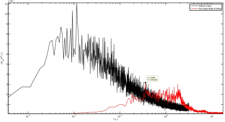
Back to the problem definition, figure 5.4 shows the non-dimensional one dimensional power spectra in longitudinal direction of the full scale Wall of Wind and the Silsoe Cube. The data which is used to create the power spectrum of the WoW is obtained during experiments with a 1:5 scale model of the Silsoe Cube. It is remarkable that the power spectrum of the WoW has no clear inertial subrange which is clearly visible in the Silsoe power spectrum. Although it should be investigated why there is no inertial subrange, this problem is not considered in this study. The WoW curve matches the Silsoe curve down to a reduced frequency of approximately 0.36. The measurements were conducted at a height of 1.2m, this results in a turbulence length scale of:

l= z

f =

1.2

0.36 = 3.33m (5.15)

The length scale of 3.33mis not even three times the size of their test building, the 1:5 scale model of the Silsoe Cube. This clearly shows the problem, as Richards [2013] suggested turbulence with a length scale up to ten times the building size should be modeled by the Wall of Wind.

10−3 ₁₀−2 ₁₀−1 ₁₀0 ₁₀1

1 2 3 4 5 6 7 8 9 10 11

x 10−3

X: 0.3598 Y: 0.003159

nS

uu

/U

2 (−)

f (−)

Silsoe Cube full scale Wall of Wind

6

Concept

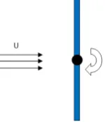
The proposed technique to generate turbulence is a passive rotating vane which can be seen as a flat plate on an axis, see figure 6.1. The vane is not controlled so the frequency at which the vane rotates depends on the dimensions of the vane and the mean flow velocity. The idea is to replace the static spires of the Wall of Wind by a number of vanes of different sizes in horizontal and vertical direction. The variety of vane size should encourage the generation of turbulence of different length scales. The principle behind the rotating vanes is the shedding of vortices. The flow approaching the vane will attach to the vane and as the vane rotates the flow will detach when the vane has rotated a certain angle.

Figure 6.1: Concept used to generate turbulence (viewed from top)

6.1

Literature

The literature study did not result in very much useful research papers. Most of the research done on turbulence generating techniques used active controlled vanes or used thin grids instead of rotating vanes. For example Nishi et al. [1999] used oscillating airfoils in the mid section of a wind tunnel to model the turbulence properties of the atmospheric boundary layer. Knebel et al. [2011] also used an active controlled method to model atmospheric wind field properties. The algorithm they used to control the rotation of the vanes is based on matching the probability density function (pdf) of the velocity increment of the generated flow with the pdf of the atmospheric wind field.

Previous done research showed promising results on using active controlled techniques to model the properties of the atmospheric wind field. Because the available time to do this project was limited it was not an option to design, build and test an active controlled setup, so the passive rotating vanes were used. Unfortunately there were no publications found of research on generating turbulence with multiple passive rotating vanes or anything strongly related.

6.2

First tests

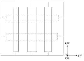
A simple test model was build to test the concept of passive rotating vanes. The test model is a 250mm square shaped wooden frame which holds three vertical vanes and two horizontal vanes, see figure 6.2. The vanes are created from corflute and their spans vary from approximately 20mmto 50mm. The vanes are basically flat plates which were attached on a steel rod which is able to rotate within the wooden frame.

The goal of the first tests was to get a first indication of the length scale and intensity of the turbulence which could be generated with passive rotating vanes. The tests were conducted in the Twisted Flow Wind Tunnel which is an open-jet wind tunnel, mainly used for yacht and bike testing. The wind tunnel is 7m wide, 3.5m high and 5.5m long with a maximum speed of 8.5m/s. The location of the test model was in the center of the tunnel and approximately 3mdownstream.

Figure 6.2: Test model

6.3

Concept test results

The Cobra Proce is placed 250mm downstream of the test model at a height of 125mm. The captured velocity data is used to calculate the power spectra. When the direction of the flow field is not within the range of ±45 deg the Cobra Probe is not able to capture the flow field. This could happen when a relatively large eddy passes the Cobra Probe. When the Cobra Probe fails in capturing the velocity components there will be zero values in the data set, these zero values are replaced by estimated velocities using interpolation. When more than 5% of the data are zero values the data is not used and the measurement is conducted again. Three configurations are tested: one vertical vane, three vertical vanes and three vertical vanes plus two horizontal vanes. Figure 6.3 shows the non-dimensional power spectra in all three orthogonal directions. The three tests are conducted at the same wind speed, the mean flow velocity downstream of the model is approximately 4m/s for the first configuration and 3m/s for the configurations which contain multiple vanes.

The first configuration does not generate very much turbulence, the area under the curves is quite small. There is a huge peak in the power spectra which corresponds to the frequency at which the vane rotates this peak means means there is a lot of turbulent kinetic energy at the corresponding frequency. There are no peaks in the power spectra of the configurations which use multiple vanes. Using more vanes increases the turbulence intensity as expected. It is remarkable that adding horizontal vanes to the setup increases the turbulent kinetic energy in the longitudinal and transverse direction, but does not increase the turbulent kinetic energy levels in vertical direction. The Suu and Svv curves shift upwards when the horizontal vanes are added to the test model but theSww curve does not shift significantly. This is probably due to the effect of the ground that limits turbulence in vertical direction. During the test period, also a few other configurations have been tested. It is observed that larger vanes cause higher turbulence intensities at a lower frequency. The power spectra corresponding to configurations which contain multiple vanes have their peak close to a reduced frequency of 0.2. Using the height at which the Cobra Probe is placed, the length scale of the turbulence is calculated: l=z/f = 0.125/0.2 = 0.63m. This length scale corresponds to four times the size of the test model that will be used in the final experiments, the 1:40 scale model of the Silsoe Cube.

10−2 ₁₀−1 ₁₀0 ₁₀1

0 0.005 0.01 0.015 0.02 0.025 0.03 0.035 0.04 0.045 0.05 f (−) nS/U

2 (−)

S

uu

S

vv

Sww

10−2 ₁₀−1 ₁₀0 ₁₀1

0 0.005 0.01 0.015 0.02 0.025 0.03 0.035 0.04 0.045 0.05 f (−) nS/U

2 (−)

S

uu

S

vv

Sww

10−2 ₁₀−1 ₁₀0 ₁₀1

0 0.005 0.01 0.015 0.02 0.025 0.03 0.035 0.04 0.045 0.05 f (−) nS/U

2 (−)

S

uu

S

vv

Sww

7

Wall of Wind scale model

This chapter introduces the built 1:8 scale model of the Wall of Wind. The chosen approach is explained and the results of the tests conducted in the Twisted Flow Wind Tunnel are discussed.

7.1

Scale model

The results of the test with the concept test model showed that high concentrations of turbulent kinetic energy at certain frequencies occur when a single vane is used. Therefore it is needed to use multiple vanes. The results also showed vanes rotating about a particular axis do not show higher turbulence intensities in a particular direction. It is also concluded that using vanes which rotate about different axes, to create equal like turbulence in multiple directions, is not needed.

The vanes which replace the spires in the 1:8 scale model of the WoW will be located further apart compared to the vanes in the concept test model. It is expected that the vortical structures created by the vanes will not interfere enough, so there will be energy peaks at certain frequencies. Hence the horizontal vanes will also be included in the scale model to break up the turbulent structures created by the vertical vanes. In the scale model, five vertical vanes and four horizontal vanes are used. The span of the vertical vanes varies from 75mm to 150mm and the span of the horizontal vanes varies from 70mm to 130mm. The maximum span is limited by the fact that it should be applicable at full scale. The spans are chosen to be as large as possible to generate as large turbulent structures as possible. The vanes are divided in multiple segments and the segments are deformed to encourage rotation in the flow. A vane with two segments is shown in figure 7.1.

Figure 7.1: A vane used in the WoW 1:8 scale model with two segments

(a) WoW 1:8 scale model with the spires configur-ation

(b) WoW 1:8 scale model with the vanes configur-ation

Figure 7.2: 1:8 scale model of the Wall of Wind

7.2

Approach

Because time was limited and the literature study did not provide much useful information it was decided use the trial-and-error approach. It would have been helpful if previous research provided fundamental laws or empirical relations related to the interaction of rotating flat plates in a uniform flow, but unfortunately this was not the case. During the first tests a lot of different configurations were tested and it was tried to find any relations between different vane configurations and the resulting power spectra. The tested configurations varied in number of vanes used, vanes at different locations and different number of segments. In the next section the most promising and remarkable configurations and their corresponding one dimensional power spectra will be discussed. The power spectra considered in this study are the power spectra in longitudinal direction, the only data available on the full scale WoW considered the longitudinal velocity component.

7.3

Turbulence measurements

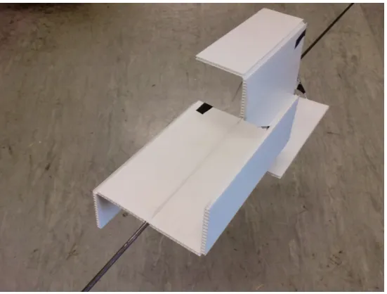
The first turbulence measurements were conducted in the Twisted Flow Wind Tunnel. Figure 7.3 shows the experimental setup. The WoW scale model which is basically a 1:8 scale model of the flow conditioning section is denoted by FCB (flow conditioning box). The FCB is located in the centre behind one of the fans (the wind tunnel has two fans). The Cobra Probe is placed at a certain distance behind the FCB. In horizontal direction the Cobra Probe is placed in the centre of the outlet of the FCB but at a height of 150mm. The height of 150mmcorresponds to the cube height of the 1:40 scale model of the Silsoe Cube that is used for the pressure measurements.

Figure 7.3: Test configuration in the Twisted Flow Wind Tunnel (Cobra Probe is marked by x)

the power spectrum down to a reduced frequency of 0.1. With the cube height known and the mean flow velocity known, which is equal to approximately 2m/s, the corresponding frequency can be calculated:

f =n·z

U ↔ n=

U·f

z =

2·0.1

0.15 = 1.33Hz (7.1)

For convenience, the frequency is set at 1Hz. It is needed to capture at least ten cycles of a certain frequency to get a reliable result corresponding to that frequency. At 1Hzthe required sampling time to capture ten cycles is ten seconds. For the averaging of the power spectra 25 blocks are used, so a sampling time of 250sis needed to get a power spectra which can be analysed down to a reduced frequency of 0.1. The used sampling frequency is 600Hz.

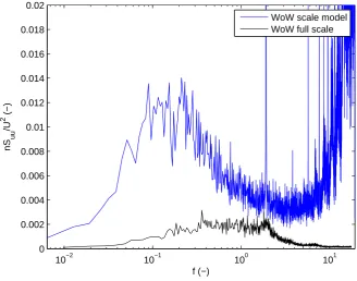
The first test is conducted with the spires configuration to compare the power spectra of the scale model with the full scale WoW. Figure 7.4 shows the longitudinal power spectra of the WoW scale model versus the full scale WoW. The spectra do not match at all which is probably due to the differences between the flows at the inlet of the FCB and the flow conditioning section. The major difference is the way the flow at the inlet is produced, the full scale WoW uses twelve huge fans and the flow is contracted directly. This creates a flow field which is different to the flow field created in the wind tunnel. A way to get better matching spectra, and thus a more realistic and better scale model, would be to match the Reynolds number and the Strouhal number. Unfortunately there was no data available about the Reynolds number or Strouhal number. associated with the full scale WoW. Also information about the turbulence spectra of the flow at the inlet of the flow conditioning section was not available. Even though the power spectrum of the WoW scale model does not match the full scale power spectrum, it matches the power spectrum of a scale model of the WoW which was tested in a wind tunnel by the researchers of the IHRC.

10−2 10−1 100 101

0 0.002 0.004 0.006 0.008 0.01 0.012 0.014 0.016 0.018 0.02

f (−)

nS

uu

/U

2 (−)

WoW scale model WoW full scale

Figure 7.4: Non-dimensional spectra of the WoW 1:8 scale model (Fs= 600Hz,Ts = 250s,B = 25) vs the full

scale WoW (Fs= 512Hz,Ts= 180s,B= 25)

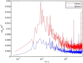
Figure 7.5 shows the one dimensional power spectra of the spires configuration and a vane configuration where all the vanes with all segments are used. The Cobra Probe is positioned 3500mm behind the outlet of the FCB. One eighth of the distance between the outlet of the flow conditioning section and the position where the turbulence measurements were conducted in the full scale case equals 700mm. In the first attempt, the measurement was conducted at 700mm, but the Cobra Probe was not able to capture the turbulent structures generate by the FCB with the full vanes configuration. Therefore the Cobra Probe had to be moved further away from the outlet of the FCB to be able to capture the turbulent structures of the generated flow field.

The turbulence intensity associated with the vanes configuration is higher compared to the spires configuration. It is remarkable that both power spectra have their peak around a reduced frequency of 0.1, but the the vane configuration shows a clear peak where the spires configuration shows a sort of flat top. The fact that the peaks of both spectra occur around the same reduced frequency indicates the generated turbulent structures are of the same order of size. The goal of this study is to test the rotating vanes technique and see whether it generates larger turbulent structures compared to the spires configuration. Hence, the spectrum of the vane configuration should shift to the left, to lower reduced frequencies. The turbulence intensities associated with the vane configuration are too high compared to the turbulence intensities which are measured at the Silsoe Cube experiments, therefore less vanes are used in the following tests.

10−2 10−1 100

0 0.002 0.004 0.006 0.008 0.01 0.012 0.014 0.016 0.018 0.02

f (−)

nS

uu

/U

2

Vanes Spires

Figure 7.5: Non-dimensional spectra of the full Vanes configuration vs the Spires configuration (both configura-tions: Fs= 600Hz,Ts= 250s, B= 25)

Figure 7.6 shows the difference between a configuration which has no horizontal vane positioned at the height of the Cobra Probe and a configuration which has. The red spectrum has a vane in front of the Cobra Probe and the black spectrum has not. It was expected that the eddies created by the vanes will interact with the flow which is not interfered by the vanes, which could end in the formation of a shear layer and higher turbulence intensities. This does not seem to be the case and the power spectra show that the test model, or in this case the Cobra Probe, should be in the wake of a vane to experience the generated turbulence.

10−2 10−1 100 0

0.002 0.004 0.006 0.008 0.01 0.012 0.014 0.016 0.018 0.02

f (−)

nS

uu

/U

2

Vanes center Vanes low

Figure 7.6: Non-dimensional spectra of two Vanes configurations considering vane position (both configurations: Fs= 600Hz,Ts= 250s, B= 25)

10−2 10−1 100

0 0.002 0.004 0.006 0.008 0.01 0.012 0.014 0.016 0.018 0.02

f (−)

nS

uu

/U

2

Vanes (2100mm) Spires (700mm)

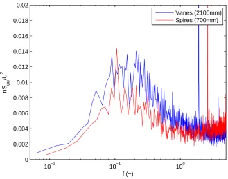
Figure 7.7: Non-dimensional spectra the Vanes configuration at 2100mm vs the Spires configuration at 700mm (both configurations: Fs= 600Hz,Ts= 250s, B= 25)

8

Open-jet facility

To create an open-jet facility a contraction has been built which can be used in the closed-loop wind tunnel of the University of Auckland, the De Bray wind tunnel. This chapter discusses the turbulence and pressure measurements which were conducted in the De Bray wind tunnel.

8.1

Turbulence measurements

The De Bray wind tunnel is a closed-loop wind tunnel which is 1.8m wide and 1.1m high. The built contraction can be placed in the wind tunnel and contracts the flow to the cross sectional area of the FCB which is 762mmwide and 533mmhigh. The turbulence measurements which were conducted in the Twisted Flow Wind Tunnel were also carried out in the De Bray wind tunnel to study differences in the power spectra corresponding to both test configurations.

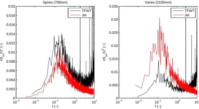
Figure 8.1 shows the power spectra of the spires configuration at 700mmand the best vane configuration at 2100mm, discussed in the previous chapter. The red curves represent the power spectra of the same configurations, measured at the same distance behind the outlet of the FCB. It is remarkable that the power spectrum corresponding to the spires configuration is shifted downwards and the power spectrum corresponding to the vane configuration is shifted upwards. Considering the spires configuration, the flow generated with the open jet facility contains less turbulent kinetic energy compared to the flow generated with the vanes, but for the vane configuration the opposite is true. Using the Cobra Probe, a few turbulence measurements were conducted at different positions and the results indicate the formation of a shear layer between the flow which leaves the FCB and the stagnant air around the outlet of the FCB. This shear layer contains high turbulence intensities and develops downstream. When the Cobra Probe is positioned 2100mmbehind the outlet of the FCB at a height of 150mm, it seems that the Cobra Probe is positioned in the shear layer and therefore the resulting power spectrum shows high turbulence intensities. This explains the difference in the shift of the power spectrum. It also imposes a restriction on the area behind the FCB which can be used to conduct measurements, because results which are influenced by the shear layer are not usable.

10−3 10−2 10−1 100 101 0

0.002 0.004 0.006 0.008 0.01 0.012 0.014 0.016 0.018 0.02

f (−)

nS

uu

/U

2 (−)

Spires (700mm)

10−3 10−2 10−1 100 101 0

0.005 0.01 0.015 0.02 0.025 0.03 0.035

f (−)

nS

uu

/U

2 (−)

Vanes (2100mm)

TFWT Jet

TFWT Jet

Figure 8.1: Non-dimensional spectra Spires and Vane configuration: Jet facility (Fs = 625Hz, Ts = 250s,

Using the best vane configuration of the series of tests which were conducted at the Twisted Flow Wind Tunnel, a new series of tests has been carried out to find a vane configuration which results in a power spectrum at significant lower frequencies. The same approach is used and the different tested vane setups varied in number of vanes used, different number of segments used and vanes at different locations. It was observed that it is essential to use two layers of vanes, the second layer of vanes is needed to break up the vortical structures created by the first layer of vanes. It is also important to position the vanes uniformly throughout the cross sectional area of the FCB to create a flow with uniform turbulence characteristics. This is due to the interaction between the flow around the vanes and the flow which does not pass a vane, this interaction is weak. This was also discussed in the previous chapter.

The best vane configuration is shown in figure 8.2 and the corresponding power spectra is shown in figure 8.3. It was not possible to find a vane configuration which resulted in a power spectrum at significant lower frequencies compared to the power spectrum of the spires configuration. This is mainly due to the fact that the rotational frequency of the vanes is too high and can not be controlled. This same problem was discussed in the previous chapter. It was tried to slow the vanes down by using segments which encourage the vane to rotate in counter direction, but this did not made a significant difference.

Figure 8.2: Vane configuration 2

10−2 10−1 100 101

2 4 6 8 10 12 14 16 18

x 10−3

f (−)

nS

uu

/U

2 (−)

Spires Vanes

The vane configuration shown in figure 8.2 is not uniform at all. Although it results in a relatively good power spectrum in the centre at a height of 150mm, the power spectra at other positions will be worse. Figure 8.4 shows the power spectra which were created using Cobra Probe measurements at different positions. The power spectra at a height of 400mmboth show a high peak in the turbulent kinetic energy at a certain frequency. The 1:40 scale model of the Silsoe Cube has a length of 150mm and therefor in this case the power spectrum at 400mm does not matter, but there will also be structures with other dimensions which will be tested in the full scale Wall of Wind. In that case a flow with more uniform turbulence characteristics is required.

10−2 100

0 0.005 0.01 0.015 0.02 f (−) nS uu /U 2

400mm height, center

10−2 100

0 0.005 0.01 0.015 0.02 f (−) nS uu /U 2

400mm height, 250mm right

10−2 100

0 0.005 0.01 0.015 0.02 f (−) nS uu /U 2

150mm height, center

10−2 100

0 0.005 0.01 0.015 0.02 f (−) nS uu /U 2

150mm height, 250mm right

Figure 8.4: Non-dimensional spectra of Vane configuration (Fs = 625Hz, Ts = 250s, B = 25) considering

uniformity

A few more turbulence measurements were conducted with different vane configurations to find a con-figuration which resulted in a flow with more uniform turbulence characteristics. Figure 8.5 shows this vane configuration and figure 8.6 shows the corresponding power spectra at a few positions around the scale model of the Silsoe Cube, 1H represents one time cube height. The power spectra show that the turbulence characteristics of the flow are quite uniform. It was observed that the direction of rotation of the vanes influences the blockage effect created by the vanes. The vanes are shaped in a curved way to encourage rotation, the flow which passes along the side of the vane which rotates downstream experiences more blockage than the flow which passes along the other side of the vane.

Figure 8.5: Vane configuration 1

10−2 100

0 0.01 0.02 0.03 f (−) nS uu /U

2 (−)

1.5H height, 1H left

10−2 100

0 0.01 0.02 0.03 f (−) nS uu /U

2 (−)

1.5H height, center

10−2 100

0 0.01 0.02 0.03 f (−) nS uu /U

2 (−)

1.5H height, 1H right

10−2 100

0 0.01 0.02 0.03 f (−) nS uu /U

2 (−)

1H height, 1H left

10−2 100

0 0.01 0.02 0.03 f (−) nS uu /U

2 (−)

1H height, center

10−2 100

0 0.01 0.02 0.03 f (−) nS uu /U

2 (−)

1H height, 1H right

10−2 100

0 0.01 0.02 0.03 f (−) nS uu /U

2 (−)

0.5H height, 1H left

10−2 100

0 0.01 0.02 0.03 f (−) nS uu /U

2 (−)

0.5H height, 1H center

10−2 100

0 0.01 0.02 0.03 f (−) nS uu /U

2 (−)

0.5H height, 1H right

Figure 8.6: Non-dimensional spectra of the more uniform Vanes setup (Fs = 625Hz, Ts = 250s, B = 25)

100 0 0.005 0.01 0.015 0.02 f (−) nS uu /U

2 (−)

1.5H height, 1H left

Silsoe FS Spires 100 0 0.005 0.01 0.015 0.02 f (−) nS uu /U

2 (−)

1.5H height, center

100 0 0.005 0.01 0.015 0.02 f (−) nS uu /U

2 (−)

1.5H height, 1H right

100 0 0.005 0.01 0.015 0.02 f (−) nS uu /U

2 (−)

1H height, 1H left

100 0 0.005 0.01 0.015 0.02 f (−) nS uu /U

2 (−)

1H height, center

100 0 0.005 0.01 0.015 0.02 f (−) nS uu /U

2 (−)

1H height, 1H right

100 0 0.005 0.01 0.015 0.02 f (−) nS uu /U

2 (−)

0.5H height, 1H left

100 0 0.005 0.01 0.015 0.02 f (−) nS uu /U

2 (−)

0.5H height, 1H center

100 0 0.005 0.01 0.015 0.02 f (−) nS uu /U

2 (−)

0.5H height, 1H right

Figure 8.7: Non-dimensional spectra of Silsoe Cube full scale vs Spires configuration (Fs = 625Hz, Ts = 250s,

B= 25) considering uniformity

8.2

Pressure measurements

Pressure measurements were conducted using the 1:40 scale model of the Silsoe Cube. The first goal of the pressure measurements was to get insight in the relation between the power spectra of the corresponding flow field and the pressures produced by the flow on the Silsoe Cube model. Although the configura-tions with the vanes do not create the low-frequent turbulence which was hoped for, the insight in the relationship between the turbulence characteristics and the pressures could be useful for further research. The second goal was to see whether the pressures which result from the spires configuration match the pressures of the full scale Silsoe case. The tested vane configurations will be denoted by vane configuration 1, 8.5, and vane configuration 2, 8.2.

The pressure measurements were conducted over a range of 180◦at intervals of 5◦ for all three configura-tions. Using symmetry the cases for all angles from 0◦ to 360◦ can be constructed. The data is sampled at a frequency of 600Hzand a sampling time of 120s. The raw pressure data is corrected for the length of the tubes using a recursive filter. With the resulting pressures the mean, maximum and minimum pressure coefficients are calculated:

Cp= p q

ˆ Cp=

ˆ p ˆ q

ˇ Cp=

ˇ p ˆ

q (8.1)

The maximum and minimum pressure are calculated using the maximum dynamic pressure ˆqbecause this is also done by Richards and Hoxey [2012a] with the full scale Silsoe data.

(a) Complete setup (b) 1:40 scale model of the Silsoe Cube

Figure 8.8: Experimental setup for pressure measurements

Measuring the pressures at 90 taps and at 36 different angles results in a lot of data. As it does not make sense to analyse all the different cases it is chosen to analyse a few cases which have been considered in previous research on the full scale Silsoe Cube. Figure 8.9 shows the pressure tap configurations which are considered. The mean, maximum and minimum pressures on the horizontal and vertical ring are considered for the case where the flow angleθis equal to 0◦and 45◦. For the roof configuration, the mean pressure coefficients are considered for flow angles of 0◦ and 45◦.

(a) Horizontal ring (b) Vertical ring (c) Roof

10−3 10−2 10−1 100 101 2

4 6 8 10 12 14 16 18

x 10−3

f (−)

nS

uu

/U

2

Spires

Vanes Config. 2 Vanes Config. 1 Silsoe FS

Figure 8.10: Non-dimensional spectra of the Silsoe Cube full scale, the Spires setup and the two Vanes setups (Fs= 625Hz,Ts= 250s,B= 25)

Figure 8.10 shows the non-dimensional longitudinal power spectra of the two vane configurations and the spires configuration in comparison with the power spectrum of the full scale Silsoe Cube experiment. The configuration with the spires creates the lowest turbulence intensities. The power spectra of the two vane configurations are quite similar except for the fact that the power spectrum of vane configuration 2 shows more low frequent turbulence. Therefore it is interesting to study the resulting pressures on the test model using these two vane configurations. For the one dimensional power spectra in all three directions for all three configurations see appendix B.

Like the power spectra also the differences in velocity profiles and turbulence intensity profiles can explain differences in the resulting pressure distributions on the test model. The velocity profiles and the turbu-lence intensity profiles for the three test configurations in comparison with the Silsoe data are shown in figure 8.11.

ˆ The velocity profiles show fairly good agreement up to 1H, the roughness elements, which are used in all three configurations, probably play a major role in creating the velocity boundary layer.

ˆ Vane configuration 1 shows a very linear velocity profile and not an expected power law.

ˆ Above 1H, vane configuration 1 shows good agreement with the full scale Silsoe data, whereas the velocities for other two configurations show higher velocities compared to the Silsoe data.

ˆ Considering the longitudinal turbulence intensity, there is good agreement between vane configura-tion 1 and the Silsoe data. The spires configuraconfigura-tion differs the most from the Silsoe data and vane configuration 2 shows good agreement up to 1H.

ˆ Considering the transverse turbulence intensity not one of the three configurations shows really agreement with the Silsoe data. The spires configuration only matches from the ground up to 0.5H. Vane configuration 2 has intensities which are closest to the Silsoe data but the vane configuration 1 obeys a power law similar to the Silsoe data.

Summarizing: the velocity profiles show fairly good agreement up to 1H, although vane configuration 1 shows a linear profile instead of an expected power law. Considering the three turbulence intensity profiles, the turbulence intensity profiles of the Silsoe experiment are not matched, but vane configuration 1 shows the best agreement considering the profile.

0.8 1 1.2 1.4

0 0.5 1 1.5 2 2.5 3 Velocity profiles u/U (−) z/H (−)

0 5 10 15 20 25

0 0.5 1 1.5 2 2.5 3

Longitudinal turbulence intensity profiles

I_uu (%)

z/H (−)

0 5 10 15 20 25

0 0.5 1 1.5 2 2.5 3

Transverse turbulence intensity profiles

I

vv (%)

z/H (−)

0 5 10 15 20 25

0 0.5 1 1.5 2 2.5 3

Vertical turbulence intensity profiles

I

ww (%)

z/H (−)

Silsoe WOW VC1 VC2

Figure 8.11: Velocity and turbulence intensity profiles

8.2.1

Mean

C

horizontal ring

Figure 8.12 shows the mean pressure coefficients on the horizontal ring for both cases. Considering the case where the flow angle equals 0◦:

ˆ The third pressure tap on the horizontal ring did not work properly so this one is left out in the graph.

ˆ The spires configuration and vane configuration 2 show quite good agreement on the windward surface of the test model. Using vane configuration 1 results in higher mean pressure coefficients. The two vane configurations clearly create a flow which has not a mean flow angle of 0◦ _{deg. This}

is shown by the asymmetry in the pressure coefficients on the windward surface.

ˆ Considering the side surfaces and leeward surface of the model we see that the flow for the two vane configurations is skewed, the pressure coefficients on the two side surface do not show symmetry as we see with the Silsoe data and the spires configuration.

ˆ The suctions on the leeward surface generated by the three configurations show fairly good agreement with the Silsoe data, but the higher suctions on the side surfaces are not matched.

And considering the case where the flow angle equals 45◦:

ˆ Vane configuration 1 and vane configuration 2 clearly show skewness in the flow considering the two windward surfaces.

ˆ The peak suctions which occur in the middle of the leeward surfaces in the Silsoe are not modeled by one of the three configurations.

0 0.5 1 1.5 2 2.5 3 3.5 4

−1 −0.5 0 0.5 1 1.5

s/H (−)

C p

(−)

Mean C

p horizontal ring 0 o

Silsoe WOW VC1 VC2

(a) Mean pressure coefficients on the horizontal ring forθ= 0◦

0 0.5 1 1.5 2 2.5 3 3.5 4

−0.8 −0.6 −0.4 −0.2 0 0.2 0.4 0.6 0.8

s/H (−)

C p

(−)

Mean C

p horizontal ring 45 o

Silsoe WOW VC1 VC2

(b) Mean pressure coefficients on the horizontal ring forθ= 45◦

8.2.2

Maximum and minimum

C

horizontal ring

Figure 8.13 shows the maximum and minimum pressure coefficients on the horizontal ring for both cases. Considering the case where the flow angle equals 0◦:

ˆ The graphs show two series for every case, the series with the higher values are the maximum pressure coefficients and the series with the lower values are the minimum pressure coefficients.

ˆ The maximum pressure coefficients show fairly good agreement on the side surfaces and the leeward surface. The minimum pressure coefficients show fairly good agreement on the windward surface and the leeward surface.

ˆ On the side surfaces, the minimum pressure coefficients shows the same behaviour as the mean pressure coefficients. The Silsoe data shows clearly flow reattachment behavior and so does the spires configuration. The two vane configurations show more constant minimum pressure coefficients. The high suctions which were not matched considering the mean pressure coefficients are better matched considering these values for the minimum pressure coefficients. The pressure coefficients of the Silsoe data are not completely matched by the spires configuration, but at least they are greater in magnitude.

ˆ The second-last pressure tap of the spires configuration gives a value for the minimum pressure coefficient which does not seem realistic. There was probably something wrong with the pressure tap on the pressure model during the run.

And considering the case where the flow angle equals 45◦:

ˆ The spires configuration, which showed a bit of flow separation and reattachment behaviour for the 0◦ flow angle case, does not show this behaviour for the 45◦ flow angle case. The flow separation and reattachment behaviour is clearly present in the Silsoe data, this can be seen by looking at the gradient in the pressure coefficient along the windward surfaces. The spires configuration now shows more constant maximum and minimum pressure coefficients as was seen earlier in with the two vane configurations. This is probably due to the fact that the acceleration of the flow is lower in the 45◦

flow angle case.

ˆ The peak suctions, which occur on the leeward surfaces, are not matched but they are higher which is better than the case in which they are lower.

8.2.3

Mean

C

vertical ring

Figure 8.14 shows the mean pressure coefficients on the vertical ring for both cases. Considering the case where the flow angle equals 0◦:

ˆ The data for the first and last tap for the Silsoe case is not shown as this data is not available.

ˆ The pressure coefficients on the windward surface of the full scale Silsoe case are best matched by the spires configuration and vane configuration 1 shows the worst match. Considering the turbulence intensity profiles from the ground up to 1H, it is clear that the turbulence intensities corresponding to the spires configuration are the closest to the full scale Silsoe case and the turbulence intensity profiles corresponding to vane configuration show the worst match.

ˆ The high suction on the beginning of the roof is matched by all three configurations. The three configurations show earlier reattachment of the flow by quick rising mean pressure coefficients com-pared to the Silsoe case. This is due to the higher vertical turbulence intensities at 1H as turbulence encourages flow reattachment.

ˆ The mean pressure coefficients on the leeward surface show quite good agreement.

And considering the case where the flow angle equals 45◦:

0 0.5 1 1.5 2 2.5 3 3.5 4 −2

−1.5 −1 −0.5 0 0.5 1 1.5 2

s/H (−)

C p

(−)

Max/Min C

p horizontal ring 0 o

Silsoe WOW VC1 VC2

(a) Maximum and minimum pressure coefficients on the horizontal ring forθ= 0◦

0 0.5 1 1.5 2 2.5 3 3.5 4

−1.5 −1 −0.5 0 0.5 1 1.5 2

s/H (−)

C p

(−)

Max/Min C

p horizontal ring 45 o

Silsoe WOW VC1 VC2

(b) Maximum and minimum pressure coefficients on the horizontal ring forθ= 45◦

0 0.5 1 1.5 2 2.5 3 −1.5

−1 −0.5 0 0.5 1 1.5

s/H (−)

C p

(−)

Mean C

p vertical ring 0 o

Silsoe WOW VC1 VC2

(a) Mean pressure coefficients on the vertical ring forθ= 0◦

0 0.5 1 1.5 2 2.5 3

−2 −1.5 −1 −0.5 0 0.5 1

s/H (−)

C p

(−)

Mean C

p vertical ring 45 o

Silsoe WOW VC1 VC2

(b) Mean pressure coefficients on the vertical ring forθ= 45◦

8.2.4

Maximum and minimum

C

vertical ring

0 0.5 1 1.5 2 2.5 3

−3 −2.5 −2 −1.5 −1 −0.5 0 0.5 1 1.5 2

s/H (−)

C p

(−)

Max/Min C

p vertical ring 0 o

Silsoe WOW VC1 VC2

(a) Maximum and minimum pressure coefficients on the vertical ring forθ= 0◦

0 0.5 1 1.5 2 2.5 3

−2 −1.5 −1 −0.5 0 0.5 1 1.5

s/H (−)

C p

(−)

Max/Min C

p vertical ring 45 o

Silsoe WOW VC1 VC2

(b) Maximum and minimum pressure coefficients on the vertical ring forθ= 45◦

Figure 8.15: Maximum and minimum pressure coefficients on the vertical ring

Figure 8.15 shows the maximum and minimum pressure coefficients on the vertical ring for both cases. Considering the case where the flow angle equals 0◦_:

ˆ The maximum and minimum pressure coefficients show overall better agreement on the vertical ring than the maximum and minimum pressure coefficients on the horizontal ring.

ˆ The minimum pressure coefficients corresponding to the spires configuration and vane configuration 1 show fairly good agreement with the full scale Silsoe data. Vane configuration 2 produces a very high peak suction at the beginning of the roof.

ˆ The last pressure tap in case of the spires configuration and vane configuration 2 show a very high suction, this is probably due to a flaw in the pressure tap or pressure module during that run.

And considering the case where the flow angle equals 45◦:

ˆ The maximum and minimum pressure coefficients on the vertical ring for the 45◦ flow angle case show less overall agreement than the pressure coefficients in the 0◦ flow angle case.

ˆ Vane configuration 2 shows very high peak suctions on the windward surface compared to the other configurations and the full scale Silsoe case.

ˆ Vane configuration 2 and the spires configuration are capable of producing the high suction on the beginning of the roof, but the minimum pressure coefficients from the beginning of the roof on do not match. Vane configuration 1 is not able to produce a high enough suction, but the minimum pressures show better agreement compared to the Silsoe case.

ˆ The peak pressures show overall fairly good agreement.

8.2.5

Mean

C

roof

y/H (−)

x/H (−) Silsoe FS

0.2 0.4 0.6 0.8

0.2 0.4 0.6 0.8

y/H (−)

x/H (−) WOW

0.2 0.4 0.6 0.8

0.2 0.4 0.6 0.8

y/H (−)

x/H (−) VC1

0.2 0.4 0.6 0.8

0.2 0.4 0.6 0.8

−1.4 −1.2 −1 −0.8 −0.6 −0.4 −0.2 0 0.2

Mean C

p

roof 0

o

y/H (−)

x/H (−) VC2

0.2 0.4 0.6 0.8

0.2 0.4 0.6 0.8

Figure 8.16: Mean pressure coefficients on the roof forθ= 0◦

other configurations. The contour shapes close to the windward sides of the roof indicate the formation of conical vortices at the beginning of the roof. The suctions associated with vane configuration 1 seem to be higher than the suctions which are shown in figure 8.14, this may not be the case as both graphs are based on the same pressure taps. This small deviation can be explained by the fact that the contour plots of the roof are based on data from different test runs and symmetry is used whereas figure 8.14 is based on just one data set. There was no time left to correct for this deviation.

y/H (−)

x/H (−) Silsoe FS

0.2 0.4 0.6 0.8

0.2 0.4 0.6 0.8

y/H (−)

x/H (−) WOW

0.2 0.4 0.6 0.8

0.2 0.4 0.6 0.8

y/H (−)

x/H (−) VC1

0.2 0.4 0.6 0.8

0.2 0.4 0.6 0.8

−2 −1.5 −1 −0.5 0

Mean C

p

roof 45

o

y/H (−)

x/H (−) VC2

0.2 0.4 0.6 0.8

0.2 0.4 0.6 0.8

Figure 8.17: Mean pressure coefficients on the roof forθ= 45◦

8.2.6

Summary

Conclusion

The goal of this study was:

Find and test a technique which can be used to model low-frequency large-scale turbu-lence with the Wall of Wind.

Unfortunately, it is concluded that the proposed technique, passive rotating vanes, does not create low-frequency turbulence with a length scale up to ten times the building size. The main problem seems to be the dependence of the rotational frequency of the vanes on the mean flow velocity. It was observed that vanes which rotate at a lower angular frequency generate velocity fluctuations at lower frequencies. Hence, if the angular frequency of the vanes could be controlled, thus it does not depend on the flow velocity, it might be possible to generate larger turbulent structures at relatively high flow velocities. Previous done research on turbulence generation using controlled mechanisms showed promising results, see chapter 6. It is recommended to test the possibilities of controlled vanes with a basic experiment because it is not very time-consuming and the results could be very useful.

If one decides to use (passive) rotating vanes to generate turbulence, ons must know:

ˆ The rotation of the vanes causes skewness in the flow as was shown in the results of the pressure measurements. It is expected that skewness could be limited by using smaller vanes.

ˆ To avoid high levels of turbulent kinetic energy at certain frequencies (peaks in the power spectra), one should use multiple layers of vanes to break up the created turbulent structures. It is expected that peaks can also be avoided by using smaller vanes as smaller vanes will generate lower turbulence intensities.

ˆ The results of the turbulence measurements conducted at the Twisted Flow Wind Tunnel showed that there is only a weak interaction between the flow which is disturbed by a vane and the flow which passes through a ’gap’ in the layer of vanes. Hence, one should use enough vanes to disturb all the incoming flow or use multiple layers, otherwise the turbulence characteristics of the flow will not be uniform throughout the cross-sectional area.

Besides the study on the vanes, the spires configuration which is currently used in the Wall of Wind was also studied. The comparison of the longitudinal one dimensional power spectrum of the WoW with the Silsoe data showed there is indeed a lack of generated low-frequency turbulence. The power spectrum of the WoW did not show a typical sub inertial range, which could be due to the turbulent flow not being in equilibrium, this should be investigated.

Bibliography

A.M. Aly, A. Gan Chowdhury, and G. Bitsuamlak. Wind profile management and blockage assessment for a new 12-fan wall of wind facility at fiu. Wind and Structures, 14(4):285–300, 2011.

S Fong. The strcuture of equilibrium turbulent boundary layers, 1995.

P Knebel, A Kittel, and J. Peinke. Atmospheric wind field conditions generated by active grids. Exp. Fluids, 51:471–481, 2011.

A.N. Kolmogorov. The local structure of turbulence in incompressible viscous fluid for very large reynolds numbers. Comptes rendus (Doklady) de l’Academie des sciences de l’U.R.S.S., (30):301–305, 1941. from editors ’Turbulence, classical papers on statistical theory’,edited by Friedlander, S.K. and Topper, L., Interscience Pub., 1961, pp. 151-155.

A. Nishi, H. Kikugawa, Y. Matsuda, and D. Tashiro. Active control of turbulence for an atmospheric boundary layer model in a wind tunnel. Journal of Wind Engineering and Industrial Aerodynamics, 83: 409–419, 1999.

P.J. Richards. Requirements for modelling low-rise buildings at large-scales in the wall of wind, 2013.

P.J. Richards and R.P. Hoxey. Pressures on a cubic building - part 1: Full-scale results. Journal of Wind Engineering and Industrial Aerodynamics, 102:72–86, 2012a.

P.J. Richards and R.P. Hoxey. Pressures on a cubic building - part 2: Quasi-steady and other processes.

Journal of Wind Engineering and Industrial Aerodynamics, 102:87–96, 2012b.

P.J. Richards, R.P. Hoxey, and L.J. Short. Wind pressures on a 6 m cube. Journal of Wind Engineering and Industrial Aerodynamics, 89(14-15):1553–1564, 2001.

P.J. Richards, R.P. Hoxey, B.D. Connell, and D.P. Lander. Wind tunnell modelling of the silsoe cube.

Journal of Wind Engineering and Industrial Aerodynamics, 95:1384–1399, 2007.

G.I. Taylor. The spectrum of turbulence. Proceeding of the Royal Society, (A164):476–490, 1938. from ’Turbulence, classical papers on statistical theory’, edited by Friedlander, S.K. and Topper, L., Inter-science Pub., 1961, pp. 100-114.

A

Spectral analysis Matlab script

1 function [ u f psdu ] = S p e c t r a l A n a l y s i s ( u , SampleFrequency , B l o c k S i z e ) 2

3 %Determine t h e number o f d a t a p o i n t s i n u

4 N = length( u ) ;

5

6 %+++++IF THERE ARE ZERO VALUES IN THE DATA, USE INTERPOLATION TO SET A REAL VALUE+++++

7 %C r e a t e a v e c t o r w i t h t h e i n d i c e s o f a l l t h e non z e r o e l e m e n t s i n u 8 NonZeroElements = f i n d( u ) ;

9 %I g n o r e d a t a a t t h e b e g i n n i n g and t h e end w h i c h h a v e z e r o v a l u e 10 u = u ( NonZeroElements ( 1 ) : NonZeroElements (end) ) ;

11 %R e c r e a t e a v e c t o r w i t h t h e i n d i c e s o f a l l t h e non z e r o e l e m e n t s i n u 12 NonZeroElements = f i n d( u ) ;

13 %Loop t h r o u g h t h e e l e m e n t s o f u t o f i n d t h e z e r o v a l u e s 14 f o r i = 1 :length( NonZeroElements )−1

15 i f( NonZeroElements ( i +1)−NonZeroElements ( i )>1) %I f t h e d i f f e r e n c e b e t w e e n two c o n s e c u t i v e e l e m e n t s i s g r e a t e r t h a n 1 , t h e r e must b e

a z e r o v a l u e b e t w e e n them

16 NumberOfZeroValues = NonZeroElements ( i +1)−NonZeroElements ( i )−1;

%C a l c u l a t e t h e number o f z e r o v a l u e s b e t w e e n them 17 u ( NonZeroElements ( i ) : NonZeroElements ( i +1) ) = l i n s p a c e( u (

NonZeroElements ( i ) ) , u ( NonZeroElements ( i +1) ) ,

NumberOfZeroValues +2) ; %R e p l a c e t h e z e r o v a l u e w i t h a l i n e a r i n t e r p o l a t e d v a l u e

18 end

19 end

20

21 %+++++SPLIT THE DATA IN BLOCKS OF SIZE EQUAL TO THE SET BLOCKSIZE+++++ 22 %C a l c u l a t e t h e number o f b l o c k s

23 NumberOfBlocks = f l o o r(N/ B l o c k S i z e )

24 %D e c l a r e a m a t r i x t o s t o r e t h e b l o c k s i n t h e columns 25 uu = zeros( B l o c k S i z e , NumberOfBlocks ) ;

26 f o r i = 1 : NumberOfBlocks

27 uu ( : , i ) = u ( ( 1 + ( i−1)*B l o c k S i z e ) : i*B l o c k S i z e ) ; %Each column o f t h e m a t r i x u c o n t a i n s a b l o c k o f d a t a w i t h s i z e B l o c k S i z e

28 end

29 u = u ( 1 : NumberOfBlocks*B l o c k S i z e ) ; 30

31 %+++++FOURIER TRANSFORM THE BLOCKS, CALCULATE PSD, CHECK IF THE VARIANCE OF THE TIME HIST . MATCHES THE AREA UNDER PSD CURVE AND THEN AVERAGE +++++

32 %S e t N e q u a l t o t h e B l o c k S i z e f o r t h e F o u r i e r t r a n s f o r m a t i o n and p r o c e s s i n g o f t h e t r a n s f o r m e d d a t a

33 N = B l o c k S i z e ;

34 %D e c l a r e a m a t r i x t o s t o r e t h e F o u r i e r t r a n s f o r m e d d a t a 35 psduu = zeros(N/2+1 , NumberOfBlocks ) ;

36 %Loop t h r o u g h a l l t h e columns o f uu and d e t e r m i n e t h e F o u r i e r t r a n s f o r m f o r e a c h b l o c k

37 f o r i = 1 : NumberOfBlocks

40 f f t u = f f t(U) ; %F o u r i e r t r a n s f o r m t h e d a t a o f u

41 f f t u = f f t u ( 1 :N/2+1) ; %Throw away s e c o n d h a l f o f t h e d a t a b e c a u s e o f symmetry

42 psdu = 1 / ( SampleFrequency*N)*abs( f f t u ) . ˆ 2 ; %C a l c u l a t e t h e power s p e c t r a l d e n s i t y

43 psdu ( 2 :end−1) = 2*psdu ( 2 :end−1) ; %M u l t i p l y t h e d a t a w i t h a f a c t o r 2 e x c e p t f o r t h e z e r o f r e q u e n c y and t h e N y q u i s t f r e q u e n c y

44 psduu ( : , i ) = psdu ; %S e t t h e i t h column o f psduu e q u a l t o t h e PSD d a t a o f t h e i t h column o f uu

45

46 %Determine t h e a r e a under t h e p s d c u r v e

47 psduArea = 0 ;

48 f o r j = 2 :length( psdu )−1

49 psduArea = psduArea+psdu ( j )*( SampleFrequency /N) ;

50 end

51 %I f t h e a r e a under t h e p s d c u r v e i s n o t w i t h i n 1% e q u a l t o t h e v a r i a n c e o f t h e t i m e h i s t o r y r e c o r d d i s p l a y e r r o r

52 i f( psduArea / u V a r i a n c e>1.001 | | psduArea / u V a r i a n c e<0 . 9 9 9 )

53 d i s p l a y ( ’ERROR IN SPECTRAL ANALYSIS , AREA UNDER PSD CURVE DOES

NOT MATCH VARIANCE OF TIME HISTORY DATA ’ )

54 end

55

56 end

57 %Average t h e F o u r i e r t r a n s f o r m e d d a t a 58 psdu = mean( psduu , 2 ) ;

59

60 %+++++CREATE A FREQUENCY VECTOR AND IGNORE THE ZERO FREQUENCY+++++ 61 %Due t o a l i a s i n g we can o n l y u s e t h e d a t a up t o t h e N y q u i s t f r e q u e n c y 62 f = ( 0 : SampleFrequency /N: SampleFrequency / 2 ) ’ ;

63 %D e l e t e t h e z e r o f r e q u e n c y o u t o f t h e p s d and f r e q u e n c y v e c t o r 64 f = f ( 2 :end) ; psdu = psdu ( 2 :end) ;

B

Power spectra of the Spires configuration

and the Vane configurations

10−2 10−1 100 101

1 2 3 4 5 6 7 8 9x 10

−3

f (−)

nS/U

2

S_uu

S

vv

S_ww

Figure B.1: Non-dimensional spectra of the Spires configuration, all three components (Fs= 625Hz,Ts= 250s,

10−2 10−1 100 101 2

4 6 8 10 12

x 10−3

f (−)

nS/U

2

S

uu

S_vv

S

ww

Figure B.2: Non-dimensional spectra of Vane Configuration 1, all three components (Fs = 625Hz, Ts = 250s,

B= 30)

10−2 10−1 100 101

2 4 6 8 10 12 14 16 18

x 10−3

f (−)

nS/U

2

S

uu

S_vv

S_ww

Figure B.3: Non-dimensional spectra of Vane Configuration 2, all three components (Fs = 625Hz, Ts = 250s,

C

Standard deviations of pressure coefficients

0 0.5 1 1.5 2 2.5 3 3.5 4

0 0.2 0.4 0.6 0.8 1 1.2 1.4

s/H (−)

C p

(−)

Standard deviation C_p horizontal ring 0o

Silsoe WOW VC1 VC2

(a) Standard deviations of pressure coefficients on the horizontal ring forθ= 0◦

0 0.5 1 1.5 2 2.5 3 3.5 4

0 0.2 0.4 0.6 0.8 1 1.2 1.4

s/H (−)

C p

(−)

Standard deviation C_p horizontal ring 45o

Silsoe WOW VC1 VC2

(b) Standard deviations of pressure coefficients on the horizontal ring forθ= 45◦

0 0.5 1 1.5 2 2.5 3 0

0.1 0.2 0.3 0.4 0.5 0.6 0.7 0.8 0.9 1

s/H (−)

C p

(−)

Standard deviation C_p vertical ring 0o

Silsoe WOW VC1 VC2

(a) Standard deviations of pressure coefficients on the vertical ring forθ= 0◦

0 0.5 1 1.5 2 2.5 3

0 0.2 0.4 0.6 0.8 1 1.2 1.4 1.6 1.8

s/H (−)

C p

(−)

Standard deviation C

p vertical ring 45 o

Silsoe WOW VC1 VC2

(b) Standard deviations of pressure coefficients on the vertical ring forθ= 45◦