Calculating Scattering Matrices by Wave
Function Matching on Cu-Co interfaces
Vincent Bosboom
University of Twente
July 4, 2018
Abstract
In this paper the spin-dependent transmission through an ideal copper-cobalt interface is calculated using the method of wavefunc-tion matching (WFM) implemented with a basis of muffin-tin or-bitals (MTO) within the framework of density functional theory (DFT). A sketch of DFT is given and the theory of muffin-tin or-bitals is explained, illustrated with examples of vanadium, copper and cobalt bands structures.
Keywords: density functional theory, muffin-tin orbitals, scattering matrix, wavefunction matching, spin transport
1
Introduction
For many modern electronic applications it is necessary to accurately describe and control electronic transport within electronic devices at nanometer scale. At this scale the effect of interfaces on electronic transport becomes very impor-tant. An interface between two infinite crystals breaks the translational Bloch symmetry that allows the electronic structure of solids to be studied theoreti-cally using the Kohn-Shame equations of density functional theory (DFT). In this paper we will first outline the methods of DFT and linear muffin-tin orbitals (LMTO) and illustrate the latter with numerical results obtained for the band structures of vanadium, copper and cobalt.
2
Density Functional Theory
2.1
Hohenberg-Kohn theorems
Metals can be modeled as three dimensional lattices in which electrons are confined by the potential of the lattice ions. Such a situation can be described by the Schr¨odinger equation for all of the ions and electrons in the system. Because of the mass difference between the electrons and the ions, the ions can be considered to be stationary, with only the electrons able to move. This justifies the use of the so called Born-Oppenheimer approximation, which states that the behaviour of the electrons can be described a Schr¨odinger equation for the electrons only, by finding a wavefunction Ψ, as a function of the positions
riof the electrons in the system, satisfying the eigenvalue problem
−~
2
2m N X
i=1
∇2iΨ(r1,r2, ...rN) +V(r1,r2, ...rN)Ψ =EΨ, (1)
where~ is the reduced Planck constant, mthe electron mass, V the potential
of the system andE the energy of the system.
The operator∇2
i is the Laplacian operator acting on the coordinates of thei-th
electron.
In quantum mechanics the kinetic energy operator and the Hamiltonian operator are given by
ˆ
T =−~
2
2m N X
i=1
∇2
i
ˆ
H = ˆT+V
The properties of an N-electron system can be described by wavefunctions Ψ, which are solutions to the Schr¨odinger equation. Theground state is the value of Ψ that minimizes the energyE. In particular from this state many transport properties can be deduced.
In (1) the potentialV describes the influence of the ionic lattice on the electrons and the interaction between the electrons. Due to this electron-electron inter-action the Schr¨odinger equation becomes a many-body problem and the hope of finding an analytical solution is lost.
The best approach found so far to solve a many-body Schr¨odinger equation is by using Density Functional Theory (DFT). In this framework one does not need a wavefunction which depends on 3N variables. Instead observables are written as functions of the electron density n(r), which depends on only the 3 coordinate variables. This remarkable result is stated by the Hohenberg-Kohn Theorems [3].
In this framework the Hamiltonian operator is split up into three components
ˆ
H = ˆT+Vext+Vee,
where the complete potential V is the sum of Vee, the interaction potential between electrons andVext,the external potential.
The first Hohenberg-Kohn theorem states that:
Theorem 1 The ground state energy of an interacting electron system is a unique functional of the electron density. [3]
This functional can be expressed as
E[n]≡E[n(r)] =
Z
n(r)Vext(r)dr+F[n], (2)
where the integral is over all of space and the functionalF[n] is given by:
F[n] =T[n] +Eee[n], (3)
withT[n] the kinetic energy as a functional of the electron density and Eee[n] the electron interaction energy.
As electrons carry a chargeq, classically their interaction energy is given by the Coulomb interaction energy of two charge densities:
Ec[n] = q
2
2
Z
dr
Z
dr0n(r)n(r
0)
|r−r0| . (4)
Electrons can, however, also interact in different ways, such as through spin densities, and the energies of these interactions are bundled as the non-classical interaction energyEnc[n]. The functional in (3) can thus be written as:
F[n] =T[n] +Ec[n] +Enc[n] =T[n] +q
2
2
Z dr
Z
dr0n(r)n(r
0)
|r−r0| +Enc[n].
The second Hohenberg-Kohn theorem explains how to find the ground state energy using the electron density in (2).
Theorem 2 The electron density that minimizes the energy functional is the ground state density of the interacting electron system. [3]
2.2
Kohn-Sham equations
According to the second Hohenberg-Kohn theorem the ground state energy can be found by minimizing (2) over the electron density, but before this can be done, one first needs to find the correct expression for (3).
Determining the correct expression forF[n] is the biggest challenge in density functional theory. Especially since the form of the non-classical electron-electron energy is hard to determine. One method to determine the expression forF[n] was introduced by Kohn and Sham [4].
The idea of their method is to find a system of N non-interacting electrons with the same electron density as the interacting system,ns(r) =n(r), whose kinetic energy is given by:
Ts[n] =−~
2
2m N X
i=1
hψi|∇2|ψii∞. (5)
In this expression thebra-ket notation is used:
The bracketsh|and|irepresent respectively a column and a row vector.
h|ithen defines an inner product and we use the expressionh|i∞to denote that
this inner product is an integral over all of space. Lastly the notationh||iis defined by:
hA|B|Ci=hA|BCi,
whereB is an operator.
Theψi in (5) are the one electron wavefunctions, so calledorbitals, of the non-interacting system.
The functional in (3) can be written in terms of the kinetic energy of the non-interacting system:
F[n] =Ts[n] +Ec+EXC, (6)
whereEXC is theexchange-correlation energy defined as:
EXC(n)≡(T[n]−Ts[n]) + (Eee[n]−Ec[n]).
energy in (2) over all possible electron densities:
0 = ∂E[n]
∂n(r) =
∂ ∂n(r)
Z
n(r)Vext(r)dr+∂F[n]
∂n(r)
= ∂
∂n(r)
Z
n(r)Vext(r)dr+ ∂Ts[n]
∂n(r) +
∂Ec[n]
∂n(r) +
∂EXC[n]
∂n(r)
=∂Ts[n]
∂n(r) +Vext+Vc+VXC =
∂Ts[n]
∂n(r) +Vs(r),
whereVs(r) =Vext+Vc+VXC is called the effective Kohn-Sham potential,
Vc(r) is the functional derivative of classical interaction energyEc[n]
Vc(r) =q
2
2
Z n(r0)
|r−r0|dr 0,
and the so calledexchange-correlation potential Vxc(r) is given by
Vxc(r) =
∂EXC[n]
∂n(r) .
As a consequence we see that the electron density that minimizes the energy functional in Eq. (2) also minimizes the energy of a non interacting system with kinetic energyTs(r) and potentialVs(r). Solving the Schr¨odinger equation for the full system is thus equivalent to solving the Schr¨odinger equation for the non-interacting system
h
− ~
2
2m∇
2+Vs(r)iψi(r) =εiψi(r), (7)
whereεi are called the Kohn-Sham eigenvalues.
Since the squared norm of the wavefunction Ψ(r) is the probability amplitude for finding an electron atr, the electron density is given by:
ns(r) =
N X
i=1
|ψi(r)|2. (8)
Equations (7) and (8) together are called the Kohn-Sham equations. Using these equations the problem of solving the Schr¨odinger equation of an N-electron in-teracting system is reduced to solving N non-inin-teracting one-electron equations.
3
LMTO method
3.1
LCAO and Partial Waves
The wavefunctionψ(r) is a one-electron wavefunction extending over the whole lattice. Working directly with this wavefunction is quite difficult. It is easier to split this wavefunction up into many single electron orbitalsχlocalized at differ-ent atomic sites. The wavefunctionψ(r) can be written as a linear combination of these orbitals.
ψi(r) = X
Rn`m
χRn`m(r−R)cRn`m,i, (9)
where the c are expansion coefficients, R is a vector that runs over all the coordinates of the atomic sites and n,`and m are the quantum numbers of an orbital.
This method of expansion is called the linear combination of atomic orbitals
(LCAO) method.
For simplicity in the rest of this paper we will use the notation L = `m and
rR=r−R
In this way the first Kohn-Sham equation (7) can be written as:
X
RnL
HksχRnL(rR)cRnL,i=εi
X
RnL
χRnL(rR)cRnL,i,
whereHks is the Kohn-Sham Hamiltonian:
Hks=−~
2
2m∇
2+Vs(r).
Multiplying this equation by a single basis functionχR0n0L0 and integrating over
the whole space gives
X
RnL
cRnL,i
Z
χR0n0L0HksχRnL(rR)dr=εi X
RnL
cRnL,i
Z
χR0n0L0χRnLdr,
which can be written as a matrix equation
(H− EO)·c= 0,
Where the Hamiltonian matrixH is given by
HR0n0L0,RnL=hχR0n0L0−
~2
2m∇
2+Vs
χRnLi∞, (10)
andOis theoverlap matrix,given by
c is a column vector containing the different expansion coefficients, andE is a diagonal matrix containing the Kohn-Sham eigenvaluesεi.
The one electron energies can be found by diagonalizing the matrix (H− EO).
A commonly used basis is the set of muffin-tin orbitals. Muffin-tin orbitals are solutions to the so called muffin-tin potential,which is an approximation to the real metallic potential. The muffin-tin potential is spherically symmetric inside spheres of radius sR surrounding atomic sites and constant in the so called
interstitial region between those sites. The potential is given by
Vmt(r) =X
R
θR(rR)VR(rR) +θi(r)Vi,
whereθis one inside the corresponding region and zero outside, andVR andVi
are respectively the potentials inside the spheres and in the interstitial regions.
This muffin-tin potential is not exactly equal to the Kohn-Sham potential. There is a part left over.
Vks=Vmt+Vnmt,
where we callVnmtthe non muffin-tin part of the potential.
Each orbitalχ(rR) consists of a component inside the sphere where it is centered,
which we call thehead of the orbital, and a component outside its own sphere: itstail.
Because the muffin-tin potential is split up into two potentials, one inside the atomic spheres and one in the interstitial region, the solution to the Kohn-Sham equation with Vs = Vmt can be written as a linear combination of so
calledpartial waves φRL(E,rR) with different energies
ψ(E,r) =X
RL
θR(rR)φRL(E,rR)bRL, (12)
where thebare expansion coefficients.
Because the muffin-tin potential is spherically symmetric inside the atomic spheres the partial waves can be split up into a radial and an angular com-ponent.
φRL(E,rR) =φR`(E, rR)YL( ˆrR),
where theYL are spherical harmonics, which are solutions to the angular part
of the Schr¨odinger equation, and the radial functionsφR`(E, r) are solutions to
the radial part of the Schr¨odinger equation.
d2
dr2[rφR`(E, r)] = [VR(r) +
`(`+ 1)
We will now introduce the so calledlogarithmic derivative, which is defined as
DR`(E)≡sR
d
drln[φR`(E, sR)] =sR
φ0RL(E, sR)
φR`(E, sR), (13)
and is related to the slope of the radial functionsψR`at the sphere boundaries.
We will make frequent use of the logarithmic derivative in the coming sections.
[image:8.612.200.409.269.426.2]3.2
Tail augmentation
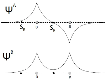
Figure 1: Bonding (ΨB) and anti-bonding (ΨA) wavefunctions of a one-dimensional two site system. The atoms are centered at 0 andRand the radius of the muffin-tin orbital around 0 issR.
The LCAO method and the method of partial waves both have their advantages and disadvantages. The LCAO method transforms the Kohn-Sham equation into an eigenvalue problem, which is not difficult to solve. To give accurate solutions it does, however, need a reasonably complete basis set, which requires many different basisfunctionsχ.
The method of partial waves can give solutions to arbitrary accuracy, but to obtain this solution of set of equations with a non-linear energy dependence needs to be solved.
ψBA =χ(r)±χ(r−R), (14)
where the constantsccan be left out because they are equal by symmetry and can thus be embedded into the basis functionsχ.
This system thus has two possible states. The anti-bonding state ψA, which
corresponds to an energy A, and the bonding stateψB, which corresponds to an energyB.
The bonding and anti-bonding states are shown in Figure 1. Each of these states belongs to one particular energy (A or B) and can thus be described by a single energy-dependent partial wave.
In Figure 1 it can be seen that the anti-bonding wavefunction has a node at the sphere radiussR. At that point the logarithmic derivative in (13) becomes
infinite. The partial wave for this state can thus be found as:
ψA=φ(A, r) (15)
if the logarithmic derivative of A satisfies
D(A) =∞.
Similarly in the bonding state the radial wave-function has zero slope at the sphere radius and the logarithmic derivative is thus zero:
ψB=φ(B, r) (16)
if the logarithmic derivative of B satisfies
D(B) = 0.
To combine the LCAO and the partial wave method, equations (14), (15) and (16) must all be true,and inside the sphere at the origin the orbital centered at
Rmust satisfy
χ(r−R) = [φ(B, r)−φ(A, r)]/2. (17)
Butχ(r−R) is a localized energy independent basis function centered at position
R and we cannot expect it to everywhere match this combination of energy-dependent partial waves. We can expect only that it matches at the boundary of the sphere.
We must thus find a way to satisfy (17). This can be done by choosing the basis functions χ to be the atomic orbitals whose tails are augmented to fit [φ(B, r)−φ(A, r)]/2 inside other spheres.
with respect to energy of the partial waves around some energyEνat the center of our interest.
This method is called thelinear muffin-tin orbitals (LMTO) method because via the Taylor series expansion the relation between partial waves of different energies can be found to linear order as
φ(E, r)≈φ(Eν, r) + (E−Eν) ˙φ(Eν, r),
where we us an overdot to indicate a derivative with respect to energy.
˙
φ(Eν, r)≡∂φ(E, r)
∂E E=E
ν
.
We will from this point on use the notationφ(r) =φ(Eν, r).
Because of this augmentation by the energy derivative the new basis functionsχ
cannot be written as a linear combination of only the partial waves. The energy derivative has to be included as well
χ(r) =X
RL
[φRL(rR)ΠRL+ ˙φRL(rR)ΩRL] +χi(r), (18)
where χi is the component of the basis function in the interstitial region and for notational simplicity theθs are dropped.
To obtain a physical solution, these basis functions and their derivatives need to be continuous. The matrices Π and Ω are coefficient matrices chosen such that the basis functions satisfy this condition.
It is convenient to write (18) in matrix form.
|φiΠ +|φ˙iΩ +|χii=|χi∞, (19)
where|i and|ii denote functions defined in respectively an atomic sphere and
the interstitial region.
3.3
Hamiltonian and Atomic Spheres Approximation
Without loss of generality the partial wavesφ can be chosen to be normalized inside their sphere.
hφRL|φRLi ≡
Z sR
0
φ2R`(E, r)r
2
dr= 1
By differentiating this expression with respect to the energy we see thatφand ˙
φmust be orthogonal.
hφRL|φRL˙ i=
Z sR
0
The partial waves are solutions to the Schr¨odinger equation with the muffin-tin potential inside the spheres.
[−~
2
2m∇
2+V
R(r)]φRL(E,r) =EφRL(E,r). (20)
We are interested in the region around the energy E = Eν. Near this energy
the Schr¨odinger equation can be written in bra-ket notation as
(−~
2
2m∇
2+VR(r)−Eν)|φi= 0,
and by differentiating (20) with respect to energy we obtain
(−~
2
2m∇
2+V
R(r)−Eν)|φ˙i=|φi.
Using these expressions, the orthogonality ofφand ˙φand the expression of the basis functionχin (19), the full Hamiltonian matrix including the contribution of the interstitial region and the non-muffin-tin potential in (10) can be written as
hχ| − ~
2
2m∇
2+V
ks|χi∞= Π∗Ω +hχ| − ~
2
2m∇
2
|χii+hχ|Vnmt|χi∞
=H−EνO,
where the non muffin-tin potentialVnmtis chosen asVksin the interstitial region, and the overlap matrix can be written as
O=hχ|χ|i∞= Π∗Π + Ω∗hφ˙2iΩ +hχ|χii,
wherehφ˙2iis a diagonal matrix with elements
hφ˙2RLi=
Z sR
0 ˙
φ2r`(r)r2dr.
In principle the basis function is known once the matrices Π and Ω are known and the one electron energies can be found. To calculate these matrices one has to integrate over the interstitial region and the non muffin-tin part of the potential. Calculations in the interstitial region can be done with plane waves or muffin-tin orbitals. Plane waves have the disadvantage that a large basis set of 10-50 plane waves is needed to describe the potential in the interstitial region accurately. Muffin-tin orbitals allow us to work with a smaller basis set, but the energies in the interstitial region can, however, not be accurately described with this set.
spheres approximation (ASA), which is actually a combination of two approx-imations. The first approximation is that in the interstitial region the kinetic energy|E−Vi(r)| can be treated as a constant independent of the energy. We will use this approximation later.
The second approximation is that around the atomic sites the potential is spher-ically symmetric, and that these atomic spheres surrounding the atoms can be expanded such that they fill up all of space, with a slight overlap that can be ignored.
The ASA works very well in combination with muffin-tin orbitals, because these orbitals are the solutions to a spherical symmetric potential near the atomic sites. By eliminating the interstitial region in this ASA the muffin-tin orbitals in (19) can be replaced by a new set of basis functions; the so called theta-orbitals, which are orbitals that are augmented in other spheres by only ˙φ func-tions. These orbitals are obtained by multiplying (19) by Π−1 leaving out the interstitial region.
|φi+|φ˙iΩΠ−1=|χi∞Π−1=|Θi∞. (21)
In this set of basis function the Hamiltonian matrix can be represented as
H =hΘ| − ~
2
2m∇
2+Vs|Θi∞= ΩΠ−1+EνO=h+EνO, (22)
where the matrixhis defined as
h=H−EνO= ΩΠ−1, (23)
and the overlap matrix is given by
O=hΘ|Θi∞= 1 +hhφ˙2ih.
The second term of the overlap matrix is second order inhand the real Hamil-tonian can to the second order inhbe approximated by
˜
H =H−Eν.
The only problem remaining now is finding the matrices Ω and Π in the LMTO formalism.
3.4
Logarithmic derivative
In (13) the logarithmic derivative was defined and it was shown that the bond-ing and anti-bondbond-ing wavefunction in a simple two atom system are related to the logarithmic derivative.
waves method, but to ensure continuity of the wavefunction after the augmen-tation, the combination ofφand ˙φ,
Φ(D, r)≡φ(r) +ω(D) ˙φ(r) (24)
should have the same logarithmic derivative as the radial functionφ(r). This is the case if we have:
ω(D) =−φ(sR)
˙
φ(sR)
D−D{φ}
D−D{φ˙},
where we use the notation
D{φ}=sdφ
dr(s)/φ(s),
and
D{φ˙}=sR
dφ˙ dr(sR)/
˙
φ(sR). (25)
The variables Φ and ω are called potential parameters because their values depend intrinsically on the potential. The virtue of a linear method is that these parameters depend on the potential only via the logarithmic derivative.
ω=ω(D), (26)
Φ = Φ(D), (27)
and according to Andersen [5] the Wronskian relation between two different logarithmic derivativesD+ andD− is
(D+−D−)sRΦ+Φ− =ω−−ω+, (28)
whereω+ andω− areω(D) for respectivelyD+ andD−.
3.5
Structure Constants
Muffin-tin orbitals are the solutions of a spherically symmetric potential in spheres surrounding the atomic-sites and are thus angular-momentum eigen-functions, which can be separated into a radial part and an angular part.
χRL(r) =χR`(r)YL(ˆr).
In the interstitial region the tail function χi
RL(r) is a solution to (7) for a
constant potential i.e. to the Helmholtz equation.
whereκ2=E−V is a constant. Because the packing of the atomic spheres in metal is very close, especially in the ASA,κ2 is very small and for simplicity we make the choiceE=V, such thatκ2= 0.
In this case (29) reduces to the Laplace equation whose solutions are propor-tional tor−`−1 andr`.
The radial part of the tail function extends throughout the whole crystal and must thus be chosen such that it vanishes as r goes to infinity.
χiR`(rR) = rR
s !−`−1
,
wheresis a scaling constant, which can be chosen arbitrarily.
In the LMTO method the tail function is augmented in all spheres. It can thus be expanded around the other sites using the multipole expansion1.
rR s
!−`−1
YL(ˆrR) =−
X
L0 rR0
s !`0
YL0(ˆrR0)
2(2`0+ 1)SR0L0,RL (30)
where the coefficients S are called the structure constants, which are given by
SR0`0m0,R`m= (4π)
1
2g`0m0,`m
R−R0
s
!−`0−`−1
Y`?0−`,m0−m(R ˆ−R0), (31)
with
g`0m0,`m = (−1)`+m+1 2
"
(2`0+ 1)(2`+ 1)(`0+`+m0−m)!(`0+`−m0+m)! (2`0+ 2`+ 1)(`0+m0)!(`0−m0)!(`+m)!(`−m)!
#12
.
The head and tail of the LMTO must match continuously on the sphere radius
sRand we can thus define the LMTO as
χRL(r) =YL(ˆr)
Φ−R`(−`−1, r) forr≤sR
(Sr
R)
−`−1Φ−
R`(, `−1, sR) forr≥sR
, (32)
where Φ−R` is given by (24), where the logarithmic derivative is D = −`−1, which is the logarithmic derivative ofr−`−1.
Using (30) and (32) the contribution of an orbital at positionRinside a sphere at positionR0 can be seen to be
χRL(rR) =−
X
L0
Φ+R0L0(rR0 )
2(2`0+ 1)φ+
R0`0(s0R) sR0
s `0
SR0L0,RL
s
sR
−`−1
Φ−R`(sR),
(33)
where Φ+R` is given by (24) for the logarithmic derivative D =`, which is the logarithmic derivative ofr`.
3.6
Π
and
Ω
matrices
Equation (33) can be simplified by introducing two new parameters.
√
∆≡ s
sR
−`−1s
2
12
Φ−(−`−1, sR),
√
Γ≡2(2`+ 1) s
sR
`s
2
12
Φ+(`, sR)≡Q∆
1 2,
where Q is called thescreening parameter.
Using these parameters the relation from (28) can be rewritten as
√
∆√Γ = (2`+ 1)sRΦ−(−`−1, sR)Φ+(`, sR) =ω−−ω+, (34)
whereω+ andω− areω(D) for respectivelyD=`andD=`−1.
Using the potential parameters, (33) can be written as
χRL(rR) =−
X
L0
Φ+R0L0(rR0 )Γ
−1/2
R0L0SR0L0,RL∆1RL/2. (35)
Equation (32) gives the shape of the LMTO inside its own sphere and (35) gives the contribution to the LMTO inside this sphere from the LMTOs centered at other sides. Taking into account all these contributions, the complete basis functions can be written in matrix notation as
|Φ−i − |Φ+iΓ−12S∆12 +|χii=|χi∞. (36)
According to (24) the functions Φ+ and Φ− are given by
|Φ+i=|φi+ω+|φ˙i,
|φ−i=|φi+ω−|φ˙i,
and the expressions for the Π and Ω matrix are then given by
Π = 1−Γ−12S∆ 1
2 (37)
and
Ω =ω−−ω+Γ−
1 2S∆
1
3.7
LMTO-ASA Hamiltonian
Using the atomic sphere approximation (ASA), the interstitial region is elimi-nated and the Hamiltonian can be written as in (22). The matrices Π−1 and Ω in the Hamiltonian can be obtained from (37) and (38) as
Π−1= ∆−12(Q−S)−1Γ 1 2,
and
Ω = (ω−+ω+) +ω+Γ−
1
2(Q−S)∆12,
whereQis now used as a diagonal matrix with the valuesQRL on its diagonal.
Using these relations and (34) and (22) we obtain an expression forh= ΩΠ−1.
h= Γ12(Q−S)−1Γ
1 2 +ω+
= ∆12S(1−Q−1S)−1∆1/2+ω−.
The full Hamiltonian can then be obtained as
˜
HRL,R0L0 = ∆
1 2
R`SRL,R˜ 0L0∆
1 2
R0`0+ω−+EνR` (39)
= ∆ 1 2
R`SRL,R˜ 0L0∆
1 2
R0`0+CR`δRR0δLL0, (40)
where the ˜S denote thescreened structure constants.
˜
S=S(1−Q−1S)−1.
This is the reason why we call Q, the screening parameter, because it relates the ordinary structure constantsS to the screened structure constants ˜S.
3.8
Canonical Bands
We start by discussing the case without screening, which is obtained by setting the screening matrixQ−1= 0. The screened structure constants then reduce to the ordinary structure constants and the Hamiltonian can be written as
H=C+√∆S√∆.
Our goal is the find the so-called energy bandsε(k), which describe the energies that electrons can have.
To calculate these energy bands one needs to transform the Hamiltonian from real space into the so-calledk-space, which is essentially the Fourier transform of the real lattice. The Hamiltonian is transformed from real space to k-space by performing a Bloch summation over all the atoms in the lattice.
H`m,`k 0m0 = X
R6=0
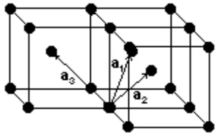
As taking a summation over an infinite lattice is not possible, the Bloch summa-tion must be performed only over all neighbours within a certain radius. This can be done by setting up the 3 spanning vectors such that the lattice can be generated by a linear combination of these vectors. We will do a sample calcu-lation for vanadium, which has a bcc (body centered cubic) lattice, which is a cubic lattice with lattice points on all its vertices and one in the center of the cube. Another useful lattice is the fcc (face centered cubic) lattice, which is a cubic lattice with lattice points on all its vertices an on the center of its faces. A bcc lattice is shown in Figure (2). The corresponding lattice vectors are
a1=
a
2
1 1
−1
, a2=
a
2
1
−1 1
, a3=
a
2
−1 1 1
,
[image:17.612.197.413.319.451.2]where a is the lattice constant, which is the length of one edge of the cubic lattice.
Figure 2: bcc lattice spanned by the vectorsa1,a2 anda3.
A lattice of neighbours is then a set containing the linear combinations of these lattice vectors.
RN ={n1a1+n2a2+n3a3 |n1, n2, n3∈ {−N, N}}
We will callRN the set containing N shells of neighbours.
To each lattice in real space belongs areciprocal lattice in k-space, spanned by the vectorsb1, b2 andb3, which are defined as
b1= 2π
a2×a3
a1·(a2×a3)
b2= 2π
a3×a1
a2·(a3×a1)
b3= 2π
a1×a2
a3·(a1×a2)
As the scaling matrices ∆ and Γ are independent of the shape of the lattice, the Bloch summation can be done using only the structure constants.
S`m,`k 0m0 = X
R∈RN
eik·RS0L,RL0.
The so-calledcanonical bandscan be obtained by neglectinghybridization, which is the influence the different bands have on each other. This can be done by separately diagonalizing the diagonal blocks`=`0 of the matrixSk
`m,`0m0.
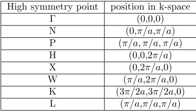
Energy bands are drawn between so called high symmetry points, which are points in k-space that represent the symmetry of the lattice. Some high sym-metry points are listed in table 1.
The bcc canonicald-bands (`= 2) are shown in Figure 4.
High symmetry point position in k-space
Γ (0,0,0)
N (0,π/a,π/a)
P (π/a, π/a, π/a)
H (0,0,2π/a)
X (0,2π/a,0)
W (π/a,2π/a,0)
[image:18.612.205.405.300.413.2]K (3π/2a,3π/2a,0) L (π/a,π/a,π/a)
Figure 3: Some high symmetry points for an fcc lattice ink-space.
-15 -10 -5 0 5 10 15
Γ N
Figure 4: Canonicald-bands for a bcc lattice calculated with 20 shells of neigh-bours. The bands are dimensionless and are shown between the two high sym-metry points Γ andN. These canonical bands give a first order approximation of the real energy of bcc materials.
[image:19.612.182.430.389.570.2]correspond electron energy. Because the structure constants are dimensionless quantities, the canonical bands are also dimensionless. Their dimensionless values are those for the structure constants in (31) when sis chose as the so-called Wigner-Seitz radius.
s=a 3
8π 13
The convergence of the canonical bands can be made a bit more concrete by looking at the behaviour of one of the bands at the point Γ for a different number of shells of neighbours, as shown in Table 2. It can be seen from the last column of the table that the effect of taking into account more neighboring shells becomes weaker very quickly. The canonical bands obtained will thus quickly converge.
Neighbour shells Energy at Γ Contribution of new shells
1 -3.852 -3.852
2 -3.685 0.168
4 -3.623 0.062
8 -3.603 0.020
16 -3.598 0.005
[image:20.612.167.446.302.391.2]32 -3.596 0.002
Table 2: Energy of the lowest bcc canonical bands at the high symmetry point Γ computed with various numbers of shells of neighbours.
3.9
Hybridized Bands
The canonical bands are very similar to real energy bands. They form a dimen-sionless template for the real energy bands, but to obtain the real bands three additional steps have to be made.
Firstly the structure constants have to be screened by the screening parameter
Q.
Because both the structure constants and the screening parameter are dimen-sionless, the bands have to be scaled and positioned at the right energy for a specific system, which is done by the parameters ∆ (or Γ) andC respectively.
All of these steps are incorporated in the Hamiltonian in (40). The correspond-ing Hamiltonian ink-space is given by (41) by replacingH with ˜H.
of these bands depends on the potential parameters, such asEν,ω−, Φ−and Φ+.
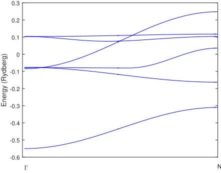
These parameters are all material dependent and can be found in literature [5]. In Figure 5 the hybridized energy bands for bcc-vanadium are shown.
-0.6 -0.5 -0.4 -0.3 -0.2 -0.1 0 0.1 0.2 0.3
Energy (Rydberg)
[image:21.612.190.411.183.356.2]Γ N
Figure 5: Hybridized energy bands for bcc vanadium calculated with two shells of nearest neighbours.
The Hybridized energy bands are real energy bands, meaning that each line represents a dispersion relationε(k) for an electron. All the possible energies an electron can have, can be found in such a band diagram.
The numerical convergence of the LMTO method is very good. From Table 3 it can be seen that the influence of adding a second shell of nearest neighbours on the energies is already very small and that further shells will contribute very little.
N = 1 N = 2
-0.5678 -0.5757 -0.0804 -0.0824 -0.0770 -0.0816 -0.0736 -0.0808 0.1054 0.1099 0.1055 0.1099
Table 3: Energies of the hybridized vanadium bands in Rydberg at the point Γ for a different number of neighboring shells.
the band structures of vanadium, copper and cobalt respectively. These band structures were calculated using the LMTO code.
−1 −0.8 −0.6 −0.4 −0.2 0 0.2 0.4 0.6
Γ N P Γ H N
Energy (Rydberg)
[image:23.612.137.467.132.311.2]Vanadium
Figure 6: Vanadium energy bands.
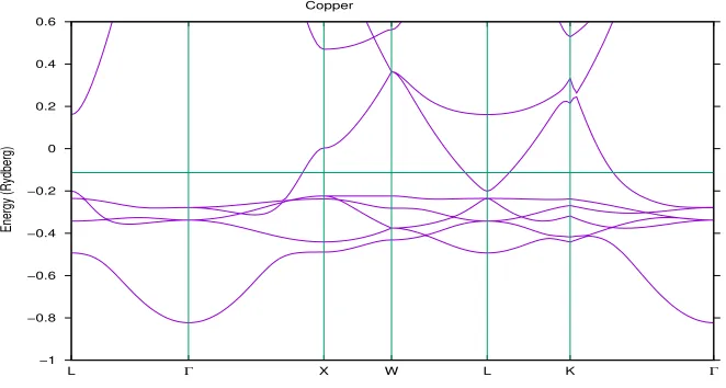
−1 −0.8 −0.6 −0.4 −0.2 0 0.2 0.4 0.6
L Γ X W L K Γ
Energy (Rydberg)
Copper
[image:23.612.137.468.356.533.2]−1 −0.8 −0.6 −0.4 −0.2 0 0.2 0.4 0.6
L Γ X W L K Γ
Energy (Rydberg)
Cobalt majority spin
(a)
−1 −0.8 −0.6 −0.4 −0.2 0 0.2 0.4 0.6
L Γ X W L K Γ
Energy (Rydberg)
Cobalt minority spin
[image:24.612.136.466.131.519.2](b)
4
Transport
[image:25.612.174.441.185.292.2]4.1
Scattering Formalism
Figure 9: Schematic of the configuration used for transport calculations. A scattering region S is sandwiched by left (L) and right (R) leads. The scattering region is divided intoN layers.
One of the applications of muffin-tin orbitals is the calculation of the conduc-tance of metallic interfaces, such as the one depicted in Figure 9. Such an interface can be divided into three regions: The left and right leads, which are assumed to be ideal and periodic conductors,such that the Bloch theorem can be used, and the scattering region,which is the region sandwiched between these two ideal leads.
In electronic transport the concept of a scattering matrix is very important. Scattering matrices are used to relate incoming and outcome waves trough a barrier.
F G
=
t γ
γ∗ t∗
A B
,
whereAand B are the amplitudes of respectively the right-going and the left-going waves in the left lead, and F and G are the amplitudes of respectively the right and left-going waves in the right lead. In the scattering matrix the coefficienttis the probability that a right going wave on the left is transmitted to a right going wave on the right.
Conductance through an interface can be described in terms of scattering ma-trices by the Landauer-B¨utticker formula.
G= e
2
h X
n,m
|tn,m|2, (42)
wheretn,mis the probability that a statenin the left lead scatters into a state
For this purpose we are concerned with only a single energy and it is desirable not to expand the wavefunctionψ(r) in a basis of linear muffin-tin orbitals, but to expend it into energy dependent orbitals. We define the radial part of these orbitals as
χR`(E, r) =
φ(E, r)−DR`(E)+`+1
2`+1
r sR
`
φR`(E, sR) forr≤sR
`−DR`(E)
2`+1
r sR
−`−1
φR`(E, sR) forr≥sR.
Defined this way the MTO is continuous and differentiable everywhere, and is thus a physical basis function. The notation can be cleaned up by introducing two new quantities.
|r+i ≡
rR
sR
` YL(ˆrR)
2(2`+ 1),
and
P(E)≡2(2`+ 1)D(E) +`+ 1
D(E)−` , (43)
whereP(E) is called thepotential function.
We can still use (30) to expand the tails of the orbitals. The total orbital can thus be written in matrix form as
|φ(E)i+|r+iP(E)−Sχ(E, sR) =|χ(E)i∞.
The wavefunction can be found as a linear combination of these MTO’s centered at different sites.
Ψ(E,r) =X
RL
χ(E,rR)CRL. (44)
The wavefunction can thus be represented by the expansion coefficients.
Ψ= .. .
ci−1
ci ci+1
.. . .
From the partial wave point of view we already know thatφ(E, r)YL(ˆr) is a
X
R0L0 h
PRL(E)δRR0δLL0 −SRL,R0L0
i
CR0L0 = 0.
This is called thetail cancellation equation.
For performing calculations it is impractical that the MTO’s have an infinite range. This can be solved in a simple way by introducing screening constants
αR` such that the tail-cancellation equation changes to
X
R0L0 h
PRLα (E)δRR0δLL0 −SRL,Rα 0L0 i
CRα0L0 = 0, (45)
Where the screened potential function matrix and the screened structure con-stants are given by [6]
P`α(E) =P`(E)
h
1−αP`(E)i
−1
,
SRL,Rα 0L0 =SRL,R0L0 h
1−αSRL,R0L0 i−1
.
Due to this screening the structure constants can have a very short range. The set of screening constants for which the range of the structure constants is minimized is denoted byβR`.
We will take into account only the interaction between neighbouring layers. The structure constant matrix can then be written as
S=
. .. . . . 0 0 0
..
. Si−1,i−1 Si−1,i 0 0
0 Si−1,i Si,i Si+1,i 0
0 0 Si,i+1 Si+1,i+1 ...
0 0 0 . . . . ..
, (46)
Where the structure matrixSi,jdenotes the structure interactions between sites
in layeriandj.
Using (46) we can write out the tail cancellation equation in its terms to obtain the so-calledequation of motion.
−Sβi,i−1Ci−1+
Pβi,i(E)−Sβi,iCi−S β
i,i+1Ci+1= 0, (47)
where Ci is an M dimensional vector, where M = (`max+ 1)2N, N is the
4.2
Leads
In a periodic potential, such as in an ideal metal, the wavefunction should satisfy Bloch’s theorem and the expansion coefficientsCshould be related by
Cn =λCn−1, (48)
whereλis the Bloch phase factor.
λ=eik·T,
withTthe vector connecting two equivalent sites in neighbouring layers.
Using (48) the equation of motion can be written in matrix form.
S−i,i1+1(Pi,i−Si,i) S−i,i1+1Si,i−1
1 0
Ci
Ci−1
=λ
Ci
Ci−1
This eigenvalue problem has 2M eigenvalues and eigenvectors. The eigenvectors are divided intoM right-going waves andM left-going waves.
Following the notation introduced by Ando [1], let u1(−), . . . ,uM(−) be the
vectorsC0 of the left-going solutions corresponding to the eigenvalues
λ1(−), . . . , λM(−) andu1(+), . . . ,uM(+) the vectors C0 of the right-going
so-lutions corresponding to the eigenvaluesλ1(+), . . . , λM(+).
We then defineU(±) and Λ(±) as the matrices
U(±) =(u1(±). . .uM(±)),
and
Λ(±) =
λ1(±)
. ..
λM(±)
.
Any solution to the equation of motion at in the layerC0 can be written as a linear combination of left or right going solutions.
C0(±) =U(±)C(±),
whereC(±) is a vector of expansion coefficients.
By (48) in general any solution can be written as
Two solutions can be related as
Cj(±) =F(±)j−j 0
C0j(±), (49)
with
F(±) =U(±)Λ(±)U−1(±).
4.3
Scattering region
Now that the relation between two solutions is known, it can be applied to a scattering problem. We consider the scattering problem shown in Figure 9: a scattering region consisting of N layers, which has an ideal lead attached to both its left and right side.
By linearity of the wave equation the total amplitude of the wave at each cell can be written as the sum the right-going and the left-going waves at that point.
Cj =Cj(+) +Cj(−).
We consider the case where a current is sent into the left lead. At the left end of the scattering region there are left-going and right-going solutions resulting from reflection and transmission. Using (49) the amplitude at cell -1 inside the left lead can then be related to the amplitude at cell 0.
C−1=F−1(−)C0+ [F−1(+)−F−1(−)]C0(+).
The equation of motion at cell 0 can then be written as
−Sβ0,−1C−1= (P
β
0,0−S
β
0,0)C0−S
β
0,1C1= 0,
which becomes:
(P0,0−˜S0,0)C0−S0,1C1=S0,−1[F−1(+)−F−1(−)]C0(+),
with
˜
S0,0=S0,0+F−1(−). (50)
This expression shows the basis principle of thewave function matching method. By matching the waves coming from the left lead with the waves in the scattering region, the wave amplitude in all layers in the left lead can be written in terms of the amplitudeC0and the whole left lead essentially turns into a single layer
C0.
To the right of the scattering region there are only right-going waves, because the right lead,as an ideal conductor, does not reflect. Amplitudes of successive layers in this lead can thus written in terms of the previous layer.
The equation of motion in layerN+ 1 can then be written as
(PN+1,N+1−S˜N+1,N+1)CN+1−SN+1,NCN = 0. (51)
Equations (50) and (51) can be seen as boundary conditions on the scattering region, and the problem of finding the conductance through the interface is reduced from a problem over an infinite region to a problem over only the scattering region.
For the whole scattering region the tail cancellation matrix can be written as
P−S˜=
(P−S˜)0,0 −S0,1 0 . . . 0 0
−S1,0 (P−S)1,1 −S1,2 . . . 0 0
0 −S2,1 (P−S)2,2 . . . 0 0
..
. ... ... . .. ... 0
0 0 . . . (P−S)N,N −SN,N+1
0 0 0 . . . −SN+1,N+1 (P−S˜)N+1,N+1
.
The scattering problem can then written as a set of in-homogeneous linear equations.
(P−˜S)
C0 C1 C2 .. . CN
CN+1
=
S0,−1[F−1(+)−F−1(−)]C0(+)
0 0 .. . 0 0 .
The solution to which is given by
C0 C1 C2 .. . CN
CN+1
=g
S0,−1[F−1(+)−F−1(−)]C0(+)
0 0 .. . 0 0 ,
wheregis defined as
g= (P−˜S)−1.
The amplitude of the wave at the right of the scattering regionCN+1 can now be related to the incoming wave amplitudeC0.
From this expression the transmission coefficienttµν for a incident waveν with velocityυν and outgoing waveµwith velocity υµ can be expressed as
tµν =
υµ
υν 1/2
{U−1(+)gN+1,0S0,−1[F−1(+)−F−1(−)]U(+)}µν (53)
Now the conductance of the interface can be calculated using the Landauer-Buttiker equation (42).
[image:31.612.258.352.287.393.2]4.4
Cu-Co interface
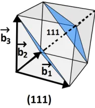
Figure 10: Cubic crystal with (111) planes shown in blue. These planes are perpendicular to the vector 1b1+ 1b2+ 1b3indicated by the broken line.
We are now ready to commit ourselves to finding the conductance through a copper-cobalt interface.
The wavefunction matching method explain previously can be used for this sit-uation. We are interested in transport across the (111) plan, which is the plane in a cubic crystal perpendicular to the reciprocal lattice vector 1b1+ 1b2+ 1b3,
as shown in Figure (10). We use the transport code developed by the chair of Computational Materials Science, in which the scattering formalism is combined with the wavefunction matching method. With this code the transmission coef-ficients in (53) can be calculated as a function of the Bloch-wave vector parallel to the (111) directionk||.
All the different Bloch statesk|| can be visualized by a projection of the Fermi
(a) (b)
[image:32.612.153.465.120.374.2](c) (d)
Figure 11: Top row: projection of the Fermi surfaces of copper (a) and cobalt (b) onto the (111) plane, perpendicular to the transport direction. Bottom row: Transmission probability as a function ofk||,T(k||) of an ordered copper-cobalt interface for majority spin (c) and minority spin(a). The transmission probabil-ity is indicated by the color scheme, with red being complete transmission and blue being total reflection. White indicates points where there is no state.
These Fermi surface projections already give a good estimate of the Transmis-sion probability spectrum for the interface. In ordered interfaces, which we are dealing with now, the crystal momentum parallel to the interfacek|| must be
conserved. There can only be transmission for a givenk||if their exists a state
for it in both copper and cobalt. If there exists a state in copper, but there is no corresponding state in cobalt there will be no transmission and the electron will be totally reflected.
The transmission spectrum for the majority-spin states as shown in Figure 11c follows this intuitive picture quite nicely. It can be seen that if there is no state
k|| in either copper or cobalt there is no transmission and for other states the
transmission is almost everywhere unity.
The transmission spectrum for the minority-spin states, shown in Figure 11d is more complicated. The transmission is not uniform for thek|| points which
above the Fermi energy, which is the energy of the highest occupied, and are thus only partially occupied.These band can thus all contribute a statek|| for
transmission. This means that an propagating state in copper with momentum
k|| is transmitted into a combination of the propagating states in cobalt with
the samek||.
This however still does not fully explain the minority transmission probabilities. Fur a full explanation the k-points need to be examined one by one. At each point there are different propagating states in copper and cobalt, with odd or even symmetry. Propagating from an even to an odd state and vice versa is not allowed, and at some points this results in vanishing transmission probabilities, while in other points these can become very large.
By comparing the transmission probabilities for the majority and minority spin cases, it can be seen that the total transmission of majority spin electrons is higher than that of the minority spin electrons, by about 20%. In this way ferromagnetic materials like cobalt thus act as a spin-polarizer, allowing more majority spin electrons than minority electrons. Such a polarizer is very useful in the field ofspintronics (spin electronics), which has many applications, such as hard drives or spin-bases transistors.
5
Summary
&
Conclusion
In this paper we calculated the energy bands of vanadium, copper and cobalt, and the transmission probability spectrum through a copper-cobalt interface using scattering formalism and wavefunction matching, where the electronic structure was calculated using the LMTO-ASA formalism within the framework of density functional theory.
In particular, we explained how in DFT a 3N-dimensional quantum mechanical problem is transformed to a 3-dimensional problem, making numerical solutions possible, and how this framework can be implemented using the Schr¨odinger-like Kohn-Sham equations to obtain solutions for metallic structures.
Furthermore, we explained the method of muffin-tin orbitals and showed that these orbitals form a flexible basis set for solving the Kohn-Sham equations. For energy intervals we showed that these orbitals can be modified to linear muffin-tin orbitals using tail augmentation and can be used to calculate band structures of metals.
We demonstrated that for a single energy the muffin-tin orbitals can be used in combination with the tail cancellation condition to give equations for a scatter-ing problem which can be solved with wavefunction matchscatter-ing to obtain trans-mission probabilities and subsequently the conductivity of an interface.
plane. Lastly we explained how the magnetic properties of cobalt lead to differ-ent transmission spectra for majority and minority spin electrons.
Furthermore we have only looked at ordered interfaces with equal lattice pa-rameters in all layers of the scattering region. Real interfaces often have some form of disorder and the lead can have very different lattice parameters. An approach that could be able to take into account disorder and different lattice parameters is by extending the current wave function matching model by the use ofsupercells [6].
References
[1] T. Ando, “Quantum point contacts in magnetic fields,”Phys. Rev. B, 1991.
[2] G. Brockset al., “Calculating scattering matrices by wave function match-ing,” Ψk newsletter, 2007.
[3] P. Hohenberg and W. Kohn, “Inhomogeneous electron gas,”Phys. Rev. B, 1964.
[4] W. Kohn and L. J. Sham, “Self-consistent equations including exchange and correlation effects,”Phys. Rev. B, 1964.
[5] O. K. Andersen, “Linear methods in band theory,”Phy. Rev. B, 1975.
[6] K. Xiaet al., “First-principles scattering matrices for spin transport,”Phys.